1. Introduction
Gusts have attracted significant interest in aeronautical applications over the last decade (Jones & Cetiner Reference Jones and Cetiner2021). They are being studied for the development of urban mobility and aircraft safety, for example.
The literature (Jones & Cetiner Reference Jones and Cetiner2021; Jones, Cetiner & Smith Reference Jones, Cetiner and Smith2022) proposes to classify gusts into three categories: (i) streamwise gusts, (ii) transverse gusts, and (iii) vortex gusts. Streamwise gusts are disturbances parallel to the flow, transverse gusts are disturbances perpendicular to the flow, and vortex gusts are bi-directional disturbances originating from a vortex singularity of circulation
 $\varGamma _g$
. In practice, vortex gusts can occur in a variety of situations, such as downstream of buildings or aircraft. In all cases, the instantaneous change in freestream velocity due to the gust induces a straightforward change in instantaneous aerodynamic loads due to their dependency on the freestream velocity squared. It is therefore usually convenient, when possible, to define instantaneous aerodynamic coefficients as instantaneous forces and moments normalised by the instantaneous freestream velocity squared. In addition to this trivial effect, gusts may induce changes in instantaneous aerodynamic coefficients.
In the case of streamwise gusts, changes in instantaneous aerodynamic coefficients are due to changes in instantaneous Reynolds number. The latter have negligible effects at high Reynolds numbers where the boundary layer over a wing is turbulent, but may strongly affect flow topology at moderate Reynolds numbers where the laminar boundary layer typically undergoes laminar separation, transition and reattachment. In such cases, it was shown that the sensitivity of the resulting laminar separation bubble to freestream Reynolds number results in high sensitivity of instantaneous aerodynamic coefficients to streamwise gusts (Jardin, Ferrand & Gowree Reference Jardin, Ferrand and Gowree2025).
The effect of transverse gusts on instantaneous aerodynamic coefficients is relatively straightforward in that the additional freestream transverse velocity component leads to a change in the effective angle of attack of the wing (Helmbold Reference Helmbold1942; Biler et al. Reference Biler, Sedky, Jones, Saritas and Cetiner2021; Jones et al. Reference Jones, Cetiner and Smith2022). For example, in a linear framework, the change in effective angle of attack induced by transverse velocity component
 $V_g$
is
 $V_g/U_{\infty }$
(where
 $U_{\infty }$
is the freestream velocity in the absence of gusts), and the corresponding lift increment is
 $2\pi V_g/U_{\infty }$
. Yet the response in instantaneous lift coefficient to transverse gust is not always linear. For example, Corkery, Babinsky & Harvey (Reference Corkery, Babinsky and Harvey2018) showed that a large-amplitude transverse gust induces the formation of a leading-edge vortex (LEV), which is associated with strong lift generation.
In the case of vortex gusts, changes in both instantaneous Reynolds number and angle of attack come into play. Moreover, there is a strong coupling between the dynamics of the vortex gust and the wing. That is, in addition to being modified by the potential flow around the wing, the circulation and trajectory of the vortex gust are modified by its interaction with the wing boundary layer, resulting in local flow separation and complex vorticity dynamics. An example of airfoil–vortex gust interaction is provided by Biler et al. (Reference Biler, Sedky, Jones, Saritas and Cetiner2021), where it is shown that the vortex-induced velocity field is significantly affected by the presence of the airfoil, and that the airfoil boundary layer is significantly affected by the vortex gust.
The complex physics behind wing–vortex gust interaction requires a specific mitigation strategy. That is, the control strategy must account for complex flow phenomena such as LEV formation and generation of secondary vorticity. Gust mitigation strategies presented in the literature can be grouped into two categories: strategies based on low-order models, and model-free strategies. The former have the advantage of directly incorporating physics into the derivation of the controller, but can be limited by the model’s assumptions. Conversely, the latter approach benefits from not relying on any explicit physical models. However, it then sacrifices its ability to incorporate prior physical knowledge. An example of gust mitigation control based on a low-order model is provided by Andreu-Angulo & Babinsky (Reference Andreu-Angulo and Babinsky2020) and Sedky et al. (Reference Sedky, Gementzopoulos, Andreu-Angulo, Lagor and Jones2022). In their work, the authors sought a pitch motion that induces the lift modelled by Wagner (Reference Wagner1925) to counterbalance that induced by the gust as modelled by Küssner (Reference Küssner1932). Conversely, Kazarin et al. (Reference Kazarin, Golubev, MacKunis and Moreno2021) and Herrmann et al. (Reference Herrmann, Brunton, Pohl and Semaan2022) provide examples of model-free approaches, where the actuation strategy relies on online flow data instead of an aerodynamic model. It should be emphasised that each of these works builds its control functions either on a simplified aerodynamic model or on control function simplifications. For instance, Andreu-Angulo & Babinsky (Reference Andreu-Angulo and Babinsky2020) model the gust according to potential flow assumptions, while Sedky et al. (Reference Sedky, Gementzopoulos, Andreu-Angulo, Lagor and Jones2022) and Herrmann et al. (Reference Herrmann, Brunton, Pohl and Semaan2022) consider linear control functions, and finally Kazarin et al. (Reference Kazarin, Golubev, MacKunis and Moreno2021) bypasses the unsteady aerodynamic model by treating the gust as an unknown lift disturbance.
Data-driven methods have expanded the range of tools available for gust-related tasks, particularly in the areas of reduced-order modelling, sensing and control. Fukami & Taira (Reference Fukami and Taira2023) and Smith et al. (Reference Smith, Fukami, Sedky, Jones and Taira2024) use the nonlinearity of neural networks to learn a low-dimensional representation of high-dimensional gust-induced flows. Mousavi & Eldredge (Reference Mousavi and Eldredge2025) and Zhong et al. (Reference Zhong2023) use machine learning to reconstruct vortex-induced flows from sparse sensor measurements. In terms of control issues, Fukami, Nakao & Taira (Reference Fukami, Nakao and Taira2024) propose a gust mitigation technique that aims to reduce the gust-induced lift perturbation through phase-amplitude modulation of a low-dimensional flow state representation.
This work contributes to ongoing efforts on gust control using machine learning techniques. Our aim is to mitigate the lift induced by vortex gusts by deriving an airfoil pitch controller without simplifying the model or control function. Particular attention is paid to the interaction between the airfoil and the vortex. To this end, we build the controller as an artificial neural network (ANN), with its parameters being determined using deep reinforcement learning (DRL) based on states provided by direct numerical resolution of the Navier–Stokes equations. Precisely, at each discrete interaction step of duration
 ${\rm d}t_c$
, the ANN controller observes the system state
 $s_t$
produced by the unsteady flow solver. The ANN then outputs a new pitch rate
 $\dot {\alpha }_t$
, which is applied to the airfoil for the next iterations of the flow solver, triggering the transition from the previous state
 $s_t$
to
 $s_{t+{\rm d}t_c}$
. Finally, the ANN controller receives a reward
 $r_t$
computed from
 $s_{t+{\rm d}t_c}$
. Based on a set of samples
 $\{(s_t, \dot {\alpha }_t, r_t, s_{t+{\rm d}t_c})\}$
, the DRL algorithm optimises the ANN parameters so that the state-control sequence
 $(s_0, \dot {\alpha }_0, \ldots, s_t, \dot {\alpha }_t, \ldots, s_{T_f}, \dot {\alpha }_{T_f})$
maximises the criterion
 $J = \sum _{t=0}^{T_f} r_t$
, where
 $T_f$
is the final simulation time.
In recent years, DRL has been applied to a variety of fluid control problems. Researchers have recently used DRL to learn effortless swimming strategies (Novati et al. Reference Novati, Verma, Alexeev, Rossinelli, van Rees, Wim and Koumoutsakos2017; Verma, Novati & Koumoutsakos Reference Verma, Novati and Koumoutsakos2018; Gunnarson et al. Reference Gunnarson, Mandralis, Novati, Koumoutsakos and Dabiri2021), reduce drag around a cylinder and in turbulent channel flows (Rabault et al. Reference Rabault, Kuchta, Jensen, Réglade and Cerardi2019; Paris, Beneddine & Dandois Reference Paris, Beneddine and Dandois2021; Ren, Rabault & Tang Reference Ren, Rabault and Tang2021; Guastoni et al. Reference Guastoni, Rabault, Schlatter, Azizpour and Vinuesa2023; Sonoda et al. Reference Sonoda, Liu, Itoh and Hasegawa2023), control Rayleigh–Bénard convection (Beintema et al. Reference Beintema, Corbetta, Biferale and Toschi2020; Vignon et al. Reference Vignon, Rabault, Vasanth, Alcántara-Ávila, Mortensen and Vinuesa2023), and model turbulence (Beck & Kurz Reference Beck and Kurz2021; Kurz, Offenhäuser & Beck Reference Kurz, Offenhäuser and Beck2023). Nevertheless, learning control strategies from Navier–Stokes equations using DRL raises two main issues: (i) the choice of the input state fed to the controller, and (ii) the computational cost of the DRL computational fluid dynamics strategy.
The question of computational cost is not critical in our case due to the relatively low Reynolds number considered, which allows numerical resolution of the Navier–Stokes equations in a reasonable amount of time. For higher Reynolds number cases where computational cost becomes prohibitive, an appealing approach is transfer learning, where high-fidelity flow solver is only used to evaluate or refine a network previously trained on reduced-order models (Liu, Beckers & Eldredge Reference Liu, Beckers and Eldredge2025; Usandivaras et al. Reference Usandivaras, Bauerheim, Cuenot and Urbano2025). Another approach relies on the parallelisation of the DRL algorithm, referred to as the ‘multi-environment approach’ by Rabault & Kuhnle (Reference Rabault and Kuhnle2019).
Regarding point (i), the input state
 $s_t$
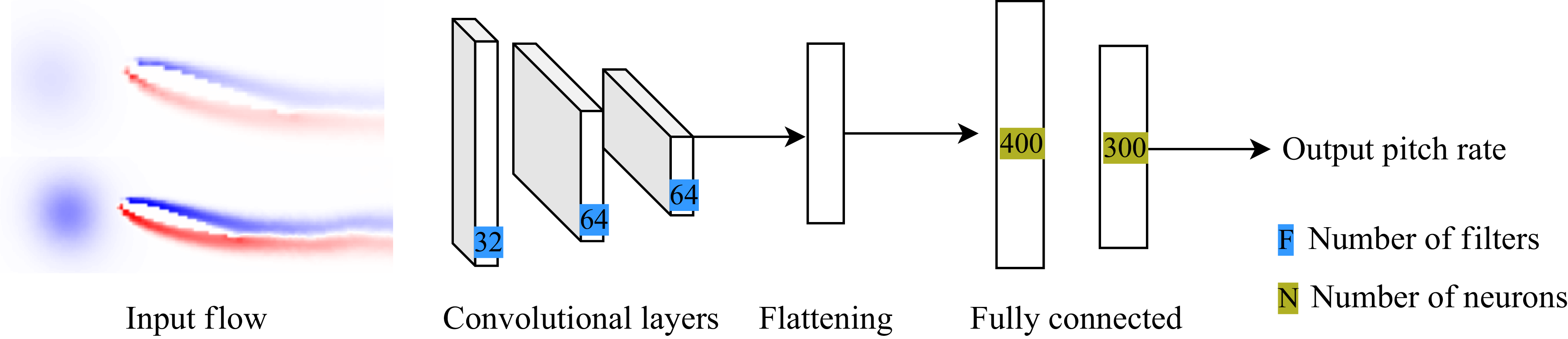
should ideally be the entire velocity field, but simple multi-layer perceptrons cannot process efficiently such large inputs. Rabault et al. (Reference Rabault, Kuchta, Jensen, Réglade and Cerardi2019) address this issue by using a small set of velocity and pressure probes; however, this is suboptimal (Paris et al. Reference Paris, Beneddine and Dandois2021). Therefore, we circumvent this problem by adding convolutional layers to our controller to process the entire system state.
The application of DRL to aerodynamic disturbance mitigation has been recently addressed by Renn & Gharib (Reference Renn and Gharib2022), Beckers & Eldredge (Reference Beckers and Eldredge2024), Martin et al. (Reference Martin, Jardin, Rachelson and Bauerheim2024) and Liu & Eldredge (Reference Liu and Eldredge2025). Each of these works investigates how to learn mitigation strategies when the full flow state is unknown and only onboard measurements are available, albeit using different approaches. Beckers & Eldredge (Reference Beckers and Eldredge2024) explore which data from onboard sensors should or should not be included in the controller’s inputs. Martin et al. (Reference Martin, Jardin, Rachelson and Bauerheim2024) focus on estimating the unknown states using a Kalman filter, whereas Renn & Gharib (Reference Renn and Gharib2022) and Liu & Eldredge (Reference Liu and Eldredge2025) respectively employ a recurrent neural network and a transformer to learn a representation of these unknown states. These studies also differ in terms of model fidelity. Martin et al. (Reference Martin, Jardin, Rachelson and Bauerheim2024) have used an unsteady vortex lattice method assuming an infinite Reynolds number, Beckers & Eldredge (Reference Beckers and Eldredge2024) and Liu & Eldredge (Reference Liu and Eldredge2025) have employed a Navier–Stokes solver at low Reynolds number
 $200$
, and Renn & Gharib (Reference Renn and Gharib2022) have relied on wind tunnel experiments at Reynolds number
 $2.3\,{\times}\,10^5$
. The present work differs from these prior efforts by using the entire system state as input to the controller, rather than a small subset of the state variables. Our work is consequently less representative of actual flight conditions, where only a small set of state variables is observable, but the control performance is not limited by incomplete information.
In addition, the present work emphasises the physics behind airfoil–vortex gust interaction and mitigation problem. Since DRL does not inherently reveal the physical mechanisms behind the learned strategy, we complement our study with an analysis of airfoil–vortex gust interaction using the force partitioning method (FPM) (Quartapelle & Napolitano Reference Quartapelle and Napolitano1983). Recently, this method was applied by Menon & Mittal (Reference Menon and Mittal2021) to gain insight into the lift generation mechanisms of an LEV on a pitching wing. Here, we proposed to use FPM on both controlled and uncontrolled configurations to uncover the underlying mechanisms driving the interactions between vortex gusts and the airfoil’s boundary layer. A similar lift partitioning method has been used by Fukami et al. (Reference Fukami, Nakao and Taira2024) to uncover the lift regulation mechanisms, when an airfoil with angle of attack
 $40^{\circ }$
is subjected to a gust
 $|{\textit{GR}}|\sim 3{-}4$
, and the vorticity field near the airfoil’s surface is controlled using wall jets to reduce the lift fluctuation.
Overall, this paper aims to (i) establish a reference optimal control of the airfoil–vortex gust interaction with DRL fed by the whole vorticity field, and (ii) analyse the vortex-gust-induced lift generation mechanisms in both uncontrolled and DRL-controlled scenarios using the FPM. To achieve these objectives, § 2 introduces the gust mitigation problem and computational fluid dynamics set-up. Section 3 describes both the DRL and FPM methodologies. Finally, § 4 presents the effectiveness of the learned controllers and the analysis of the underlying physics using FPM on controlled and uncontrolled configurations subject to gusts of different intensities.
2. Problem statement
2.1. The gust mitigation problem
We consider a two-dimensional NACA0012 airfoil flying through a vortex gust consisting of one vortex of circulation
 $\varGamma _g$
. The rotation of the airfoil is performed at the quarter chord, located at coordinates
 $\boldsymbol{x\!}_{QC}=(-0.75c,0)$
(see figure 1). Let
 $c$
,
 $\alpha$
and
 $\dot {\alpha }$
be, respectively, the airfoil chord, incidence and pitch rate, let
 $\boldsymbol{U\!}_{\infty }$
be the uniform flow velocity parallel to the direction
 $\boldsymbol{e}_x$
, and let
 $\rho$
,
 $\mu$
, respectively, be the fluid density and dynamic viscosity. Throughout this work, these parameters are such that the flow Reynolds number
 $\mathcal{R}_e = \rho U_{\infty } c/\mu = 10^3$
. We stress that although this is typically 2–3 orders of magnitude below that of conventional applications, the dynamics of large-scale structures at this Reynolds number share similarities with those at larger Reynolds numbers (Choi, Colonius & Williams Reference Choi, Colonius and Williams2015; Jardin & Doué Reference Jardin and Doué2019). Hence we believe that insights from the present analysis are relevant at larger Reynolds numbers. The vortex gust is modelled according to the so-called Kaufmann model (Kaufmann Reference Kaufmann1962; Bhagwat & Leishman Reference Bhagwat and Leishman2002). The model aims to add a viscous core
 $r_c$
in a potential vortex, with
 $r_c$
set to
 $0.2c$
here; the Kaufmann vortex then behaves as a potential vortex away from the core, while the fluid inside the viscous core undergoes a solid-like rotation. Such a vortex, whose core is located at
 $\boldsymbol{x\!}_g=(x_g,z_g)$
, induces a velocity perturbation at the point
 $\boldsymbol{x}=(x,z)$
modelled as
 $\boldsymbol{V\!}_{g} = V_{\!g}\boldsymbol{e}_{\theta }$
, where
 $\boldsymbol{e}_{\theta }$
is the unit vector normal to
 $\boldsymbol{x}-\boldsymbol{x\!}_{g}$
oriented clockwise, and
 $V_{g}$
is given as
 \begin{equation} V_{g}(\boldsymbol{x}) = \frac {\varGamma _g}{2\pi } \frac {R_{g}} {R_g^2 +r_c^2}, \quad\textrm {where}\ R_g = \sqrt {(x-x_{g})^2+(z-z_{g})^2}. \end{equation}
To characterise the gust intensity, the literature introduces the gust ratio
 ${\textit{GR}} = \max$
 $(V_{g})/U_{\infty }$
. In our case, the maximum of
 $V_g$
is reached at
 $R=r_c$
and is equal to
 $\varGamma _g/(4\pi r_c)$
, so
 ${\textit{GR}}$
is given by
 \begin{equation} {\textit{GR}}= \frac {\varGamma _g}{4\pi r_c U_{\infty }}. \end{equation}
(a) Geometry of the problem and (b) computational domain.

In the following, we denote the airfoil lift
 $L$
, the lift coefficient
 $C_L =L/(1/2 \rho U_{\infty }^2 c)$
, the normalised lift coefficient
 $C_{L}^*=C_L/{\textit{GR}}$
, the normalised incidence
 $\alpha ^*=\alpha /{\textit{GR}}$
, and its temporal derivative
 $\dot {\alpha }^*=\dot {\alpha }/{\textit{GR}}$
. The convective time is defined as
 $t^* = t U_{\infty }/c$
, which is set to zero when the centre of the vortex is located two chord lengths upstream of the airfoil.
The aim of this paper is to mitigate effects from vortex gusts whose initial values for
 $\boldsymbol{x\!}_g$
and
 ${\textit{GR}}$
are respectively
 $\boldsymbol{x}_{g,I}=(-3c,0)$
and
 ${\textit{GR}}=0.2$
or
 $0.8$
. This implies that the vortex is initialised two chords upstream of the airfoil’s leading edge, without vertical offset, and that the gust ratio is of relatively small or high amplitude. Mitigation is performed by actively pitching the airfoil about its quarter chord, at control frequency
 $20$
actions per unit of convective time
 $c/{U_{\infty }}$
. The controller aims to minimise the lift fluctuation, defined as
 $C_L' = C_L - C_{L,\textit{target}}$
, by minimising the criterion
 $J$
defined as
 \begin{equation} J=\sum _{0\lt t^*\lt T^*_f} |C_{L}'|, \end{equation}
where
 $T_{f}^* = 5$
is the final simulation convective time, and the desired lift coefficient is here chosen as
 $C_{L,\textit{target}}= 0$
.
2.2. Environment modelling
The unsteady flow induced by the vortex gust is solved according to the two-dimensional, incompressible Navier–Stokes equations
 \begin{equation} \begin{cases} \boldsymbol{\nabla }\boldsymbol{\cdot }\boldsymbol{V}=0,\\[6pt] \rho \dfrac {\partial\!\boldsymbol{V}}{\partial t} + \rho (\boldsymbol{V}\boldsymbol{\cdot }\boldsymbol{\nabla }) \boldsymbol{V} = - \boldsymbol{\nabla }p + \mu\, {\nabla} ^2 \boldsymbol{V}, \end{cases} \end{equation}
where
 $\boldsymbol{V}$
and
 $p$
are respectively the flow velocity and pressure fields. These equations are solved in the fluid domain
 $V_f$
using the implicit cell-centred finite volume approach implemented in STAR-CCM+. As shown in figure 1 (not to scale), the fluid domain
 $V_f$
is delimited by the outer boundary
 $\varSigma$
of a two-dimensional circular cylinder of radius
 $100c$
, and the inner boundary
 $\mathcal{A}$
defined by the airfoil geometry. The inner boundary is treated as a rigid no-slip wall, which implies that the flow velocity at the boundary
 $\boldsymbol{V\!}_{\mathcal{A}}$
is equal to that induced by the pitch motion of the airfoil:
 \begin{equation} \boldsymbol{V\!}_{\mathcal{A}}(\boldsymbol{x}) = \dot {\alpha } \boldsymbol{e}_z \times (\boldsymbol{x}-\boldsymbol{x\!}_{QC}). \end{equation}
The outer boundary is treated as a Dirichlet velocity condition, where the freestream velocity is prescribed as
 $\boldsymbol{V\!}_{\varSigma } = \boldsymbol{U\!}_{\infty }$
. At each simulation time step, the airfoil lift is calculated by integrating the stress tensor over the profile surface:
 \begin{equation} \boldsymbol{L} = \left (\iint _{\mathcal{A}} p\,\text{d}\boldsymbol{s} \boldsymbol{\cdot }\boldsymbol{e}_y-\iint _{\mathcal{A}} \boldsymbol{\tau }\,\, \text{d} \boldsymbol{s} \boldsymbol{\cdot }\boldsymbol{e}_y\right ) \boldsymbol{e}_y, \end{equation}
where
 $\boldsymbol{\tau }$
is the viscous stress tensor.
The computational domain is divided into three main regions, all discretised using polyhedral cells. The first region,
 $\mathcal{C}$
, is intended to cover all possible trajectories followed by the vortex gust during simulations; it has transverse dimensions
 $[-c/2,c/2]$
and longitudinal dimensions
 $[-3c,-3c +T_f U_{\infty }]$
. Cells in this domain have characteristic size
 $\delta$
. The second region,
 $\mathcal{A}$
, is the airfoil surface, where the characteristic cell size is
 $\delta /8$
to properly capture vortex–boundary layer interactions. Cell size progressively increases from
 $\delta /8$
on
 $\mathcal{A}$
to
 $\delta$
on
 $\mathcal{C}$
. The third region of the mesh comprises the rest of the computational domain where there are no flow phenomena occurring. Cell size progressively increases to
 $5c$
at the far field. Mesh and time step convergence are studied in Appendix A. In addition, the reader is referred to previous works for validation of the solver on similar low Reynolds number cases, e.g. Jardin, Farcy & David (Reference Jardin, Farcy and David2012), Jardin (Reference Jardin2017) and Jardin & Doué (Reference Jardin and Doué2019).
In all cases, a preliminary gust-free simulation with
 $\boldsymbol{V} =\boldsymbol{U\!}_{\infty }$
at
 $0^\circ$
angle of attack is run for eight convective times. The velocity field
 $\boldsymbol{V}_g$
(see (2.1)) induced by a vortex gust of gust ratio
 ${\textit{GR}}$
and located at
 $\boldsymbol{x}_{g,I}$
is then added to the velocity field resulting from the preliminary gust-free simulation. The vortex gust is then advected by the flow and interacts with the airfoil, which either remains at
 $0^\circ$
angle of attack (uncontrolled cases) or undergoes pitch motion (controlled cases).
3. Methods
We aim to solve the optimal control problem consisting in finding the control law for the airfoil pitch rate that minimises the optimality criterion
 $J$
defined in (2.3) when the vortex gust presented in § 2.1 interacts with the airfoil.
3.1. Resolution of the gust mitigation problem
We model this optimal control problem as a finite horizon deterministic Markov decision process (MDP) (Puterman Reference Puterman2014). At each discrete time
 $t^*$
, the controller takes a new
 $\dot {\alpha }_{t^*}$
based on the state of the environment
 $s_{t^*}$
, which triggers the transition of the state of the environment from
 $s_{t^*}$
to
 $s_{t^*+{\rm d}t^*_c}$
according to the flow solver described in § 2.2. After each transition, the controller observes a user-defined reward
 $r$
of this transition, here chosen as
 \begin{equation} r(s_{t^*},\dot {\alpha }_{t^*})= -|C_{L,t^*}-C_{L,\textit{target}}| . \end{equation}
The resolution of this finite-horizon MDP consists in finding the decision function
 $\dot {\alpha }(s)$
such that the induced trajectory
 $d= (s_0,\dot {\alpha }(s_0),\ldots,s_{T_f^*},\dot {\alpha }(s_{T_{f}^*}) )$
minimises
 $J$
.
DRL (Sutton & Barto Reference Sutton and Barto2018) is a competitive approach for MDP resolution. Under DRL, the control function, i.e. the airfoil controller, is an ANN (Goodfellow, Bengio & Courville Reference Goodfellow, Bengio and Courville2016). Its input is the state of the environment
 $s_{t^*}$
, and its output is a pitch rate
 $ \dot {\alpha }_{t^*}$
. The DRL algorithm chosen here is the twin delayed deep deterministic policy gradient algorithm (TD3) (Fujimoto, Hoof & Meger Reference Fujimoto, Hoof and Meger2018). All transitions are gathered by the algorithm in a replay buffer,
 $\{s_{t^*},\dot {\alpha }_{t^*},r_{t^*},s_{t^*+{\rm d}t^*_c}\}$
. Then, based on a random sampling of this replay buffer, the parameters of the ANN are optimised using a stochastic gradient descent algorithm on the TD3 loss functions (Fujimoto et al. Reference Fujimoto, Hoof and Meger2018).
To ensure that the problem is well posed, the Markov property must be satisfied. This implies that to determine
 $s_{t^*+{\rm d}t^*}$
, it is sufficient to know
 $s_{t^*}$
and
 $\dot {\alpha }_{t^*}$
, regardless of the previous values of
 $s$
and
 $\dot {\alpha }$
. In fluid dynamics, the state is the velocity fields (2.4), which are high-dimensional and therefore not suitable for fully connected networks traditionally used to model the control function. Mnih et al. (Reference Mnih2015) has managed to overcome this problem by adding convolution layers (LeCun et al. Reference LeCun, Boser, Denker, Henderson, Howard, Hubbard and Jackel1989) on top of the fully connected layers.
While flow velocity appears as the ‘natural’ state of the environment, flow vorticity
 $\omega = \boldsymbol{\nabla }\times \boldsymbol{V}$
can also define a state (Beckers & Eldredge Reference Beckers and Eldredge2024). In our work, we prefer to use vorticity as the controller input, since (i) the vorticity of a two-dimensional field is a one-dimensional field, whereas velocity is two-dimensional, and (ii) the flow features (vortex and boundary layers) are well identified by a vorticity field, simplifying feature extraction by convolutional layers.
The ANN controller scheme.

For the sake of completeness, it should be pointed out that the vorticity field obtained from the flow solver cannot be used directly as controller input. The first reason why is that vorticity data are unstructured and therefore unsuitable for convolution layers. Second, the mesh contains approximately 60 000 cells, which is higher than the standard input sizes used in image-based DRL (Mnih et al. Reference Mnih2015), i.e. fields of size
 $84\times 84$
(approximately
 $7000$
elements). Also, the vorticity field has a very wide range of values: the ratio between the maximum values of the boundary layer and the viscous core is approximately 20, leading to an excessive domination of the boundary layer over the viscous core. In our work, we overcome the two first problems by interpolating the data provided by the flow solver onto a structured grid of size
 $200\times 40$
representing the domain
 $\mathcal{C}$
(see figure 1). The normalised circulation, defined as
 $\varGamma ^*=({1}/{c^2})\iint _{\mathcal{C}} (\omega c/U_{\infty })\,{\rm d}s$
, is evaluated for interpolation grid resolutions
 $200\times 40$
and
 $2500\times 500$
for a gust with
 ${\textit{GR}}=0.8$
. The circulation gap between the two grid resolutions is between 1 % and 10 %. Therefore, we conclude that grid
 $200\times 40$
sufficiently captures all dominant flow phenomena. This yields a structured input compatible with convolution layers. In addition, it involves only
 $8000$
elements, which is reasonable compared to the standard input used in the DRL literature. The third problem is solved by providing the controller with two normalised vorticity fields. The first is scaled by the vorticity of the vortex core
 $\tanh (\omega /\omega _{core})$
, with
 $\omega _{core} = \boldsymbol{\nabla }\times \boldsymbol{V}_g (R=0)$
. The second is scaled by the vorticity of the boundary layer
 $\tanh (\omega /\omega _{BL})$
, with
 $\omega _{BL}=128c/U_{\infty }$
. A controller scheme is presented in figure 2, and further details on the architecture and the learning hyperparameters can be found in Appendix B.
3.2. Force partitioning for flow analysis
Although DRL is a powerful tool for enabling controllers to mitigate gust-induced lift disturbances, it does not provide us with information on the physical effects involved in the mitigation strategy. As explained in the Introduction, these effects are numerous, and it is therefore difficult to estimate their relative importance beforehand. To do so, we propose in this work to complement DRL with the FPM (Quartapelle & Napolitano Reference Quartapelle and Napolitano1983; Menon & Mittal Reference Menon and Mittal2021). The FPM is based on the auxiliary potential function
 $\phi _{\boldsymbol{e}_y}$
, which is the solution of
 \begin{equation} {\nabla} ^2 \phi _{\boldsymbol{e}_y}=0\quad \textrm {and}\quad \boldsymbol{n}\boldsymbol{\cdot }\boldsymbol{\nabla }\phi _{{e}_y}=\begin{cases} \boldsymbol{n}\boldsymbol{\cdot }\boldsymbol{e}_y & \text{on } \mathcal{A}, \\ 0 & \text{on } \varSigma, \end{cases} \end{equation}
where
 $\boldsymbol{n}$
is the normal to the profile pointing inwards. The FPM projects the incompressible Navier–Stokes equations (2.4) onto the gradient of
 $\phi _{{e}_y}$
, and integrates it over the volume of fluid
 $V_f$
. According to the properties of
 $\phi _{{e}_y}$
, the incompressibility assumption and the divergence theorem, this yields an equation for the lift pressure component (Menon & Mittal Reference Menon and Mittal2021):
 \begin{align} L \approx \iint _{\mathcal{A}} p \boldsymbol{n}\,{\rm d}S\boldsymbol{\cdot }\boldsymbol{e}_y ={}& \iint _{\mathcal{A}}\underbrace { -\rho \boldsymbol{n}\boldsymbol{\cdot }\left (\frac {{\rm d} \boldsymbol{U}_{{\mathcal{P}}}}{{\rm d}t} \phi _{\boldsymbol{e}_y} \right )}_{I}\,{\rm d}S + \iiint _{V_f}\underbrace {- 2\rho Q \phi _{\boldsymbol{e}_y}}_{\textit{II}}\,{\rm d}V\notag \\ &{}+ \iiint _{V_f} \underbrace {\mu \!{\nabla} ^2 \boldsymbol{V} \boldsymbol{\cdot }\boldsymbol{\nabla }\phi _{{e}_y}}_{\textit{III}}\,{\rm d}V + \iint _{\varSigma } \underbrace {- \rho \boldsymbol{n}\boldsymbol{\cdot }\left (\frac {{\rm d} \boldsymbol{u}}{{\rm d}t} \phi _{\boldsymbol{e}_y}\right )}_{\textit{IV}}\,{\rm d}S, \end{align}
where
 $Q=\|\varOmega \|^2-\|S\|^2$
refers to the
 $Q$
criterion, with
 $\varOmega$
and
 $S$
the rotation and deformation matrices, respectively. Each of the terms is known as:
 $(I)$
the kinematic force,
 $(\textit{II})$
the vortex forces,
 $(\textit{III})$
the viscous forces, and
 $(\textit{IV})$
the boundary term. Note that the latter term is zero in the present case due to far-field boundary conditions (2.2).
From (3.3), the lift coefficient
 $C_L= {L}/(({{1}/{2}) \rho U_{\infty }^2c})$
can be obtained. It involves an unsteady term on the airfoil surface as well as two volumetric terms due to
 $(\textit{II})$
and
 $(\textit{III})$
. As a consequence, a local lift coefficient
 $C_{L,V}^*$
can be defined as
 \begin{equation} C_{L,V}^* = \frac {\textit{II}}{1/2 \rho U_{\infty }^2c}c^2+\frac {\textit{III}}{1/2 \rho U_{\infty }^2c}c^2 = \underbrace {- \frac {4 Q \phi _{{e}_y}}{ U_{\infty ^2} }c}_{\textit{II}^{{\kern0.5pt}*}}+ \underbrace {\frac {\mu \,{\nabla} ^2 \boldsymbol{V}\boldsymbol{\cdot }\boldsymbol{\nabla }\phi _{{e}_y}}{1/2 \rho U_{\infty ^2} }c}_{\textit{III}^*}, \end{equation}
so that
 $C_L\approx \iiint _{V_f}C_{L,V}^*/c^2\,{\rm d}V+ {I}/({1/2 \rho U_{\infty }^2c)}$
. Thus
 $C_{L,V}^*$
allows the identification of the computational volume regions contributing to lift generation.
4. Results
In this section, we present gust mitigation strategies learned using DRL (§ 3.1) for two gust ratios,
 ${\textit{GR}}=0.2$
and
 $0.8$
. In addition, we perform an analysis of the physical mechanisms responsible for lift generation using the FPM (§ 3.2). This section is organised as follows: in § 4.1, we present the effectiveness of mitigation strategies, then in § 4.2, we apply the FPM to uncontrolled cases, and finally in § 4.3, we present a comparative analysis of the physical effects involved in controlled and uncontrolled cases.
4.1. Mitigation strategy performance
We first analyse the efficiency of control laws learned by DRL. Ten controllers are trained to minimise the lift induced by a gust with
 ${\textit{GR}} = 0.2$
, and ten controllers are trained to minimise the lift induced by a gust with
 ${\textit{GR}} = 0.8$
. Note that each controller is designed to mitigate a specific gust. This study does not investigate the controllers’ ability to generalise to other gust ratios. One training run for one gust ratio costs approximately 3000 CPU hours. For each gust ratio, half of the training runs do not learn, i.e. they maintain a very low and constant
 $J$
criterion throughout the training, and are therefore not considered in the following results. Such a variability within training is known and documented by Berger et al. (Reference Berger, Arroyo Ramo, Guillet, Lahire, Martin, Jardin, Rachelson and Bauerheim2024). Results presented in what follows are obtained from the controllers that yielded minimum evaluation of
 $J$
in their respective training runs. We refer to
 $J_{\textit{DRL}}$
and
 $J_{\textit{CF}}$
as the
 $J$
criteria obtained with and without control, respectively. Moreover, we denote
 $\overline {J}$
and
 $\sigma _J$
as the mean and standard deviation of the
 $J$
values achieved by the controllers. We also introduce the mitigation efficiency
 $\overline {\eta }= 1- \overline {J}_{\textit{DRL}}/J_{\textit{CF}}$
: the closer
 $\overline {\eta }$
is to 1, the better is the control. Table 1 provides the quantitative evaluation of
 $\overline {\eta }$
and
 $J$
for
 ${\textit{GR}} = 0.2$
and
 $0.8$
. In addition, figure 3 shows the
 $C_L^*$
obtained with and without control, as well as pitch and pitch rate laws under DRL control.
Mitigation efficiency.

Efficiency of the mitigation strategies. (a) The normalised lift coefficient
 $C_L/{\textit{GR}} $
for
 ${\textit{GR}}=0.2 $
(resp.
 ${\textit{GR}}=0.8$
) obtained with control
 (resp.
 ) and without control
 (resp.
 ). (b) The normalised airfoil incidence
 $\alpha /{\textit{GR}}$
(resp. the normalised command laws) obtained for
 ${\textit{GR}}=0.2$
 (resp.
 ) and
 ${\textit{GR}}=0.8$
 (resp.
 ). Lines represent the average quantity, coloured areas represent the associated standard deviation, and grey areas report the presence of the vortex close to the airfoil.

Figure 3(a) shows the normalised lift coefficient
 $C_L/{\textit{GR}}$
obtained without control for
 ${\textit{GR}}=0.2$
and
 $0.8$
. When the vortex is far from the airfoil (
 $t^*\lt 1.5$
), the (clockwise) vortex induces a downwash at the airfoil leading edge. Consequently, the airfoil experiences a negative angle of attack, resulting in a negative lift. The flow disturbance at the leading edge increases as the vortex approaches, hence the lift continues to decrease. Both
 $C_L/{\textit{GR}}$
curves (i.e. for
 ${\textit{GR}}=0.2$
and
 $0.8$
) collapse, indicating that the lift response is proportional to the gust-induced perturbation for
 $t^*\lt 1.5$
. The minimum lift coefficient is reached at
 $t^*=1.8$
, when the vortex centre is slightly upstream of the airfoil, and its viscous core (with radius
 $0.2c$
) interacts with the airfoil (grey regions in figure 3). Minimum lift does not depend linearly on gust ratio: for
 ${\textit{GR}}=0.8$
,
 $C_L/{\textit{GR}}$
is significantly lower than the value obtained for
 ${\textit{GR}}=0.2$
. As the vortex passes over the airfoil, the lift increases sharply until reaching a maximum. This maximum occurs when the vortex reaches the trailing edge of the airfoil (
 $t^*\approx 3$
); at this point, lift is again not proportional to gust ratio. These nonlinearities are likely due to airfoil–vortex interactions, which will be further discussed in § 4.2. As the vortex moves away from the airfoil, it induces an upwash at the leading edge, resulting in a positive effective angle of attack that decreases with increasing
 $t^*$
. Consequently, lift is positive and decreases.
Figure 3(b) shows the normalised control laws
 $\dot {\alpha }/{\textit{GR}}$
learned by DRL, along with the corresponding pitch laws
 $\alpha /{\textit{GR}}$
. When the vortex is upstream of the airfoil, the controller pitches up the airfoil. That is, the pitch up motion leads to a positive pitch angle that helps to counteract the negative gust-induced angle of attack. The pitch up motion stops when the vortex impinges the airfoil (
 $t^* = 2$
). As the vortex passes over the airfoil, the pitch angle decreases to mitigate the sharp lift increase observed in the uncontrolled case. Minimum, negative pitch angle is reached at
 $t^* \approx 3.8$
. At later times, the controller pitches the airfoil up again to help to counteract the positive, decreasing gust-induced angle of attack. Overall, the controller induces pitch motions that generally follow the trend opposite to that of the uncontrolled lift. However, the extrema of the pitch law are delayed relative to those of the uncontrolled lift. The uncontrolled lift reaches its first extremum at
 $t^*=1.8$
, while the pitch angle reaches it at
 $t^*=2.0$
. Furthermore, the second extremum of the uncontrolled lift occurs at
 $t^*\approx 3.0$
, whereas that of the pitch angle occurs at
 $t^*\approx 3.8$
. This delay is consistent with conventional, unsteady aerodynamic effects, where the wake and pitch rate introduce a phase lag between lift and incidence (Theodorsen Reference Theodorsen1935).
The two control laws result in efficient lift mitigation for both gust ratios, with
 $\overline {\eta }$
equal to
 $0.82$
for
 ${\textit{GR}}=0.2$
, and
 $0.94$
for
 ${\textit{GR}}=0.8$
; see table 1. Figure 3(a) shows that the controlled lift signal is erratic, with no significant lift peaks or large regions of non-zero mean lift, suggesting that the dominant sources of lift perturbation have been effectively attenuated. However, it is worth noting that the controlled lift coefficient for
 ${\textit{GR}}=0.2$
slightly deviates from the target lift for
 $t^*\gt 4$
, whereas it remains close to the target for
 ${\textit{GR}}=0.8$
. We further note that the variability in control law efficiencies is greater for
 ${\textit{GR}}=0.2$
than for
 ${\textit{GR}}=0.8$
, with
 $\sigma _J$
representing
 $30\,\%$
of the average
 $J$
criterion for
 ${\textit{GR}}=0.2$
, compared to
 $21\,\%$
for
 ${\textit{GR}}=0.8$
. This variability does not exhibit clear correlation with the vortex gust position relative to the airfoil. That is, there is no evident increase in variability as the vortex gust passes over the airfoil, where strong nonlinear interactions are expected.
Now that we are provided with controllers that efficiently mitigate the influence of the gust on airfoil lift, we analyse the physical phenomena that occur with and without control using the FPM.
4.2. Flow physics in control-free cases
The purpose of this subsection is to perform a quantitative analysis of the physical effects involved in airfoil–vortex interaction for a zero-incidence (control-free) airfoil using the FPM.
Force partitioning analysis of the uncontrolled lift coefficients for (a)
 ${\textit{GR}}=0.2$
and (b)
 ${\textit{GR}}=0.8$
. Here,
 displays the lift coefficient obtained by integration of the stress tensor on the profile, while
 displays the lift coefficient with the pressure component calculated according to the FPM, and the shear stress component obtained by integrating the viscous stress tensor. The contributions of
 ${\textit{II}}$
,
 ${\textit{III}}$
and the shear stress to the overall lift are respectively represented with areas filled in purple, pink and green. The grey lines on the
 $t^*$
-axis report the presence of the vortex near the airfoil.

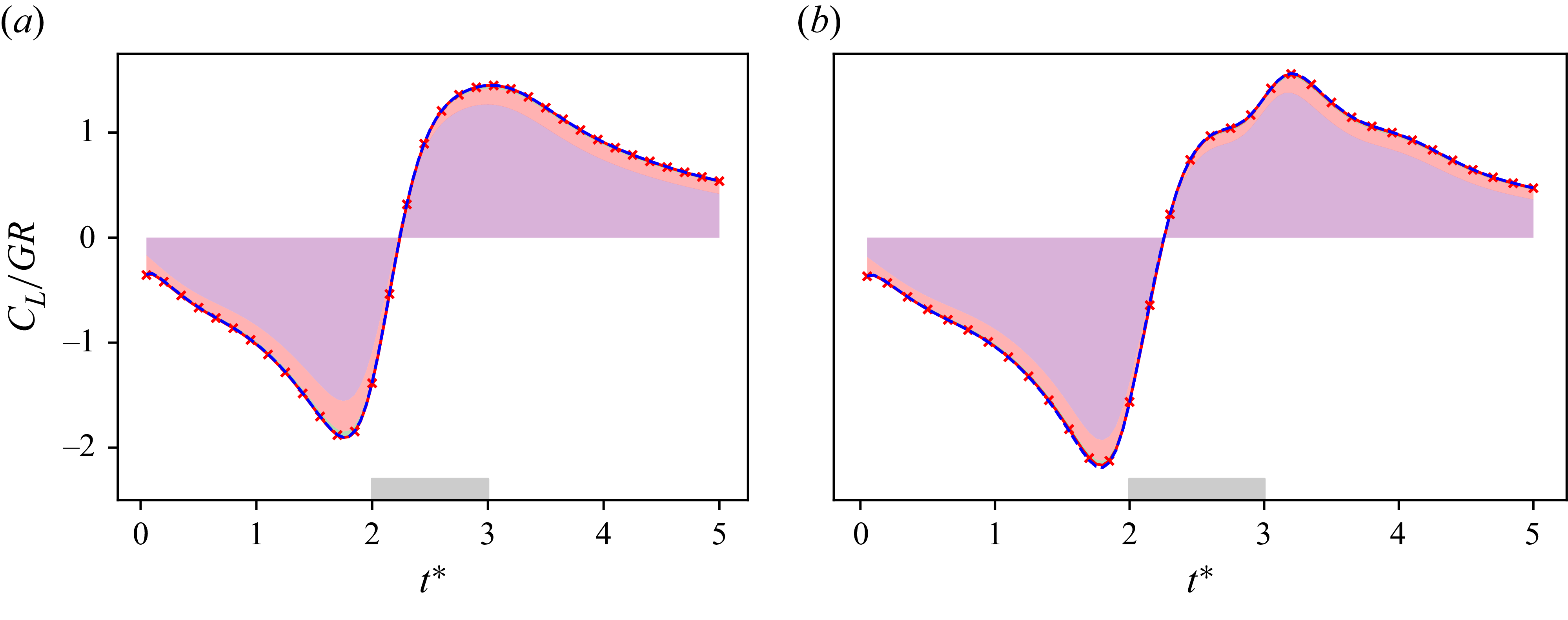
Figure 4 shows the uncontrolled lift coefficients for
 ${\textit{GR}}=0.2$
and
 $0.8$
. For the two cases, it is first verified that the lift obtained with the FPM and shear stress integration is equal to that obtained by integrating pressure and shear stresses at the airfoil surface. Furthermore, it is shown that the lift is, to leading order, governed by the integration of the second term (
 ${\textit{II}}$
) in (3.3), referred to as vortex forces (purple filled areas). The third term (
 ${\textit{III}}$
), or viscous forces within the fluid (pink filled areas), has a marginal but non-negligible influence on the overall lift. Similarly, the contribution of shear stress at the airfoil surface on the total lift is here negligible (green filled areas).
Force partitioning analysis of the uncontrolled case with
 ${\textit{GR}}=0.2$
: (a) snapshots of
 $\textit{II}^{{\kern0.5pt}*}$
, (b) the vorticity field and the contours of
 $\phi _{{e}_y}$
. (c) For each region of
 $\textit{II}^{{\kern0.5pt}*}$
, we display in the histograms the lift generated in the
 $i$
th region
 $C_{L,i}^W$
, as well as the overall lift coefficient.

Force partitioning analysis of the uncontrolled case with
 ${\textit{GR}}=0.8$
: (a) snapshots of
 $\textit{II}^{{\kern0.5pt}*}$
, (b) the vorticity field and the contours of
 $\phi _{{e}_y}$
. (c) For each region of
 $\textit{II}^{{\kern0.5pt}*}$
, we display in the histograms the lift generated in the
 $i$
th region
 $C_{L,i}^W$
, as well as the overall lift coefficient.

Lift generation is correlated with flow dynamics in figure 5 (resp. figure 6), where contours of the predominant contribution to the volumic lift field,
 $\textit{II}^{{\kern0.5pt}*}$
, are displayed for gust ratio
 $0.2$
(resp.
 $0.8$
). Red contours contribute positively to lift, while blue contours contribute negatively. The region boundary is a plain line if rotation dominates
 $(Q \gt 0)$
, or a dashed line if strain dominates
 $(Q \lt 0)$
. The integration of
 $\textit{II}^{{\kern0.5pt}*}$
within the contours gives the contribution of a region (i.e. a flow structure) to the overall lift
 $C_L$
, as shown in the figures in the form of histograms. Specifically, the absolute lift contributions from the
 $i$
th region
 $V_i$
is defined as
 \begin{equation} \big |C^W_{L,i}\big |=\left |\iiint _{V_i} \frac {\textit{II}}{1/2 \rho U_{\infty }^2 c}\, {\rm d}V\right |. \end{equation}
These zonal coefficients
 $ |C^W_{L,i} |$
are reported in figures 5 and 6, where their sign is indicated using a red bar if
 $C^W_{L,i} \gt 0$
, and a blue bar otherwise. Snapshots of
 $\textit{II}^{{\kern0.5pt}*}$
are shown at several relevant convective times corresponding to the vortex gust (i) located upstream of the airfoil
 $(t^*=1)$
, (ii) interacting with the airfoil (
 $t^*=2,2.5,2.8$
), and (iii) located downstream of the airfoil (
 $t^*=4.5$
). Vorticity fields
 $\omega ^*=\omega c/U_{\infty }$
are also displayed, together with isolines of
 $\phi _{\boldsymbol{e}_y}$
, where positive and negative values are depicted using plain and dashed lines, respectively.
At
 $t^*=1$
, the vortex centre is located one chord upstream of the leading edge and is thus not visible on the figures. The flow around the airfoil is characterised by two regions dominated by rotation (positive
 $Q$
, labelled 1 and 2) on both upper and lower surfaces, and two regions dominated by strain (negative
 $Q$
, labelled 3 and 4) in the vicinity of the leading edge. Regions 1 and 2 result from the flow circumventing the airfoil, hence undergoing a rotation-like motion. They are located in areas with relatively large magnitudes of
 $\phi _{{e}_y}$
, thus contribute significantly to lift. It is observed that region 2, which develops on the upper surface of the airfoil, has a larger extent than region 1 in both cases,
 ${\textit{GR}}=0.2$
and
 $0.8$
. However, the magnitude of
 $\textit{II}^{{\kern0.5pt}*}$
is larger in region 1, such that the contribution of region 1 to lift is larger than that of region 2 (see histogram). That is, the vortex induces an asymmetry between regions 1 and 2 such that their net contribution to lift is negative. This asymmetry is related to the downwash induced by the vortex, which slightly deviates the incoming flow. This results in the upper displacement of the stagnation point and the concomitant reduction in effective angle of attack, which becomes negative and thus leads to negative lift. The asymmetry is also observed between strain-dominated regions 3 and 4. However, although their net contribution to lift is also negative, their influence on the overall lift is weak compared to regions 1 and 2.
At
 $t^*=2$
, the vortex reaches the airfoil. For
 ${\textit{GR}}=0.2$
, the overall flow structure is not fundamentally altered. Asymmetry is enhanced such that the net lift contribution of regions 1 and 2 is larger in magnitude than at
 $t^*=1$
. However, the net lift contribution of regions 3 and 4 is now positive, and hence, although very weak, slightly counterbalances contribution from regions 1 and 2. Conversely, the flow for
 ${\textit{GR}}=0.8$
drastically changes from
 $t^*=1$
to
 $t^*=2$
. The vortex gust induces a strong downwash, leading to flow separation at the leading edge. As a consequence, an intense LEV forms on the lower surface of the airfoil, observed as red contours on vorticity snapshots, while the upper boundary layer remains fully attached. This flow topology is in line with experimental observations from Biler et al. (Reference Biler, Sedky, Jones, Saritas and Cetiner2021) and Jones et al. (Reference Jones, Cetiner and Smith2022) at
 $\mathcal{R}_e \sim 10^4$
and
 ${\textit{GR}} \sim 1$
. As expected, the core of the LEV has a large negative contribution to lift, as shown by region 1 on the
 $\textit{II}^{{\kern0.5pt}*}$
field. However, this contribution is partially counterbalanced by that of region 4, corresponding to the strain-dominated corona region that develops around the core of the LEV, as recently discussed by Menon & Mittal (Reference Menon and Mittal2021). Regions 2 and 3 are still present on the upper surface of the airfoil and in the vicinity of the leading edge, respectively, but regions 1 and 4 have a much larger contribution to lift. In other words, the LEV drives lift generation through both its rotational core and strain-dominated corona.
At
 $t^*=2.5$
, the relative contributions from regions 1 and 2 for
 ${\textit{GR}}=0.2$
have significantly changed. Region 2 now has a larger contribution to lift than region 1, hence, because the relative contributions from regions 3 and 4 did not significantly change, the overall lift becomes positive. The stagnation point progressively displaces towards the lower surface of the airfoil, indicating that the effective angle of attack becomes positive. This can be understood by the fact that the rear portion of the (clockwise rotating) vortex induces an upwash at the leading edge. Furthermore, region 1 progressively extends towards the trailing edge. Asymmetry between regions 3 and 4 is also observed, contributing weakly to the positive response in lift to the vortex gust. For
 ${\textit{GR}}=0.8$
, LEV shedding is observed, which we here identify as a discontinuity in the rotation-dominated region below the airfoil. That is, the vorticity-feeding region at the leading edge (region 1) is no longer connected to the LEV core (region 5). Interestingly, shedding appears correlated with an almost zero net contribution to lift from the LEV. The LEV core and corona have almost equal but opposite contributions, and the feeding shear layer has a negligible effect: this yields an overall zero net contribution to lift since all contributions cancel out. Consequently, at this instant, lift principally arises from region 2, which develops on the upper surface of the airfoil as a thick (blue) vorticity layer. Similarly to the case with
 ${\textit{GR}}=0.2$
, the stagnation point displaces to the lower surface of the airfoil, indicating that the local effective angle of attack (at the leading edge) is positive, and consequently the resulting lift is found to be positive.
At
 $t^*=2.8$
, for
 ${\textit{GR}}=0.2$
, a portion of region 1 is shed. This portion, identified as region 5, is located approximately 2.8 chords away from the initial location of the vortex gust, and can hence be considered as the vortex gust itslelf after having interacted with the airfoil. Partly because of this interaction, the contribution of region 1 to lift decreases from
 $t^*=2.5$
to
 $t^*=2.8$
. Conversely, the contribution of region 2 continues to grow, hence the overall lift continues to increase, approaching its maximum at this instant (see figure 4). For
 ${\textit{GR}}=0.8$
, the LEV has been advected towards the trailing edge, and its net contribution to lift (from both its core and corona) is still negligible. Similarly to
 $t^*=2.5$
, lift is driven by region 2, whose strength remains approximately constant.
At
 $t^*=4.5$
, the flow structure for
 ${\textit{GR}}=0.2$
progressively relaxes to a symmetric state consisting of the four regions identified at
 $t^*=1$
. Slight differences in the lift contributions of region 1 and 2 still exist, leading to a relatively small, positive overall lift (regions 3 and 4 having almost equal but opposite contributions). This is again consistent with the airfoil being located in the upwash region of the vortex. For
 ${\textit{GR}}=0.8$
, flow asymmetry persists, with region 2 lifting off the airfoil surface, contrasting with region 1, which develops close to the surface. Positive lift principally arises from the net contribution of regions 1 and 2.
Overall, the above scenario reveals two types of interactions characterised by dominant long-distance effects (at
 $t^*=1.0, 4.5$
) or dominant local interactions (
 $t^*=2.0, 2.5,2.8$
). When long-distance effects dominate, variation in effective angle of attack can be related to
 $\arctan ({\textit{GR}}) \approx {\textit{GR}}$
within the small-angle approximation. Since lift is proportional to the angle of attack for small angles, the lift response is proportional to
 ${\textit{GR}}$
. This explains why
 $C_L/{\textit{GR}}$
curves obtained for
 ${\textit{GR}}=0.2$
and
 $0.8$
collapse for
 $t^*\lt 1$
and
 $t^*\gt 4.5$
(see figure 3 for further evidence). Conversely, when local interactions dominate,
 $C_L$
is no longer proportional to
 ${\textit{GR}}$
, and nonlinear effects induce different
 $C_L/{\textit{GR}}$
responses to vortex gust interaction. These include massive flow separation and LEV formation and shedding.
4.3. Flow physics in controlled cases
Reported results are those obtained for an airfoil submitted to control laws achieving
 $\overline {\eta }=0.88$
for
 ${\textit{GR}}=0.2$
, and
 $\overline {\eta }=0.95$
for
 ${\textit{GR}}=0.8$
. Furthermore, we restrict our analysis to the field
 $\textit{II}^{{\kern0.5pt}*}$
, as it was found to be predominant compared to
 $III^*$
in the uncontrolled case. Similarly, the added mass effect (
 $I$
) is found to be negligible on the overall lift. The predominant volumic lift field
 $\textit{II}^{{\kern0.5pt}*}$
is displayed in figures 7 and 8 for cases with
 ${\textit{GR}}=0.2$
and
 $0.8$
at several relevant convective times. Again, plain contours indicate positive
 $Q$
criterion, and dashed contours indicate negative
 $Q$
criterion. Zonal contributions are also displayed as histograms, along with snapshots of vorticity fields and isocontours of
 $\phi _{{e}_y}$
.
Force partitioning analysis of the controlled case with
 ${\textit{GR}}=0.2$
: (a) snapshots of
 $\textit{II}^{{\kern0.5pt}*}$
, (b) the vorticity field and the contours of
 $\phi _{{e}_y}$
. (c) For each region of
 $\textit{II}^{{\kern0.5pt}*}$
, we display in the histograms the lift generated in the
 $i$
th region
 $C_{L,i}^w$
, as well as the overall lift coefficient.

Force partitioning analysis of the controlled case with
 ${\textit{GR}}=0.8$
: (a) snapshots of
 $\textit{II}^{{\kern0.5pt}*}$
, (b) the vorticity field and the contours of
 $\phi _{{e}_y}$
. (c) For each region of
 $\textit{II}^{{\kern0.5pt}*}$
, we display in the histograms the lift generated in the
 $i$
th region
 $C_{L,i}^w$
, as well as the overall lift coefficient.

For
 ${\textit{GR}}=0.2$
, it was found that the lift coefficient obtained in the control-free case is driven by an asymmetry in the development of upper and lower boundary layers around the airfoil, when the vortex is far from it. In the controlled case, it is shown that this asymmetry vanishes, and that instead, the two boundary layers generate opposite lift contributions of relatively equal amplitude (see figure 7 at times
 $t^*=1.0,2.0,4.5$
). At
 $t^*=1.0$
and
 $2.0$
, the pitch angle is increased such that the stagnation point observed on the upper surface of the airfoil in the control-free case is now located at the very leading edge. In other words, the airfoil aligns with the incoming flow to reach zero effective angle of attack and quasi-zero lift. Similarly, at
 $t^*=4.5$
, the pitch angle is decreased to achieve a similar effect. When the vortex is close to the airfoil and strongly interacts with the boundary layer (see e.g.
 $t^*=2.5$
and
 $2.8$
), it is found that control induces significant changes in flow topology when compared to the control-free case. At
 $t^*=2.5$
, the structure that develops on the upper surface of the airfoil (region 2) is smaller than in the control-free case and is more concentrated in the fore part of the airfoil, hence interacting with lower values of
 $\phi _{\boldsymbol{e}_y}$
, and contributing to a lower value of
 $C^W_{L,2}$
. In addition, a new region with negative contribution to lift develops immediately downstream of this structure, denoted region 5. The latter also contributes to mitigating the effect of the gust (which led to positive lift in the control-free case at this instant), although its contribution is relatively weak. Moreover, region 1 has a larger extent than that observed for the control-free case, which promotes its contribution to negative lift, again mitigating the effect of the gust. It can be seen from the histogram that
 $C^W_{L,1}$
and
 $C^W_{L,2}$
are now similar in magnitude. However,
 $C^W_{L,1}$
is slightly larger than
 $C^W_{L,2}$
, but this difference is partly counterbalanced by the difference in lift contributions from regions 3 and 4 at the leading edge of the airfoil. At
 $t^*=2.8$
,
 $C^W_{L,1}$
and
 $C^W_{L,2}$
are again similar in magnitude, contrasting the control-free case and leading to a relatively low value of
 $C_{L}$
.
For
 ${\textit{GR}}=0.8$
, it has been observed that the lift coefficient is also driven by an asymmetry in airfoil upper and lower boundary layers when the vortex is far from the airfoil. The physical mechanisms underlying control are thus similar to those described for
 ${\textit{GR}}=0.2$
: the airfoil aligns with local flow velocity at the leading edge, as indicated by the stagnation point at
 $t^*=1.0$
, which has moved towards the leading edge when compared to that observed in the control-free case. However, the dynamics of the vortex–boundary layer interaction strongly differs from that of the control-free case. Specifically, while a strong LEV was found to develop on the lower surface of the airfoil, which rapidly shed into the wake, there is no clear evidence of such vortical structure when control is applied. Yet the flow topology remains complex. At
 $t^*=2.0$
, the two vorticity layers on the lower and upper surfaces, denoted as regions 1 and 2, are clearly visible. In addition, the vortex gust, which now has a direct, non-negligible contribution to negative lift, is identified as region 6. Finally, a fourth region with positive lift contribution (region 7) develops in the vicinity of region 1. At
 $t^*=2.5$
, region 2 appears to roll up as an LEV on the upper surface of the airfoil, and a new region with negative contribution to lift, referred to as region 9, develops immediately downstream of it. In addition, the interaction between regions 1, 4 and 7 leads to the partial shedding and advection of region 8 towards the trailing edge. A vorticity layer still exists on the lower surface of the airfoil, referred to as region 1. Region 4 at the leading edge becomes significant. Surprisingly, the overall contribution from all these structures cancels out to reach zero total lift. This demonstrates the ability of DRL to limit lift perturbation by controlling the airfoil, while managing numerous vortical structures with mutual interactions. The same flow complexity is observed at
 $t^*=2.8$
, again with contributions from the vortical structures that sum to almost zero.
At these time instants (
 $t^* = 2.5$
and
 $2.8$
), it is worth noting that the small LEV developing on the airfoil’s upper surface (region 2) has intensified from
 $t^* = 2.5$
to
 $t^*=2.8$
. This strengthened LEV contributes positively to the lift, and in combination with regions 4 and 7, appears to offset the negative contributions originating from regions 1, 3, 8 and 10. This observed behaviour suggests that the DRL agent may promote the formation of this secondary LEV as a control strategy to restore a zero net lift.
5. Conclusion
This paper aims to explain the physical mechanisms behind airfoil–vortex gust interaction and mitigation at low Reynolds numbers. The gust–airfoil interaction is computed by solving the unsteady incompressible Navier–Stokes equations at Reynolds number
 $10^3$
. The control command adjusts the airfoil pitch to minimise lift perturbations on the airfoil. The controller is built as an artificial neural network trained through deep reinforcement learning (DRL). Compared with current literature using local probes as input state, we employ the entire vorticity field as input to ensure the Markov property of the problem. Since classical fully connected networks are not adapted to such high-dimensional input, we include convolutional layers on top of the fully connected layers. These convolutional layers are designed to extract relevant flow features, to guide the fully connected layers when computing the appropriate pitch rate. Our results show that the convolutional-based controller, trained by DRL, effectively mitigates vortex gusts of both medium and large intensity.
The second objective of this work is to identify and understand the underlying physical mechanisms leading to this mitigation. To this end, the force partitioning method (FPM) has been employed to quantitatively assess the amount of lift generated by each flow structure. For uncontrolled medium-intensity gusts, force partitioning reveals a strong asymmetry between the upper and lower airfoil surfaces. This asymmetry is caused by the long-distance effect of the vortex. The short-distance effect is characterised by the detachment of the lower boundary layer due to the vortex core. In the controlled case, the pitch control function balances the lift produced by both the upper and lower surfaces, so that they cancel out to achieve zero net lift.
For higher gust intensity, the uncontrolled lift coefficient is still driven by an asymmetry in the airfoil upper and lower surfaces when the vortex is far from the airfoil. However, the dynamics of the vortex–airfoil interaction is significantly different. When the vortex reaches the leading edge, the lower vorticity layer detaches and forms a strong leading-edge vortex (LEV), which is accompanied by the formation of a strain-dominated corona enclosing the LEV. As the LEV is advected to the trailing edge, the net contribution of the vortex–corona duo tends to zero, and the overall lift is driven by the upper vorticity layer. When control is applied, the lower vorticity layer remains attached, while the upper vorticity layer rolls up into an LEV, accompanied by its strain-dominated corona. Subsequently, the controller is able to pitch the airfoil accordingly to balance the lift induced by the vortex–corona duo and maintain a quasi-zero lift coefficient.
This study demonstrates the capability of DRL to effectively control complex fluid flows. Although DRL control actions are not inherently interpretable, the FPM enables the reverse engineering of the learned strategies. This provides valuable insights into the underlying physical mechanisms driving the control.
This work establishes milestones that can be developed further in future studies. First, it would be interesting to develop a controller that can generalise to a broader range of scenarios representing actual flight conditions. These scenarios could include an extended range of gust ratios, vortex core sizes and vortex offsets. Second, future research could incorporate the volumetric lift field obtained through force partitioning into the controller’s input. This could potentially improve the results. Third, examining a configuration at Reynolds number
 $10^5$
would confirm or refute the validity of the physical mechanisms identified in the present study at higher Reynolds numbers.
Declaration of interests
The authors report no conflict of interest.
Author contributions
Conceptualisation: B.M., T.J., E.R., M.B. Funding acquisition: T.J., M.B. Investigation: B.M. Methodology: B.M., T.J., E.R., M.B. Software: B.M. Validation: B.M. Visualisation: B.M. Writing – original draft: B.M., T.J., E.R., M.B. Writing – review and editing: B.M., T.J., E.R., M.B. All authors approved the final submitted draft.
Appendix A. Mesh and time step convergence
In this appendix, we present the mesh and time step convergence of our simulation. The characteristic mesh cell size is derived from the viscous core radius
 $r_c$
as
 $\delta =r_c/N$
, where
 $N$
is an integer. The time step is derived from the characteristic convective time
 $c/U_{\infty }$
as
 ${\rm d}t=c/(U_{\infty }N_t)$
, where
 $N_t$
is an integer.
Hyperparameters.

Mesh and time step convergence: (a) time step convergence for
 $N=10$
and
 ${\textit{GR}}=0.2$
; (b) mesh convergence for
 $N_t=80$
and
 ${\textit{GR}}=0.2$
; (c) time step convergence for
 $N=10$
and
 ${\textit{GR}}=0.8$
; (d) mesh convergence for
 $N_t=80$
and
 ${\textit{GR}}=0.8$
.

In figure 9, we show the time evolution of
 $C_L/{\textit{GR}}$
as a function of convective time for several tuples
 $({\textit{GR}},N,N_t)$
. In figure 9(a,c), we show
 $C_L/{\textit{GR}}$
with
 ${\textit{GR}}=0.2$
(resp.
 ${\textit{GR}}=0.8$
), for
 $N=10$
and
 $N_t=80,160,320$
. In figure 9(b,d), we show
 $C_L$
, with
 ${\textit{GR}}=0.2$
(resp.
 ${\textit{GR}}=0.8$
), for
 $N_t=80$
and
 $N=5,10, 20$
. It can be seen that the lift coefficients for
 ${\textit{GR}}=0.2,0.8$
converge for each characteristic cell size. And the lift coefficients for
 $N_t=160$
and
 $N_t=320$
are similar, but a slight deviation is observed for
 $N_t=80$
around the local extrema. The rest of the simulation results presented in this paper are obtained with
 $N=10$
and
 $N_t=80$
. We accept this small deviation in order to limit the cost of the simulation and thus achieve a longer controller training.
Appendix B. Network architecture and training hyperparameters
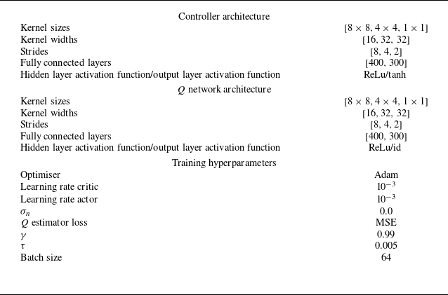
To complement the DRL approach formulated in § 3.1, we present here the network architectures and training hyperparameters in table 2.
The controller and the
 $Q$
estimator are modelled as three convolutional layers followed by two fully connected layers. The convolution layers have decreasing kernel and stride sizes, and increasing numbers of feature maps. The two fully connected layers have 400 and 300 neurons, respectively, where the activation function is the rectifier linear unit (ReLu).
The training hyperparameters are similar to those provided by default in the Open AI Spinning up DRL library.