Many scholars trace the historical origins of monoculture to the settlement of the American grasslands. Western settlement is typically portrayed as a process driven by single-crop farming. Historians describe how wheat cultivation disturbed fragile grasslands and marginal lands were plowed, leading to the emergence of the Dust Bowl.Footnote 1 Most accounts are based on aggregate data and references to disparaging views of farmers' use of crop rotation, manure, and cover crops in contemporary writings by soil scientists, agricultural economists, and conservationists.Footnote 2 Economic historians regard the pace of change as more measured, arguing that the institutional framework of settlement and slow diffusion of new technology constrained the development of large farms.Footnote 3 Recent work by Geoff Cunfer also suggests that settlers moved on to the Great Plains in a deliberate way, while developing and maintaining diverse practices.Footnote 4
Looking back, it is clear American agriculture stood at an ecological frontier in the 1930s. With new and better machinery, more farms than ever before were poised to become thousand-acre enterprises. When they did, the largest of farms began a process that would profoundly reshape rural communities and agricultural landscapes. Progressive Era economists welcomed the increasing scale of farming, seeing it as a way to close the gap between rural and urban incomes.Footnote 5 Over the long run, rural incomes were boosted.Footnote 6 But as agronomists and soil scientists warned along the way, the shift toward monoculture displaced many of the beneficial practices that maintained and restored arable land in past centuries.Footnote 7 While cereal productivity has more than doubled since the 1930s, the continuous cropping made possible by synthetic fertilizer also diminished the “planned” diversity of cropping systems. Ecologists warn of the harmful effects. Increased reliance on fertilizer, irrigation, and pesticides has led to soil erosion, and the pollution of groundwater, rivers, and lakes. The simplification of crop systems has adversely affected the composition and abundance of beneficial insect, invertebrate, and microorganism populations essential to plant and soil processes.Footnote 8
This article addresses competing claims about the impact of growing farm scale on crop diversity during the era of mechanization. One is that increases in farm scale led to monoculture and environmental degradation and the other is that the adoption of new technology and the expansion of farm sizes were limited during the period before 1945. Both are investigated here by testing the relationship between farm size and crop diversity using a new sample of the Kansas State Census of Agriculture. The data include repeated farm observations and cover 25 townships between 1875 and 1940.Footnote 9 Judging by the crop statistics reported by 25,123 farms, the drive toward specialization met a lukewarm reception in Kansas.Footnote 10 Even in the heart of the Dust Bowl, farmers' land use choices were remarkably varied. The analysis suggests that the great majority of midsized farms expanded the diversity of their farms over time, while very large farms and small farms became more specialized. As farmers reached midlife, the diversity of crop choices peaked, as parents took advantage of the maturing labor power of their children, and then fell as young adults moved away, leaving parental homes with too little labor to maintain the diverse land use.
DATA AND METHODS
The aim of the study is to develop models where repeated observations are nested in a multilevel framework with the environmental context formally specified in the model. The spatial distribution of the townships must capture meaningful variation in environmental conditions across the state: in precipitation, temperature, soil quality, topography, native vegetation, and agricultural potential. Rather than a randomized design, target counties are identified based on a chessboard pattern, maximizing spatial reach and biophysical variation, and the selections included are based on the availability of the census data. Townships are excluded if the land in the township was part of a military base, urban area or Indian reserve, or census data were missing. Townships are included if they remained predominantly agricultural and if they had the highest rural population density in 1910. We assumed that farmers and farm families gravitated to the most promising landscapes within each county, and that by selecting the most densely settled rural townships, the sample was weighted toward areas with higher proportions of arable land.
The spatial distribution of townships is shown in the map in Figure 1. Surrounding the townships, highlighted in black, are county boundaries and a regional classification of land use developed by Kansas State Agricultural Extension staff in 1933.Footnote 11 The zones reflect many enduring
SAMPLE TOWNSHIPS AND THE FIVE AGROECOLOGICAL ZONES

patterns. The Kansas Corn Belt, then and now, lies in a tier of counties situated in gently rolling, glaciated hills along the northern boundary with Nebraska. Mixed farming was practiced within a series of ridges or escarpments, known as the Osage Cuestas, along the eastern parts of the state south of the Kansas River. Further west, a bluestem pasture region, known as the Flint Hills, is situated on Permian-age limestones and shales. Because the uplands have thin soils and contain numerous bands of flint, even the most permeable soils are full of gravel, from the weathering of limestone. Today, large portions of the region remain in grassland cover, and serve mainly as pasture. The central Wheat Belt lies in the High Plains geologic region in the center of the state where the terrain is level, rainfall averages 32 inches per year, and the soils are rich and permeable.Footnote 12 The climate favors winter wheat production because of long, cool, wet springs, followed by dry warm periods for fruiting and harvesting. None of the problems associated with hot, humid environments, such as lodging, rust, or excessive straw, affect wheat grown in Kansas.Footnote 13 Along the state's western boundary with Colorado annual rainfall is close to the minimum of 15 inches of rain needed for wheat cultivation; therefore farmers raised cattle, grew wheat, and incorporated the drought-resistant feed crop, sorghum, into their crop regimes.
The data are examined through two main lenses. An overview of trends in farm diversity and farm scale are presented using the data as conventional cross sections. Then longitudinal trends are analyzed using observations linked over time. The basic data task in linking cases longitudinally was to accurately match persons listed on the agricultural and population census in the same year, and then use population information to link individuals from one census to the next. Matching the population census to the agricultural census in the same year was the most straightforward exercise. Most individuals listed in the agricultural censuses were farmers and adult males and listed in the same order as households in the population census. To link individuals over time, a wider set of information—name, birth order, age, marital status—was used. Linkage rates within the same census year were consistently high, averaging 86 to 95 percent within each township. Over time, linkage rates were lower because of outmigration, mortality, and other unobserved changes.
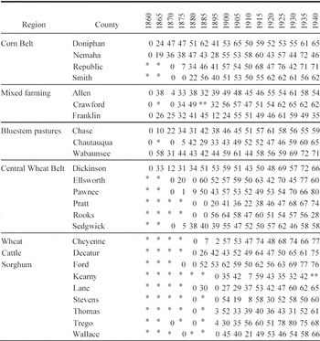
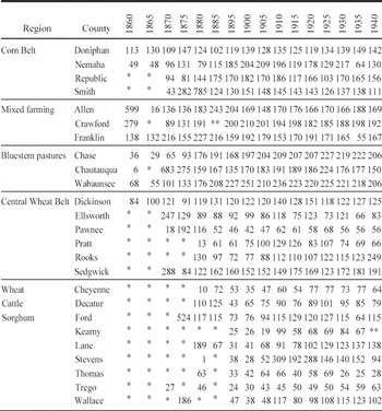
Over the whole length of the study period, the turnover in farm operator population was substantial. A total of 14,022, or 56 percent, of the sample farms were observed only once in the data set after 1875. Much of the high turnover occurred within the first generation of settlement. After the first twenty to twenty-five years, persistence rates increased in each of the study townships. The first table in the appendix shows how the pattern was repeated across the state as settlement progressed westward. The townships are grouped in the table according to the agro-ecological zones illustrated above in Figure 1. The proportions represent the number of household heads still resident in the township from the previous census. The denominator is the number of current households. One advantage of calculating persistence this way, is that the proportions quickly provide a sense of when previously listed heads of household outnumbered “new” heads of household.Footnote 14
CROP DIVERSITY INDEX
At various times, farm experts have argued that farms that produce a variety of plant and animal products are more likely to be successful in the long run. Crop rotations and a balance of land uses (including the right proportion of pasture and grazing activity) were taken by knowledgeable observers as signs that farmers took the necessary steps to maintain the productivity of arable land. Before the arrival of inorganic fertilizers, this balance was essential to what many eventually referred to as “permanent agriculture.”Footnote 15 To create a summary measure that reflects the varying balance of land uses employed by farmers to sustain production, I use an inverted Herfindahl index similar to the one used by Cunfer.Footnote 16 The traditional normalized Herfindahl index applied to crop mix would be the sum of the squared values of the shares of land devoted to each crop:

where si is the percentage of land devoted to crop i and n is the number of crops. The normalized H index has a value of one if only one crop is produced on the farm and is reduced as more crops are produced and shares of land devoted toward each crop are more evenly distributed.Footnote 17 To convert the index so that one is the highest level of diversity and zero the lowest, I use the formula:

where N is the number of crops. In this case, I chose eight major land uses to represent the key components of Kansas agriculture: wheat, corn, oats, rye, barley, sorghum, hay, and pasture.Footnote 18 Hay includes several soil building crops and grasses: alfalfa, blue grass, clover, orchard grass, brome grass, timothy, red and alsike clover, sweet clover, lespedeza, cowpeas for hay, and soy beans for hay, although Kansas did not report the same information from census to census. Various forms of hay were sown to arable land to rest it, rebuild organic matter and restore soil nitrogen, as well as to provide feed for livestock. Oats were mainly used as a feed crop for horses, but were sometimes sown in the fall to serve as a winter cover crop, and plowed under in the spring as a green manure. The pasture category provides a measure of the degree to which farmers used land for grazing of livestock. If the farmer evenly divided his acreage so that 12.5 percent of the farm was used to produce each of the 8 crops, D equals one. If the farmer produced only one crop, D equals zero.Footnote 19
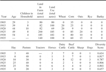
To illustrate how the crop diversity index summarizes the activities on an individual farm, consider the farm of Frank and Elizabeth Marnell located in Grant Township, Crawford County, Kansas in Table 1. In 1905 Frank was 29 years of age and operated a small farm with 35 acres in corn, 5 acres in hay, and 40 acres devoted to pasture for 3 horses and 7 dairy cows, leading to a crop diversity index of 0.634. By 1925 the middle-aged Marnells and their 10 children had expanded the farm to 200 acres and increased the crop diversity index to 0.806 with 40 acres of land in pasture, 85 in corn, 20 in oats, 15 in sorghum, and 25 acres devoted to hay. As the couple aged further and the children left the farm, the number of crops and livestock declined and the crop diversity score fell to 0.657 by 1935.
FARM OF FRANK MARNELL, GRANT TOWNSHIP, CRAWFORD COUNTY, KANSAS, 1905-1930

Notes:
Diversity score calculated as an inverted normalized Herfindahl index.
Source:
Household responses from microfilm manuscript census (federal and state) returns, 1905-1935.
ARM SCALE AND DIVERSITY
With so much emphasis on large wheat farms in the literature, it is surprising to learn that only about 40 percent of the farms in the sample exceeded the dimensions of the homestead sized farm (160 acres) during the period. Most farms in the sample were midsized operations between 160 and 319 acres. Farms larger than 320 acres represented no more than 13 percent of farms from about 1905 to 1940. In the western regions, however, the half-section farm (320-479 acres) grew over time to represent about 25 percent of farms. Because of the semi-arid conditions, viable farms needed to be larger. Less than 10 percent of farms in the more intensively cropped Wheat Belt graduated to the three-quarter section (480-639 acres) sized farm. The latter were more likely to emerge in the far west, where cattle-raising was often combined with crop farming. In the High Plains, the three-quarter section and section-sized farms represented a third or more of all farms. Again, with the emphasis on beef cattle in the literature, it is surprising to learn that dairy cattle were a big part of the average farm in the far west after “dirt” farmers moved into the region. During the era between 1905 and 1940, about one-quarter of the dairy animals reported in the sample townships were on farms in the far west. The fodder requirements help to explain why pasture and native grassland were generally about half of reported land use activity. But tillage remained diverse as well. In the Wheat Belt, where the proportion of pasture was generally not much more than a quarter or a fifth of reported land use, tillage became less diverse after 1905. The lack of balance in arable crop systems was most evident on farms a half-section or more in size, particularly in the western regions.
The massive wheat farm of regional legend was rare in the data. Only 682, fewer than 3 percent, of 25,123 farm observations in the sample reported 320 acres or more in wheat cultivation. Only 164 farms reported planting more than 480 acres of wheat, and only 54 reported a section-sized (640 acre) or larger wheat crop. These farms accounted for only 7.4 percent of all reported land in farms. Virtually all large wheat crops were located in the far west of the state in Cheyenne, Decatur, Ford, Kearny, Lane, Stevens, Thomas, and Wallace counties with the exception of 4 farms reporting more than 640 acres in wheat in Pratt county—just east of the far western zone.
The large wheat farms were often operated by farmers who arrived after the frontier stage was over, and their operations were focused on short-term returns. The first thousand-acre plantings of wheat, for instance, were reported in 1920 in two western counties, Thomas and Stevens. All were newcomers from the Upper South who arrived between 1910 and 1920 and were no longer listed after 1925. The longest-resident thousand-acre wheat farm proprietor was Virginian Edgar Gano, who arrived in Lane County sometime before the 1920 census. At first, the mainstay of his 3,800 acre farm was a herd of 250 beef cattle. By 1930 Gano reported only 30 head of cattle and sowed a 1,600 acre wheat crop, planted 150 acres in sorghum, cultivated 40 acres in hay, and left 3,000 acres in pasture.
A few corporate farms also were established before the state voted to ban corporate farming in 1931. One of the largest was the Wheat Farming Company, which cultivated 60,000 acres in 1930 with a fleet of thirty combines.Footnote 20 One of its farms in Wallace County listed 7,690 acres and reported no livestock or pasture while sowing 4,920 acres to wheat, 320 acres to corn, and 1,850 acres to sorghum. By 1935, after the ban on corporate farming, no listing for the company appears in the township's returns.Footnote 21
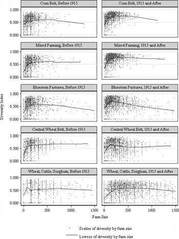
The relationships between diversity and farm size for several land use regions and two time periods can be seen in the series of scatter plots in Figure 2. The graphs illustrate the broad range in size distributions of observations (along the x-axis) in the two western zones, as well as the more compressed density around midsized farms of observations in the eastern regions. Before 1915 the relationship between scale and diversity is quite flat, as the horizontal trajectory of the Lowess smoothing function illustrates. After 1915 larger farms are associated with lower levels of diversity, and declines in the Lowess smoother are pronounced in each region, particularly after farms reach sizes larger than a half-section (320 acres). In the far west, the decline isn't noticeable until farms are larger than a section (640 acres). The other pronounced difference in the panels (from left to right) is the rise in average levels of diversity in the period after 1915. The higher levels are especially visible in the Lowess smoother in the three eastern regions.
The scatter plots show that there was a core of mid-sized farmers who chose diverse production as part of a process of local adaptation. As settlers transferred knowledge to new settings and experimented with local conditions, they chose more diverse crop mixes. The emphasis on diversity increased after 1915. Diversity made economic sense to this core farm population because its time horizons were broader than a few harvest seasons.
Historians and economists have suggested that the diversity results in part from risk aversion, often defined as a safety-first orientation.Footnote 22 To this majority or core population, sustaining production, conserving resources, and reducing risk of crop failure were preferred to the risks that came from specialization. Diversity helped to achieve more consistent returns, by guarding against the failure of particular crops, especially in a semi-arid environment prone to wide seasonal variations and periods of drought. At the same time, new technology and increasing farm scale were having an impact. The introduction of the tractor did not immediately overturn a safety-first orientation—few
TWOWAY SCATTER OF DIVERSITY AND FARM SIZE, WITH LOWESS SMOOTHER, BY LAND USE ZONE AND PERIOD

abandoned livestock with the arrival of mechanized plowing, harrowing or seeding—yet there were very large farms that staked most if not all of their potential gains on a few key crops or land uses. Increases in scale were a sign of things to come.
ANALYSIS
This final section evaluates the long term trend toward diversity in a repeated measures model. The data are appropriate for panel data or fixed effects designs. The data represent a clustered longitudinal sample, in which there are multiple years reported for each farm, nested within township level clusters. Each township has a different number of units of analysis and a different number of time points at which the outcome is measured. Thus the data set is unbalanced. I fit a fixed effects model that estimates diversity without any higher level covariates and then include a time-invariant township-level covariate in the final model, as a control for an interaction term.
In the panel design, I estimate the relationship of the diversity index, Dijt, for farm i in township j in year t. In the full model, I estimate

where Xijt is a vector of variables describing land use practices chosen by farm i in township j in year t, including measures of farm size, the presence of livestock, crop choices, and the presence of a tractor (available only between 1915-1935); Zijt is a vector of household characteristics of farm i in township j in year t, including the age of the household head, age squared, the number of the children in the household and that number squared; Pijt -1 is a zero-one dummy for persistence of farm i in township j that has a value of 1 when the family was there in the prior time period, and zero if they were not; Rj is a zero-one dummy for whether the farm was located in the Wheat Belt region. I also estimate several fixed effects, including a vector fj of effects for each farm, a vector of time fixed effects (with a dummy variable representing each year in the sample) and an error term eijt.
RESULTS
The estimates in Table 2 are presented in four model specifications. Descriptive statistics of the variables used in the analysis are provided on the left. Because farm size is used as a categorical variable, overall
FIXED EFFECTS ESTIMATES OF DIVERSITY INDEX

*** p < .001
** p < .05
* p < .10
Note:
Dependent variable is diversity index.
Sources:
Manuscript state and federal agricultural and population censuses.
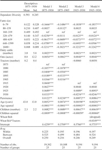
proportions are reported in the means column. Otherwise, the units are specified in parentheses. The first model uses all observations from1875 to 1930, the second and third models partition the observations in 1915 to illustrate change over time, and the fourth introduces an interaction term to emphasize the uneven diffusion of mechanization.Footnote 23
The farm size coefficients show that the smallest and largest farms were significantly less likely to maintain diverse production. The diversity index is 0.167 to 0.186 points lower for farms less than 80 acres relative to the reference group of 160-319 acres. As farms increased in size from the reference group, the diversity index dropped. Farms larger than 1600 acres had diversity indexes that were an estimated 0.30 to 0.32 points lower across the four model specifications.
The presence of dairy cattle was one sign that farms were pursuing more diverse land use and the planting of oats was a crop choice that was strongly associated with balanced land use. The time effects in model 1 demonstrate how diversity increased over time in the sample population, from an estimated low in 1880 (0.106 index points below the reference year) to successively higher levels, beginning in 1905 and continuing through 1930.
Diversity is also strongly affected by the point at which land use decisions were made in the farmer's life cycle and by the number of children (defined as persons under 21 years of age) in the household. In this case, the relationships are not linear. They follow a curvilinear pattern, increasing into midlife and then declining as heads of household transferred productive assets to offspring and farmed less actively in later life. This rise and deceleration in diversity during the life cycle is captured in the models by the introduction of quadratic terms for age and the number of children. These phenomena are consistent across the farm population, reflecting the tendency for farms to take advantage of the growing labor power of maturing children, to increase the variety of productive activities, and presumably to stabilize incomes and manage risk. The estimates are different after 1915 than before. The coefficients for age in model 2, for instance, predict that diversity will rise until the head of household reaches age 50.2 [0.0074/(2 × 0.00001) = 50.2] before beginning to decline, and that diversity will peak when there are 5.3 children [0.00887/(2 × 0.00083) = 5.3] in the household.
After 1915 the predictions for age and children in model 3 indicate that peak diversity arrives at a younger age [0.00198/(2*.00003)=39.1], but that diversity still peaks when there are 5.2 children in the household [.00617/(2 × .00059)=5.2]. After 1915 young farmers began their careers at higher initial levels of diversity (as the scatter plots in Figure 2 suggest) and maintained higher levels of diversity throughout their farm careers (which helps to explain the flatter time trend after 1915). Those who were prior residents of the study communities were the only ones to pursue higher diversity than their neighbors (as the small but statistically significant parameter for residential persistence suggests). But the overall growth trend reached a plateau after 1915, dipping slightly in 1930, as the time estimates in models 3 and 4 illustrate.
The tractor had the potential to reduce diversity by allowing the farmer to harvest larger fields of the same crop. The estimates in model 3 for 1915 through 1930 indicate that the presence of a tractor led to lower diversity, but the relationship is not statistically significant. A common explanation offered in the literature is that the adoption was uneven and early diffusion of tractors in this data confirms and extends the observation.Footnote 24 In fact, tractors appeared to reinforce existing land use practice rather than reshape it. The exception occurred mainly in the so-called Wheat Belt region, where crop production was more intense and less land was reserved for pasture and grazing. In that region, the adoption of tractors had an unambiguously negative impact on diversity. When an interaction term for number of tractors and a dummy variable for the Wheat Belt region were added, the main effect for tractors changes direction, while the interaction term predicts a -0.0349 (significant at p < .001) drop in diversity for every tractor reported in the Wheat Belt region.Footnote 25
Within, between, and overall R-squares are part of the standard output in fixed effects designs, and are reported in Table 2. The goodness of fit reported (in “xtreg, fe”) is closest to an ordinary OLS in its estimate of the within R 2since the other estimates of between and overall fit are calculated simply as correlations squared.Footnote 26 What they suggest is that the models do a much better job of predicting the between township variance than the within farm change. Or to frame it another way, as much as farmers favored higher diversity over time, far more variance in overall levels of diversity derived from the choice of where to farm, in the beginning.
CONCLUSIONS
Was diversity growing over time? Yes, the overwhelming direction of change was for diversity to increase. Although the signs of greater specialization and monoculture are visible in these returns, they did not shape the behavior of the majority. No doubt, the growth in diversity had slowed by the 1920s and 1930s. But the impact of mechanization was limited to the select few who made the largest investments. For most farms, technological change largely reinforced existing preferences, and those preferences continued to be shaped by the life cycle and the size of the household. What is also striking is the degree to which these choices were shaped by the environments in which farm households chose to settle.
In the end, farmers generally ignored the drive toward specialization promoted by the state and agricultural reformers in the early twentieth century. When farms in the central plains broke through scale barriers that governed family farming in the eastern United States, they did not abandon the diverse production that had sustained smaller-scale production in earlier centuries. There were short-lived farm enterprises that fit the mold of “wheat mining” operations. But most farms were not practicing fencerow to fencerow monoculture. The sheer density of mid-sized farms practicing an increasingly balanced agriculture is the most stunning finding of this research. Specialization was not widespread in the years leading to the Dust Bowl in Kansas. Instead diversity remained central to ways in which family farms sustained themselves. Although many stood on a new ecological frontier, few chose to cross it.
Appendix
LINKING
The links were made by applying a hierarchy of matching algorithms in multiple passes. An interface developed in Java allowed users to retrieve data tables stored in Oracle and display them side by side. Beginning with the strictest algorithm, the user applied a SQL query based on an exact match of first and last name. All the possible matches for the criteria were then displayed on the right-hand side. Matches at lower levels of likelihood were also invoked using a form of “stem” matching, created by removing duplicate consonants and all vowels.Footnote 27 Generation of the stems allowed users to filter through variations in the spelling of names and interpretations of the handwritten manuscript records. Records were then sorted by propensity scores, and users evaluated associations with a score of 50 or more for manual linkage. Once a match was identified and chosen by the user, by clicking rows in left and right hand tables, the user was prompted to confirm the link in a dialogue box. A “make link” box allows users to specify whether a person linked over time between population censuses was part of a family, based on the household information on other family members visible on both sides. All the individual links are then stored for the members of the household meeting the match criteria.
Subdivided by age and sex, the pools of potential links were quite small. Often nominal information was enough to make the necessary distinctions between persons within the same agricultural townships. In the years where the population information is derived from a state census—1865, 1875, 1885, 1895, 1905, 1915, and 1925—the order of households was also the same on both schedules. Linkage rates within the same census year were typically very high. The cells with a single asterisk in Appendix Tables 1 and 2 indicate where census information was not yet available in the early years of settlement and the cells with a double asterisk indicate where information is missing, in Crawford in 1885 and Kearny in 1940.
The first availability of the census data is indicated by the first zero in each row. Subsequent zeros, in Smith, Pratt, Rooks, Lane, Stevens, Trego, and Wallace, indicate that no former residents linked forward in time. Expressed as a proportion of the current population in Appendix Table 1, the persistence rates also minimize the effect of boundary changes. Often the formation of townships took place after the first census. High population counts in Appendix Table 2 (see below) for Allen in 1860, Chautauqua in 1870, Ellsworth in 1870, Sedgwick in 1870, Ford in 1875, Stevens in 1910 and 1920, and Wallace in 1875, reflect the data gathering strategy. In cases where boundary information was uncertain, census data was gathered from the whole county in order to maximize forward linkage. This also elevated the numbers of cases that were never tracked forward from one census to the next because they fell outside of the boundaries of new, smaller townships. After boundaries stabilized, this attrition is eliminated.
HEADS OF HOUSEHOLD STILL RESIDENT FROM PRIOR CENSUS, AS A PROPORTION OF CURRENT HOUSEHOLDS, 1860-1940

**Missing data
*Township not formed
Sources:
Manuscript state and federal population censuses, 1860-1940.
COUNT OF HOUSEHOLDS, BY CENSUS YEAR

**Missing data
* Township not formed
Source:
Manuscript state and federal censuses, 1860-1940.