2.1 Problem statement

Figure 1.

Definition sketch of the wave radiation problem by a half-submerged sphere of radius $r_{1}$ which oscillates vertically with an amplitude of $a$ at a frequency of $2\unicode[STIX]{x1D714}_{0}$ in deep water. A circular cylindrical coordinate ($r$, $\unicode[STIX]{x1D713}$, $z$) system is defined to describe the problem. The fluid domain is represented as ${\mathcal{D}}$ that is encircled by the body surface $S_{B}$, the free surface $S_{F}$, the far-field vertical cylindrical surface $S_{\infty }$ at $r=r_{2}\gg r_{1}$, and the fictitious deep-water surface $S_{0}$.

We consider the hydrodynamic problem of nonlinear capillary–gravity wave interaction with a floating sphere in deep water in the context of potential flow. The problem is depicted in figure 1. The sphere with radius $r_{1}$ is half-submerged and undergoes a periodic vertical oscillation with amplitude $a$ and frequency $2\unicode[STIX]{x1D714}_{0}$. At any time $t$, the velocity potential $\unicode[STIX]{x1D719}(r,\unicode[STIX]{x1D713},z,t)$ that is used to describe the fluid motion satisfies the Laplace equation in the fluid ${\mathcal{D}}(t)$,

(2.1)$$\begin{eqnarray}\unicode[STIX]{x1D6FB}^{2}\unicode[STIX]{x1D719}=0\quad \text{in }{\mathcal{D}}(t),\end{eqnarray}$$

where $\unicode[STIX]{x1D735}\equiv (\unicode[STIX]{x2202}/\unicode[STIX]{x2202}r,\unicode[STIX]{x2202}/r\unicode[STIX]{x2202}\unicode[STIX]{x1D713},\unicode[STIX]{x2202}/\unicode[STIX]{x2202}z)$ and $t$ represents time. The kinematic and dynamic boundary conditions on the instantaneous free surface $S_{F}(t)$ are

(2.2)$$\begin{eqnarray}\unicode[STIX]{x1D701}_{t}+\unicode[STIX]{x1D735}\unicode[STIX]{x1D701}\boldsymbol{\cdot }\unicode[STIX]{x1D735}\unicode[STIX]{x1D719}=\unicode[STIX]{x1D719}_{z}\quad \text{on }S_{F}(t)\end{eqnarray}$$

and

(2.3)$$\begin{eqnarray}\unicode[STIX]{x1D719}_{t}+\frac{1}{2}\unicode[STIX]{x1D735}\unicode[STIX]{x1D719}\boldsymbol{\cdot }\unicode[STIX]{x1D735}\unicode[STIX]{x1D719}+g\unicode[STIX]{x1D701}+\frac{T_{s}}{\unicode[STIX]{x1D70C}_{w}}\unicode[STIX]{x1D735}\boldsymbol{\cdot }\boldsymbol{n}=0\quad \text{on }S_{F}(t),\end{eqnarray}$$

where $\unicode[STIX]{x1D701}(r,\unicode[STIX]{x1D713},t)$ denotes the instantaneous elevation of the free surface, $g$ is the gravitational acceleration, $\boldsymbol{n}$ is the unit normal vector of the free surface pointing out of the fluid, $T_{s}$ is the coefficient of surface tension of water (in contact with air) and $\unicode[STIX]{x1D70C}_{w}$ is the water density. The boundary condition on the instantaneous sphere surface $S_{B}(t)$ is

(2.4)$$\begin{eqnarray}\unicode[STIX]{x1D719}_{n}=\unicode[STIX]{x1D709}_{t}n_{z}\quad \text{on }S_{B}(t),\end{eqnarray}$$

where $\unicode[STIX]{x1D709}(t)$ represents the vertical displacement of the sphere centre, and $n_{z}$ is the vertical component of the unit normal of the body surface. In the present study, the sphere is forced in harmonic motion with $\unicode[STIX]{x1D709}$ given by

(2.5)$$\begin{eqnarray}\unicode[STIX]{x1D709}(t)=a\sin 2\unicode[STIX]{x1D714}_{0}t.\end{eqnarray}$$

In deep water, the fluid motion vanishes

(2.6)$$\begin{eqnarray}\unicode[STIX]{x1D735}\unicode[STIX]{x1D719}=0\quad \text{on }S_{0}.\end{eqnarray}$$

The radiation condition is imposed at the far-field surface $S_{\infty }(t)$, which requires that the generated waves due to body oscillation propagate outwards. In addition, the initial conditions of $\unicode[STIX]{x1D719}(r,\unicode[STIX]{x1D713},z,t=0)$ on the free surface $\unicode[STIX]{x1D701}(r,\unicode[STIX]{x1D713},t=0)$ and the position$\unicode[STIX]{x1D709}(t=0)$ and velocity $\dot{\unicode[STIX]{x1D709}}(t=0)$ of the sphere need to be specified.

In the context of gravity waves, the above stated initial boundary value problem is complete, for which a unique solution exists (John Reference John1950) because the homogeneous problem (with linearized free-surface boundary conditions) has a trivial solution only. In the context of gravity–capillary waves, the solution of the stated problem is non-unique because the homogeneous problem (with linearized free-surface boundary conditions) possesses a non-trivial solution which is dependent on the radial slope of the free-surface at the intersection line (often known as the waterline) of the sphere with the free surface (Shen & Liu Reference Shen and Liu2019). A unique solution of the stated problem, which represents outgoing progressive ring waves due to forced vertical sphere oscillation, can be achieved only under the condition of zero radial slope of the free surface on the waterline

(2.7)$$\begin{eqnarray}\unicode[STIX]{x1D701}_{r}(r,\unicode[STIX]{x1D713},t)=0\end{eqnarray}$$

for $0\leqslant \unicode[STIX]{x1D713}<2\unicode[STIX]{x03C0}$ at any time (Rhodes-Robinson Reference Rhodes-Robinson1971; Shen & Liu Reference Shen and Liu2019). In general, the position of the waterline varies with time in the time domain simulation. For small body oscillation amplitude $a$, the waterline can be approximated to be fixed at the position $r=r_{1}$. For large body oscillation amplitude $a$, a numerical procedure described in § 3.2 is employed to determine the waterline position in the nonlinear time-domain simulation. Appendix C describes a numerical approach for the determination of the solution of the linearized homogeneous problem (with $\unicode[STIX]{x1D719}_{n}=0$ on the body surface, but $\unicode[STIX]{x1D701}_{r}\neq 0$ on the waterline $r=r_{1}$) in the frequency domain. The homogeneous solution represents the progressive radial cross-waves.

The purpose of this work is to investigate the stability of the finite-amplitude progressive ring waves (forced by a harmonic vertical sphere oscillation) subject to the small disturbance given in terms of the progressive radial cross-waves including both gravity and surface tension effects.

2.2 Instability-analysis method

We write the governing equation of the above stated nonlinear wave–body interaction problem in symbolic form,

(2.8)$$\begin{eqnarray}\frac{\unicode[STIX]{x2202}\boldsymbol{u}}{\unicode[STIX]{x2202}t}={\mathcal{N}}(\boldsymbol{u}),\end{eqnarray}$$

where ${\mathcal{N}}$ is the nonlinear operator of the problem and $\boldsymbol{u}\equiv (\unicode[STIX]{x1D701}(r,\unicode[STIX]{x1D713},t),\unicode[STIX]{x1D719}^{s}(r,\unicode[STIX]{x1D713},t))$ is the solution of the nonlinear problem in which $\unicode[STIX]{x1D719}^{s}\equiv \unicode[STIX]{x1D719}(r,\unicode[STIX]{x1D713},z=\unicode[STIX]{x1D701}(r,\unicode[STIX]{x1D713},t),t)$ represents the velocity potential on the free surface.

In a linear stability analysis, we write $\boldsymbol{u}$ as the sum of a nonlinear base flow $\boldsymbol{u}_{0}$ (corresponding to finite-amplitude propagating ring waves) and a small disturbance $\boldsymbol{u}^{\prime }$,

(2.9)$$\begin{eqnarray}\boldsymbol{u}(r,\unicode[STIX]{x1D713},t)=\boldsymbol{u}_{0}(r,t)+\boldsymbol{u}^{\prime }(r,\unicode[STIX]{x1D713},t),\end{eqnarray}$$

where $\boldsymbol{u}_{0}$ satisfies the inhomogeneous body-boundary condition (2.4) with the zero radial-slope condition (2.7) while $\boldsymbol{u}^{\prime }$ satisfies the homogeneous body-boundary condition $\unicode[STIX]{x1D719}_{n}=0$ but with $\unicode[STIX]{x1D701}_{r}\neq 0$ on the waterline. Substituting (2.9) into (2.8) then leads to the linearized equation governing the temporal-spatial evolution of the disturbance,

(2.10)$$\begin{eqnarray}\frac{\unicode[STIX]{x2202}\boldsymbol{u}^{\prime }}{\unicode[STIX]{x2202}t}={\mathcal{L}}(\boldsymbol{u}^{\prime }),\end{eqnarray}$$

where ${\mathcal{L}}$ is a linearized time-periodic (variable-coefficient) operator given by the Jacobian of ${\mathcal{N}}$ with respect to $\boldsymbol{u}$ (evaluated at $\boldsymbol{u}_{0}$). For the present problem, ${\mathcal{L}}$ has a frequency of $2\unicode[STIX]{x1D714}_{0}$ and a period of $T_{0}/2$, where $T_{0}=2\unicode[STIX]{x03C0}/\unicode[STIX]{x1D714}_{0}$ is the period of the subharmonic.

Since $\boldsymbol{u}^{\prime }$ is periodic in $\unicode[STIX]{x1D713}$, we expand $\boldsymbol{u}^{\prime }$ in a Fourier series

(2.11)$$\begin{eqnarray}\boldsymbol{u}^{\prime }(r,\unicode[STIX]{x1D713},t)=\mathop{\sum }_{m=0}^{\infty }\overline{\boldsymbol{u}}_{m}^{\prime }(r,t)\cos (m\unicode[STIX]{x1D713}),\end{eqnarray}$$

where, without loss of generality, we consider the cosine series in $\unicode[STIX]{x1D713}$, and $\overline{\boldsymbol{u}}_{m}^{\prime }(r,t)$ represents the amplitude of the $m$th cosine mode. In practice, the infinite series in (2.11) is truncated at a suitable large number $M$. Substituting (2.11) into (2.10) gives the evolution equation for the amplitude of each cosine mode,

(2.12)$$\begin{eqnarray}\frac{\unicode[STIX]{x2202}\overline{\boldsymbol{u}}_{m}^{\prime }}{\unicode[STIX]{x2202}t}={\mathcal{L}}(\overline{\boldsymbol{u}}_{m}^{\prime }),\quad m=0,1,\ldots ,M.\end{eqnarray}$$

The purpose of instability analysis is to solve (2.12) to obtain the frequency, growth rate and spatial shape of unstable modes for given azimuthal wavenumber $m=0,1,\ldots ,M$.

In the present study, the base flow $\boldsymbol{u}_{0}$ is a finite-amplitude progressive ring wave propagating outwards in the radial direction, which cannot be made a steady flow through a coordinate-system transform as in the case of Stokes waves. The conventional instability-analysis for steady base flows (e.g. McLean Reference McLean1982) cannot be applied here. Since the base flow is time periodic, we analyse the instability of the present problem based on Floquet theory (e.g. Coddington & Levinson Reference Coddington and Levinson1955; von Kerczek & Davis Reference von Kerczek and Davis1976).

For a disturbance with $N$ degrees of freedom, we express the solution of (2.12) as a combination of $N$ linearly independent solutions $\overline{\boldsymbol{u}}_{mn}^{\prime }$, $n=1,2,\ldots ,N$

(2.13)$$\begin{eqnarray}\overline{\boldsymbol{u}}_{m}^{\prime }(r,t)=\mathop{\sum }_{n=1}^{N}\unicode[STIX]{x1D6FE}_{mn}\overline{\boldsymbol{u}}_{mn}^{\prime }(r,t),\end{eqnarray}$$

where the coefficients $\unicode[STIX]{x1D6FE}_{mn}$ are obtained from the initial condition for $\overline{\boldsymbol{u}}_{m}^{\prime }$. Upon substituting (2.13) into (2.12), we obtain from Floquet theory (Coddington & Levinson Reference Coddington and Levinson1955) the general solution of (2.12) in the form

(2.14)$$\begin{eqnarray}{\mathcal{U}}_{m}(r,t)={\mathcal{P}}_{m}(r,t)\exp (R_{m}t),\quad m=0,1,\ldots ,M,\end{eqnarray}$$

where ${\mathcal{U}}_{m}(r,t)=[\overline{\boldsymbol{u}}_{mn}^{\prime }(r,t)]$ is an $N$-column matrix, ${\mathcal{P}}_{m}(r,t)$ is also an $N$-column matrix which is real and time-periodic with the (subharmonic) frequency of $\unicode[STIX]{x1D714}_{0}$ (i.e. ${\mathcal{P}}_{m}(r,t)={\mathcal{P}}_{m}(r,t+T_{0})$), and $R_{m}$ is an $N\times N$ real number constant matrix. The stability of the flow depends on the eigenvalues $\unicode[STIX]{x1D706}_{mj}$ ($j=1,\ldots ,N$) of $R_{m}$. The flow is stable if $\text{Re}\{\unicode[STIX]{x1D706}_{mj}\}\leqslant 0$, for all $j=1,\ldots ,N$; and unstable if $\text{Re}\{\unicode[STIX]{x1D706}_{mj}\}>0$ for any $j=1,\ldots ,N$. The unstable mode is the eigenvector corresponding to $\unicode[STIX]{x1D706}_{mj}$ with frequency $\text{Im}\{\unicode[STIX]{x1D706}_{mj}\}$.

One must note that in the instability analysis of standing waves in a rectangular tank (e.g. Mercer & Roberts Reference Mercer and Roberts1992) or in a cylindrical circular basin (Zhu et al. Reference Zhu, Liu and Yue2003), the time and space dependence of $\overline{\boldsymbol{u}}_{mn}^{\prime }$ in (2.13) can be separated by the use of orthogonal normal mode expansions. (The normal modes, which satisfy the field equation with the homogeneous boundary condition, can be found in a straightforward way in these problems with simple domain boundaries). This leads to the so-called transition-matrix method, in which the eigenvalues of $R_{m}$ are directly related to those of the transition matrix. For the present problem, we are unable to separate the time and space dependence of $\overline{\boldsymbol{u}}_{mn}^{\prime }$ since it is difficult to obtain a closed-form solution of normal modes for the problem with the presence of a surface-piercing sphere in an unbound domain. The traditional transition matrix method for the stability analysis of unsteady flow cannot be adopted here. We thus apply direct numerical computation to solve (2.12) for the solution of $\overline{\boldsymbol{u}}_{m}^{\prime }(r,t)$ from which we examine the stability of ring waves.

For a flat free surface (i.e. the base ring wave has a zero amplitude), equation (2.12) represents the linearized homogeneous (wave–body interaction) problem for which there exists a non-trivial solution in the context of gravity–capillary waves (Shen & Liu Reference Shen and Liu2019). The homogeneous solution can be written in symbolic form $\boldsymbol{G}_{m}(r,\unicode[STIX]{x1D714})\equiv (\overline{\unicode[STIX]{x1D702}}_{m},\overline{\unicode[STIX]{x1D711}}_{m})$ which represents the linear progressive radial cross-wave mode with azimuthal wavenumber $m=0,1,\ldots ,M$, for any frequency $\unicode[STIX]{x1D714}\in (0,\infty )$. In the case of a half-submerged sphere, appendix C provides a brief description of a numerical method for the determination of $\boldsymbol{G}_{m}(r,\unicode[STIX]{x1D714})$, $m=0,1,\ldots ,M$. In this limiting case of zero-amplitude ring waves, we have $\boldsymbol{p}_{mn}(r,t)=\boldsymbol{G}_{m}(r,\unicode[STIX]{x1D714})\exp (\text{i}\unicode[STIX]{x1D714}t)$ , which can be seen as a column vector of matrix ${\mathcal{P}}_{m}$, and $R_{m}=0$. This means that a flat surface is neutrally stable to the propagating cross-wave perturbations of any frequency.

In the presence of a small-amplitude base ring wave, the multiple-scale perturbation analysis of resonant interactions between the ring wave (with frequency $2\unicode[STIX]{x1D714}_{0}$) and a subharmonic cross-wave (with frequency $\unicode[STIX]{x1D714}_{0}$) shows that the subharmonic cross-wave amplitude grows with time (with $\text{Re}\{\unicode[STIX]{x1D706}_{m1}\}>0$ and $\text{Im}\{\unicode[STIX]{x1D706}_{m1}\}=0$) by taking energy from the ring wave when the ring wave steepness (measured by the dimensionless sphere oscillation amplitude) exceeds the threshold value (Shen & Liu Reference Shen and Liu2019). The time-evolution solution of the $m$th subharmonic cross-wave mode, which is the first column vector of matrix ${\mathcal{U}}_{m}(r,t)$, is given by

(2.15)$$\begin{eqnarray}\boldsymbol{p}_{m1}(r,t)=\unicode[STIX]{x1D6F1}_{m1}(r)\boldsymbol{G}_{m}(r,\unicode[STIX]{x1D714}_{0})\text{e}^{\text{i}\unicode[STIX]{x1D714}_{0}t}\text{e}^{\unicode[STIX]{x1D706}_{m1}t},\end{eqnarray}$$

where $\unicode[STIX]{x1D6F1}_{m1}(r)$ is a slowly varying function of $r$ representing the envelope of the relatively fast-varying function $\boldsymbol{G}_{m}(r,\unicode[STIX]{x1D714}_{0})$. This indicates that the base ring wave is unstable to the sub-harmonic cross-wave perturbation. The interactions of the ring wave with other harmonic (i.e. higher and lower than subharmonic) cross-waves are not analysed, and the stability of the small-amplitude ring waves to these cross-wave perturbations remains unknown. In the general case of finite-amplitude ring waves, we would expect the time-evolution solution $\boldsymbol{p}_{m1}(r,t)$ for the sub-harmonic cross-wave mode to take the same form as (2.15) with the envelope $\unicode[STIX]{x1D6F1}_{m1}(r)$, growth rate $\text{Re}\{\unicode[STIX]{x1D706}_{m1}\}$ and frequency $\text{Im}\{\unicode[STIX]{x1D706}_{m1}\}$ influenced by the base ring wave conditions. In this work, direct numerical simulations are used to quantify the stability of finite-amplitude progressive ring waves subject to general cross-wave perturbations.

In the direct computation approach, we numerically integrate (2.12) in time starting from specified initial conditions to obtain the solution of $\overline{\boldsymbol{u}}_{m}^{\prime }(r,t)$ from which we determine the (complex) growth rate $\unicode[STIX]{x1D706}_{mn}$ and mode shape $\unicode[STIX]{x1D6F1}_{mn}(r)$ based on (2.14) and (2.15). In practice, two steps of computations are involved. In the first step, we use the direct numerical simulation to solve the nonlinear initial boundary value problem to obtain the (steady state) time-periodic fully nonlinear base flow solution $\boldsymbol{u}_{0}$ in the computational domain. In the second step, we add a small initial disturbance, which is chosen to correspond to the $m$th cross-wave of arbitrary frequency $\unicode[STIX]{x1D714}$, into the steady state base flow at a certain time instant, say, $t=t_{0}$

(2.16)$$\begin{eqnarray}\boldsymbol{u}_{m}(r,\unicode[STIX]{x1D713},t_{0})=\boldsymbol{u}_{0}(r,t_{0})+s_{0}\boldsymbol{G}_{m}(r,\unicode[STIX]{x1D714})\cos (m\unicode[STIX]{x1D713})\text{e}^{\text{i}\unicode[STIX]{x1D714}t_{0}},\quad m=0,1,\ldots ,M\end{eqnarray}$$

where $s_{0}\ll 1$ is the initial amplitude of the $m$th cross-wave disturbance. This choice of the initial disturbance provides a best initial guess of the unstable mode shape. The time simulation of the nonlinear evolution of the disturbed wave field gives the solution of $\boldsymbol{u}(r,\unicode[STIX]{x1D713},t)$ for a sufficiently long time period of $t\in [t_{0},t_{0}+t_{1}]$ with $t_{1}\gg T_{0}$. Subtracting $\boldsymbol{u}_{0}$ from $\boldsymbol{u}(r,\unicode[STIX]{x1D713},t)$, we obtain the temporal-spatial evolution solution of the disturbance $\boldsymbol{u}^{\prime }(r,\unicode[STIX]{x1D713},t)$ from which we get $\overline{\boldsymbol{u}}_{m}^{\prime }(r,t)$, $m=0,1,\ldots ,M$, by the use of a Fourier transform in $\unicode[STIX]{x1D713}$. Upon applying the moving window time-harmonic analysis to $\overline{\boldsymbol{u}}_{m}^{\prime }(r,t)$, we can express $\overline{\boldsymbol{u}}_{m}^{\prime }(r,t)$ in the form

(2.17)$$\begin{eqnarray}\overline{\boldsymbol{u}}_{m}^{\prime }(r,t)=\mathop{\sum }_{n=0}^{N}\boldsymbol{C}_{mn}(r,t_{s})\text{e}^{\text{i}n\unicode[STIX]{x1D714}_{0}t}\text{e}^{\unicode[STIX]{x1D706}_{mn}(r,t_{s})t},\quad t\in [t_{s},t_{s}+T_{w}]\end{eqnarray}$$

for $t_{s}\in [t_{0},t_{0}+t_{1}-T_{w}]$, where $t_{s}$ is the start of the time window, $T_{w}$ is the span of the moving time window, $N$ is the truncated number of the time harmonics. Based on (2.17), we can determine the complex growth rate $\unicode[STIX]{x1D706}_{mn}(r,t_{s})$ and mode amplitude $\boldsymbol{C}_{mn}(r,t_{s})$ for $n=0,1,\ldots ,N$ by the use of nonlinear least squares with the Marquardt (Reference Marquardt1963) algorithm. Once $\unicode[STIX]{x1D706}_{mn}(r,t_{s})$ and $\boldsymbol{C}_{mn}(r,t_{s})$ reach their steady state (i.e. with $\unicode[STIX]{x1D706}_{mn}(r,t_{s})$ being independent of $r$ and $t_{s}$, and $\boldsymbol{C}_{mn}(r,t_{s})$ being independent of $t_{s}$), we obtain the final solution of the growth rate $\text{Re}\{\unicode[STIX]{x1D706}_{mn}\}$ and mode shape

(2.18)$$\begin{eqnarray}\unicode[STIX]{x1D6F1}_{mn}(r)\boldsymbol{G}_{m}(r,n\unicode[STIX]{x1D714}_{0})=\boldsymbol{C}_{mn}(r)/\unicode[STIX]{x1D6FE}_{mn}\end{eqnarray}$$

for $m=0,1,\ldots ,M$ and $n=0,1,\ldots ,N$, where $\unicode[STIX]{x1D6FE}_{mn}$ is the normalization factor for mode shape. The frequency of the $mn$th mode is given by $n\unicode[STIX]{x1D714}_{0}+\text{Im}\{\unicode[STIX]{x1D706}_{mn}\}$.

We remark that the second step of the computation is similar to the application of ‘power iteration’ to finding the largest eigenvalue of a constant matrix and the corresponding eigenvector. In this case, the eigenvalue is $\unicode[STIX]{x1D706}_{mn}+\text{i}n\unicode[STIX]{x1D714}_{0}$, and eigenvector is $\unicode[STIX]{x1D6F1}_{mn}(r)\boldsymbol{G}_{m}(r,n\unicode[STIX]{x1D714}_{0})$. The unique part of the present problem is that the matrix ${\mathcal{L}}$ in (2.12) is not constant, but varying with time.

3.1 Mixed Eulerian–Lagrangian quadratic boundary integral equation method

The nonlinear wave–body interaction problem described in § 2.1 is a generalized Cauchy problem whose solution at any time is completely determined in terms of values on the boundary of the fluid domain. We employ a mixed Eulerian–Lagrangian (MEL) boundary integral equation (BIE) method to solve the initial boundary value problem in the time domain by accounting for fully nonlinear wave–wave and wave–body interactions. This method is commonly used in solving the fully nonlinear marine hydrodynamic problems (Mei, Stiassnie & Yue Reference Mei, Stiassnie and Yue2005). In this approach, there are two main steps of computations at each time step: (I) for given $\unicode[STIX]{x1D719}(t)$ on the free surface $S_{F}(t)$ and $\unicode[STIX]{x1D719}_{n}(t)$ on the body surface $S_{B}(t)$, solve the (linear) boundary value problem for unknown $\unicode[STIX]{x1D719}_{n}$ on $S_{F}(t)$ and unknown $\unicode[STIX]{x1D719}$ on $S_{B}(t)$; and (II) integrate the (nonlinear) evolution equations with time to update the free surface and body positions, $S_{F}(t+\unicode[STIX]{x0394}t)$ and $S_{B}(t+\unicode[STIX]{x0394}t)$, and to obtain $\unicode[STIX]{x1D719}(t+\unicode[STIX]{x0394}t)$ on $S_{F}(t+\unicode[STIX]{x0394}t)$ and $\unicode[STIX]{x1D719}_{n}(t+\unicode[STIX]{x0394}t)$ on $S_{B}(t+\unicode[STIX]{x0394}t)$, where $\unicode[STIX]{x0394}t$ is the time step. The initial boundary value problem can be solved for any specified duration of time by repeating the two computational processes starting from the initial conditions. Among these two, operation I demands the most of the computational cost while II is relatively straightforward.

In operation I, we apply Green’s second identity to reformulate the boundary value problem as the following BIE:

(3.1)$$\begin{eqnarray}\unicode[STIX]{x1D6FC}(\boldsymbol{r})\unicode[STIX]{x1D719}(\boldsymbol{r})+\iint _{\unicode[STIX]{x2202}{\mathcal{D}}}[\unicode[STIX]{x1D719}(\boldsymbol{r}^{\prime })G_{n}(\boldsymbol{r};\boldsymbol{r}^{\prime })-\unicode[STIX]{x1D719}_{n}(\boldsymbol{r}^{\prime })G(\boldsymbol{r};\boldsymbol{r}^{\prime })]\,\text{d}S(\boldsymbol{r}^{\prime })=0,\quad \boldsymbol{r}\in \unicode[STIX]{x2202}{\mathcal{D}},\end{eqnarray}$$

where the position vector $\boldsymbol{r}\equiv (r\cos \unicode[STIX]{x1D713},r\sin \unicode[STIX]{x1D713},z)$, $\unicode[STIX]{x2202}{\mathcal{D}}=S_{B}(t)\bigcup S_{F}(t)$,$G(\boldsymbol{r};\boldsymbol{r}^{\prime })=|\boldsymbol{r}-\boldsymbol{r}^{\prime }|^{-1}$ is the Rankine source Green function, and $\unicode[STIX]{x1D6FC}(\boldsymbol{r})$ is the interior solid angle. In (3.1), the Cauchy principal part of the singular integral is assumed, and the integrals over the deep water boundary $S_{0}$ and far-field boundary $S_{\infty }$ vanish after the imposition of the deep water condition and far-field radiation condition. The BIE is the Fredholm integral equation of the second (or first) kind for $\boldsymbol{r}\in S_{B}(t)$ (or $S_{F}(t)$).

We apply the quadratic boundary-element method (QBEM) to solve the BIE (3.1). We employ a piecewise bi-quadratic representation of both boundary $S_{B}\bigcup S_{F}$ and the quantities $\unicode[STIX]{x1D719}$ and $\unicode[STIX]{x1D719}_{n}$ on $S_{B}\bigcup S_{F}$. The boundary panels are curvilinear quadrilaterals (or degenerate curvilinear triangles) with nine (or seven) nodes where boundary positions, and $\unicode[STIX]{x1D719}$ and $\unicode[STIX]{x1D719}_{n}$ are collocated. Upon discretization/collocation of (3.1), we obtain a linear algebraic system that is in general dense, non-symmetric and, because of the first-kind equations on free surface, not diagonally dominant. This algebraic system is solved iteratively using a generalized minimal residual algorithm with symmetric successive over-relaxation pre-conditioning. The requisite computational effort for the QBEM equations is approximately $O(N^{2})$ where $N$ is the total number of nodal points. The QBEM obtains quadratic convergence with the boundary-element size even in the presence of body and free surface intersections with discontinuous boundary slopes (Liu, Xue & Yue Reference Liu, Xue and Yue2001; Yan & Liu Reference Yan and Liu2011).

In the MEL approach to track the fully nonlinear free surface motion, we rewrite the kinematic and dynamic free-surface boundary conditions (2.2) and (2.3) in a Lagrangian form (Mei et al. Reference Mei, Stiassnie and Yue2005) and use them as the time evolution equations for $S_{F}$ and $\unicode[STIX]{x1D719}$ on $S_{F}$. In operation II, we integrate these evolution equations forward with time to update $S_{F}$ and $\unicode[STIX]{x1D719}$ on $S_{F}$ by the use of the standard fourth-order Runge–Kutta scheme. For the present forced body motion problem, the body surface position $S_{B}(t)$ is specified (cf. (2.5)). In the computation of a steady state finite-amplitude ring wave, we start the simulation from a flat free-surface by smoothly increasing the amplitude of the sphere oscillation from zero to the targeted amplitude over a ramp-up period of $3T_{0}$ for the purpose of minimizing the transient effects associated with the impulsive start of sphere motion.

Details of the mathematic formulation, numerical implementation and systematic convergence tests of the QBEM for the study of nonlinear wave dynamics and nonlinear wave–body interactions can be found in Mei et al. (Reference Mei, Stiassnie and Yue2005) and Yan & Liu (Reference Yan and Liu2011). In the present work, all high-resolution computations of fully nonlinear evolution of the gravity–capillary wave-field by the oscillating sphere are performed on the high-performance computing platforms with the MEL-QBEM code parallelized with message passing interface.

3.2 Numerical issues in gravity–capillary wave–body interaction simulation

From theory it is known that when the surface tension is considered, the boundary value problem of wave interaction with a floating body possesses homogeneous solutions that are dependent on the free-surface slope at the waterline (Rhodes-Robinson Reference Rhodes-Robinson1971; Shen & Liu Reference Shen and Liu2019). In the simulation of gravity–capillary wave interaction with a floating body, it is thus important to limit the numerical error at the waterline since it may introduce unneeded homogeneous-solution contributions to the total solution of the problem. To minimize this effect in the time-domain simulation, after the boundary value problem is solved at each time step, we replace the free surface elevation at the waterline $\unicode[STIX]{x1D701}(r=r_{w},\unicode[STIX]{x1D713},t)$ with the elevation at its closest neighbouring grid $\unicode[STIX]{x1D701}(r=r_{w}+\unicode[STIX]{x0394}r,\unicode[STIX]{x1D713},t)$, where $r_{w}$ represents the radial position of the waterline and $\unicode[STIX]{x0394}r$ is the small radial distance from the waterline. The corresponding $\unicode[STIX]{x1D719}$ value at the waterline position is computed by using $\unicode[STIX]{x1D719}_{r}$ (which is approximately equal to $\unicode[STIX]{x1D719}_{n}$ at the waterline of the sphere) and the $\unicode[STIX]{x1D719}$ value at its closest neighbouring grid (in the radial direction). This treatment is shown to be effective in eliminating arbitrary homogeneous solutions being added into the system from the waterline with negligibly small effects on the wave-making solution by the body oscillation.

In practical simulations, a computational domain with a finite $S_{F}$ is used. In principle, the satisfaction of the radiation condition at the far-field can be ensured by matching the QBEM solution in the near-field domain of interest to a general linear analytic wave-field in the far-field over a matching boundary $S_{\infty }$. The latter solution can be made to satisfy the requisite radiation condition at infinity (Dommermuth & Yue Reference Dommermuth and Yue1987). In many applications, the cost of the far-field matching approach can be reduced (decreasing the size of $S_{\infty }$) by the use of a sponge layer (or damping zone) in the QBEM domain to absorb the reflecting waves along $S_{\infty }$ (Liu et al. Reference Liu, Xue and Yue2001) or by the implementation of the Orlanski–Sommerfeld radiation condition at $S_{\infty }$ (Orlanski Reference Orlanski1975). For the present study that is concerned with the radiation problem with a single forcing frequency, the Orlanski scheme is expected to perform more effectively. In the implementation of this scheme, we set $S_{\infty }$ to be a vertical cylindrical surface with radius $r=r_{2}\gg r_{1}$, on which the following radiation condition is imposed:

(3.2)$$\begin{eqnarray}\unicode[STIX]{x1D719}_{t}+c\unicode[STIX]{x1D719}_{r}=0,\quad r=r_{2},z\leqslant \unicode[STIX]{x1D701},\end{eqnarray}$$

and

(3.3)$$\begin{eqnarray}\unicode[STIX]{x1D701}_{t}+c\unicode[STIX]{x1D701}_{r}=0,\quad r=r_{2},z=\unicode[STIX]{x1D701},\end{eqnarray}$$

where $c$ is the phase speed of the outgoing wave and can be determined numerically at each time step (Orlanski Reference Orlanski1975). We point out that in the context of gravity–capillary waves, owing to the presence of second-order differential terms associated with surface tension in the dynamic free-surface boundary conditions, both $\unicode[STIX]{x1D719}$ and $\unicode[STIX]{x1D701}$ Orlanski–Sommerfeld conditions need to be imposed at the intersection of $S_{\infty }$ and $S_{F}$ while only the $\unicode[STIX]{x1D719}$ condition is needed for the gravity wave problem. To close the fluid domain with a finite depth of $S_{\infty }$, a horizontal bottom $S_{0}$ (at deep depth $z=-H$) on which $\unicode[STIX]{x1D719}_{n}=0$ is imposed, is added.

In the numerical implementation, $\unicode[STIX]{x1D719}$ on $S_{\infty }$ at any time is considered to be known from the time integration of (3.2). Thus, in solving the boundary value problem, $S_{\infty }$ is a Dirichlet surface on which $\unicode[STIX]{x1D719}_{n}$ is the unknown to be solved for. Note that at the intersection of $S_{\infty }$ with $S_{F}$, the $\unicode[STIX]{x1D719}_{n}$ values on $S_{\infty }$ and $S_{F}$ are not independent and they are related in terms of the orientations of $S_{\infty }$ and $S_{F}$ as well as the $\unicode[STIX]{x1D719}$ values on $S_{\infty }$ and $S_{F}$ (Ingham, Ritchie & Tayler Reference Ingham, Ritchie and Tayler1991). In solving the boundary value problem, only one of them is considered as an independent unknown.

The free surface particle velocity is needed to update the free surface position and the potential on the free surface. In QBEM, these velocities are evaluated using the finite difference method at parametric space in the curvilinear surface. When surface tension is accounted for, the second derivatives of the free surface need to be evaluated in order to determine the gradient of the unit normal of the free surface in the free-surface dynamic boundary condition (cf. (2.3)). Similarly to the velocities, we evaluate the second spatial derivatives of the free surface using the finite-difference method at parametric space in the curvilinear surface. The detailed formula is given in appendix A.

In MEL simulations for gravity waves, ‘sawtooth’ instabilities eventually develop on the free surface as nonlinearity increases (Longuet-Higgins & Cokelet Reference Longuet-Higgins and Cokelet1976). A variety of smooth algorithms have been developed to remove this instability (Xue et al. Reference Xue, Xu, Liu and Yue2001). In the present study, regridding is used to avoid clustering of grids on the free surface as nonlinearity increases (Dommermuth & Yue Reference Dommermuth and Yue1987). We do not observe the development of ‘sawtooth’ instabilities, which may be due to the effect of surface tension. Thus, no smoothing is applied.

4.1 Ring wave and radial cross-waves by a vertical circular cylinder

To validate the accuracy of direct numerical simulations, we first consider the wave radiation by a (fictitious) vertical circular cylinder whose vertical side undergoes a forced harmonic swelling–contraction motion in the horizontal plane. For this problem, there exists an analytic solution in the case of small-amplitude oscillations (Rhodes-Robinson Reference Rhodes-Robinson1971). As a numerical example, we choose the oscillation frequency $2\unicode[STIX]{x1D714}_{0}=40\unicode[STIX]{x03C0}~\text{rad}~\text{s}^{-1}$ (corresponding to 20 Hz), the cylinder radius $k_{0}r_{1}=3.98$ (with $r_{1}=15~\text{mm}$), and the cylinder draft $k_{0}H=16\unicode[STIX]{x03C0}$. The cylinder spans the water column with $-H\leqslant z\leqslant \unicode[STIX]{x1D701}$. The amplitude of swelling–contraction oscillation is $a[0.25\cos (0.5k_{0}z)+\sin (0.5k_{0}z)]$, with which only evanescent waves are generated at this oscillation frequency (Rhodes-Robinson Reference Rhodes-Robinson1971; Shen & Liu Reference Shen and Liu2019). The oscillation amplitude $a=0.01~\text{mm}$ (corresponding to $k_{0}a=0.0027$) is used in the direct (time-domain) numerical computation.

In the numerical simulation, we place the far-field radiation boundary $S_{\infty }$ at $r_{2}-r_{1}=8.5\unicode[STIX]{x1D706}_{0}$, and use grid sizes $\unicode[STIX]{x0394}z=\unicode[STIX]{x1D706}_{0}/20$ in the vertical direction on $S_{B}$ and $S_{\infty }$, $\unicode[STIX]{x0394}r=\unicode[STIX]{x1D706}_{0}/10$ in the radial direction on $S_{0}$, and $\unicode[STIX]{x0394}\unicode[STIX]{x1D713}=2\unicode[STIX]{x03C0}/50$ in the azimuthal direction on $S_{0}$ and $S_{F}$ where $\unicode[STIX]{x1D706}_{0}=2\unicode[STIX]{x03C0}/k_{0}$. Two grid sizes in the radial direction $\unicode[STIX]{x0394}r=\unicode[STIX]{x1D706}_{0}/30$, $\unicode[STIX]{x1D706}_{0}/60$ on $S_{F}$ are used to show the convergence of the numerical solution. Figure 2 displays the comparison of the linearized radiated evanescent wave amplitude as a function of $r$ between the direct numerical simulation results and the analytic solution (Rhodes-Robinson Reference Rhodes-Robinson1971). The agreement between the numerical results and the analytic solution is excellent with the normalized root mean square (r.m.s.) error being less than 2 %. The two numerical solutions (with $\unicode[STIX]{x0394}r=\unicode[STIX]{x1D706}_{0}/30$ and $\unicode[STIX]{x1D706}_{0}/60$ on $S_{F}$) are graphically indistinguishable with the normalized r.m.s. error between them being less than 1 %.

Figure 2.

Comparison of the linearized radiated (evanescent) wave amplitude ($\unicode[STIX]{x1D702}(r)$) by a vertical circular cylinder, normalized by the oscillation amplitude $a$, between the numerical results with grid size $\unicode[STIX]{x0394}r=\unicode[STIX]{x1D706}_{0}/60$ (——) and $\unicode[STIX]{x0394}r=\unicode[STIX]{x1D706}_{0}/30$ (– – –) and the analytic solution (— ⋅ —) (Rhodes-Robinson Reference Rhodes-Robinson1971).

The analytic homogeneous cross-wave solution (Shen & Liu Reference Shen and Liu2019) is also used to validate the direct numerical simulation. Figures 3(a) and 3(b) compare sample (normalized) radial cross-wave profiles obtained from the time-domain numerical simulation and the analytic solution for the azimuthal wavenumber $m=0$ and $5$, respectively. For these results, the cylinder parameter, oscillation frequency, and numerical parameters are the same as those used in figure 2. In the numerical simulation, as an example, a small radial free-surface slope, $s_{0}=0.01$, at the waterline is used. Excellent agreement between the direct numerical simulation result and the analytic solution is again obtained with the normalized r.m.s. error being less than 2 %.

Figure 3.

Comparison of the normalized linear radial cross-wave profile ($\unicode[STIX]{x1D702}(r,\unicode[STIX]{x1D713}=0)$) of a vertical circular cylinder with the azimuthal wavenumber (a) $m=0$ and (b) $m=5$ between the numerical results with grid size $\unicode[STIX]{x0394}r=\unicode[STIX]{x1D706}_{0}/60$ (——) and $\unicode[STIX]{x0394}r=\unicode[STIX]{x1D706}_{0}/30$ (– – –) and the analytic solution (— ⋅ —) (Shen & Liu Reference Shen and Liu2019).

4.2 Ring wave and radial cross-waves by a floating sphere

In order to study TIO’s experiments, we need to numerically mimic the problem of wave radiation by vertical oscillation of a half-submerged sphere. For this problem, there exists no analytic solution even in the linearized case. For validation of the numerical simulation, we derive an asymptotic far-field solution of the radiated ring waves at high frequency by extending the analysis of Hulme (Reference Hulme1982) for gravity wave radiation to include the effect of surface tension. The detailed derivation of the asymptotic solution is included in appendix B.

Figure 4.

Comparison of the normalized linearized ring wave profile ($\unicode[STIX]{x1D702}(r)/a$) radiated by vertical oscillation of a half-submerged sphere between the direct numerical simulation results with grid size $\unicode[STIX]{x0394}r=\unicode[STIX]{x1D706}_{0}/40$ (——) and $\unicode[STIX]{x0394}r=\unicode[STIX]{x1D706}_{0}/30$ (— ⋅ —) and the asymptotic far-field solution (– – –).

To mimic TIO’s experiments, we choose the radius of the sphere $k_{0}r_{1}=3.98$ (corresponding to $r_{1}=15~\text{mm}$) and consider oscillation frequency $2\unicode[STIX]{x1D714}_{0}=40\unicode[STIX]{x03C0}~\text{rad}~\text{s}^{-1}$. The numerical parameters used in the simulation are oscillation amplitude $k_{0}a=0.0027$, domain size $r_{2}-r_{1}=8.5\unicode[STIX]{x1D706}_{0}$ and $H/\unicode[STIX]{x1D706}_{0}=8$, and grid sizes $\unicode[STIX]{x0394}z=\unicode[STIX]{x1D706}_{0}/20$ on $S_{\infty }$, $\unicode[STIX]{x0394}r=\unicode[STIX]{x1D706}_{0}/10$ on $S_{0}$, $\unicode[STIX]{x0394}\unicode[STIX]{x1D713}=2\unicode[STIX]{x03C0}/50$ on $S_{F}$, $S_{\infty }$ and $S_{0}$. On $S_{B}$, 50 and 20 uniform discretizations are used in the azimuth and polar angles, respectively. Two grid sizes $\unicode[STIX]{x0394}r=\unicode[STIX]{x1D706}_{0}/30$ and $\unicode[STIX]{x1D706}_{0}/40$ on $S_{F}$ are tested for convergence purposes. Figure 4 shows the comparison of the ring wave profile between the asymptotic solution and the numerical simulation result. The numerical simulation result compares well with the asymptotic solution at the far-field of the body. The discrepancy between them is apparent in the near field of the body since the asymptotic solution does not include evanescent waves while the direct simulation accounts for both propagating and evanescent waves. The discrepancy between them decreases as the radius $k_{0}r_{1}$ increases and the evanescent wave effect vanishes.

In order to specify the initial disturbance of radial cross-waves (that varies in $r$ and $\unicode[STIX]{x1D713}$) for the stability study of ring waves, we develop a frequency-domain solver using the boundary integral equation method for the determination of linear cross-waves of a general floating body. The details of the method are described in appendix C. The frequency-domain solution can be used to validate the accuracy of direct QBEM time-domain simulations of the radial cross-waves of a floating sphere. For the same physical and numerical parameters as in figure 4, we use the time-domain simulations to obtain (limit cycle) steady state linearized solutions of cross-waves with a small specified free-surface radial slope $s_{0}=0$.01 at the waterline. Figures 5(a) and 5(b) compare the cross-wave profiles between the time-domain simulation result and the frequency-domain solution for the azimuthal wavenumbers $m=0$ and 5, respectively. The time-domain simulation results with two different free-surface discretizations converge well and match the frequency-domain solution excellently. The convergence with respect to the body surface grids, Orlanski boundary grids, and basin bottom grids is also tested. The detailed results are not presented here, but can be found in Shen (Reference Shen2019). Unless otherwise stated, we shall use the radial discretization of $\unicode[STIX]{x0394}r=\unicode[STIX]{x1D706}_{0}/40$ on $S_{F}$ and other numerical parameters specified above for all following simulations in the study of ring wave instability. We note that the deep water boundary $S_{0}$ is placed at $H/\unicode[STIX]{x1D706}_{0}=8$. Further increasing the value of $H$ won’t affect the instability results presented in this text.

Figure 5.

Comparison of normalized linear radial cross-wave profiles ($\unicode[STIX]{x1D702}(r,\unicode[STIX]{x1D713}=0)$) of a half-submerged sphere for the azimuthal wavenumbers (a) $m=0$ and (b) $m=5$ between the direct time-domain simulation result with free-surface radial grid size $\unicode[STIX]{x0394}r=\unicode[STIX]{x1D706}_{0}/40$ (– – –) and $\unicode[STIX]{x0394}r=\unicode[STIX]{x1D706}_{0}/30$ (— ⋅ —) and the frequency-domain solution (——). (Here $2\unicode[STIX]{x1D714}_{0}=40\unicode[STIX]{x03C0}~\text{rad}~\text{s}^{-1}$, $k_{0}r_{1}=3.98$.)

Figure 6.

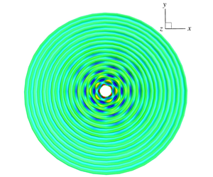
Contour snapshots of the surface wave fields from direct numerical simulations, which are radiated by vertical harmonic oscillations of a floating sphere (located at the centre of the domain). (a) Steady state base ring wave at $t_{1}/T_{0}=0$ ($2\unicode[STIX]{x1D714}_{0}=40\unicode[STIX]{x03C0}~\text{rad}~\text{s}^{-1}$, $k_{0}r_{1}=3.98$, $a/r_{1}=0.12$); (b) total disturbed wave field at $t_{1}/T_{0}=10$ (composed of base ring wave in (a) and initial subharmonic cross-wave disturbance with azimuthal wavenumber $m=5$ and free-surface slope at waterline $s_{0}=0.1$); (c) total disturbed wave field at $t_{1}/T_{0}=6$ (composed of ring wave with $2\unicode[STIX]{x1D714}_{0}=35\unicode[STIX]{x03C0}~\text{rad}~\text{s}^{-1}$ and $a/r_{1}=0.2$, and initial subharmonic cross-wave disturbance with $m=4$ and $s_{0}=0.1$); and (d) total disturbed wave field at $t_{1}/T_{0}=6$ (composed of ring wave with $2\unicode[STIX]{x1D714}_{0}=30\unicode[STIX]{x03C0}~\text{rad}~\text{s}^{-1}$ and $a/r_{1}=0.3$, and initial subharmonic cross-wave disturbance with $m=3$ and $s_{0}=0.1$).

8.1 Initial disturbance phase effect

To understand the effect of the phase of the initial distance upon the instability, we consider the initial cross-wave disturbance with an arbitrary initial phase $\unicode[STIX]{x1D6FA}_{0}$ with free-surface potential and elevation of the disturbance given by

(8.1)$$\begin{eqnarray}(k_{0}^{2}/\unicode[STIX]{x1D714}_{0})\overline{\unicode[STIX]{x1D719}}_{m}^{\prime }=\text{Re}(\overline{\unicode[STIX]{x1D711}}_{m}\text{e}^{-\text{i}\unicode[STIX]{x1D714}_{0}t}\text{e}^{\text{i}\unicode[STIX]{x1D6FA}_{0}});\quad k_{0}\overline{\unicode[STIX]{x1D701}}_{m}^{\prime }=\text{Re}(\overline{\unicode[STIX]{x1D702}}_{m}\text{e}^{-\text{i}\unicode[STIX]{x1D714}_{0}t}\text{e}^{\text{i}\unicode[STIX]{x1D6FA}_{0}}),\end{eqnarray}$$

where $\overline{\unicode[STIX]{x1D711}}_{m}(r,\unicode[STIX]{x1D714}_{0})$ and $\overline{\unicode[STIX]{x1D702}}_{m}(r,\unicode[STIX]{x1D714}_{0})$ are obtained from appendix C. At the initial time $t=0$, we add small cross-wave (with $m=5$) disturbances with $\unicode[STIX]{x1D6FA}_{0}=\unicode[STIX]{x03C0}/4$, $\unicode[STIX]{x03C0}/2$, $3\unicode[STIX]{x03C0}/4$ and $\unicode[STIX]{x03C0}$ to the ring wave field (with $2\unicode[STIX]{x1D714}_{0}=40\unicode[STIX]{x03C0}~\text{rad}~\text{s}^{-1}$ and $a/r_{1}=0.12$) to investigate the initial disturbance phase effect on the instability development. Figure 16 compares the time evolution of the growth rate $\unicode[STIX]{x1D706}_{51}(r=r_{1})$ of unstable subharmonic ($\unicode[STIX]{x1D714}_{0}$) component of azimuthal wavenumber $m=5$ for different $\unicode[STIX]{x1D6FA}_{0}$ values. It is seen that $\unicode[STIX]{x1D6FA}_{0}$ apparently influences the initial evolution of $\unicode[STIX]{x1D706}_{51}$, but does not alter its steady state value after the initial transient effect vanishes.

This phenomenon bears a resemblance to the ‘phase-locks’ in subharmonic resonance of a simple pendulum (Bogoliubonv & Mitropolsryy Reference Bogoliubonv and Mitropolsryy1961; Minorsky Reference Minorsky1974). In the pendulum case, both the amplitude and phase of the disturbance initially vary with time and depend on each other in a complicated way. The phase will eventually diminish/increase to the locked phase, and the amplitude will exponentially grow/decay with time. In the present case, the cross-wave’s locked phase is seen to be around $\unicode[STIX]{x1D6FA}_{0}=\unicode[STIX]{x03C0}/4$. The locked phase value, however, may depend on the base ring wave and disturbance cross-wave parameters.

Figure 16.

The time history of the growth rate $\unicode[STIX]{x1D706}_{51}$ of unstable subharmonic cross-wave ($m=5$) with different initial phases: $\unicode[STIX]{x1D6FA}_{0}=\unicode[STIX]{x03C0}/4$ (——), $\unicode[STIX]{x1D6FA}_{0}=\unicode[STIX]{x03C0}/2$ (– – –), $\unicode[STIX]{x1D6FA}_{0}=3\unicode[STIX]{x03C0}/4$ (— ⋅ —) and $\unicode[STIX]{x1D6FA}_{0}=\unicode[STIX]{x03C0}$ (— ⋅ ⋅ —). For the base ring wave, $2\unicode[STIX]{x1D714}_{0}=40\unicode[STIX]{x03C0}~\text{rad}~\text{s}^{-1}$, $k_{0}r_{1}=3.98$ and $a/r_{1}=0.12$.

8.2 Initial disturbance wavenumber (shape) effect

It is of interest to see whether the wavenumber (related to the spatial shape) of the initial disturbance influences the formation of unstable modes of the ring wave. To study this, we consider the base ring wave with $2\unicode[STIX]{x1D714}_{0}=40\unicode[STIX]{x03C0}~\text{rad}~\text{s}^{-1}$, $k_{0}r_{1}=3.98$ and $a/r_{1}=0.12$. The initial disturbance corresponding to cross-wave modes ($m=5$) with frequency $0.5\unicode[STIX]{x1D714}_{0}$, $2\unicode[STIX]{x1D714}_{0}$ and $3\unicode[STIX]{x1D714}_{0}$ is added into the base ring wave, separately. Figure 17 shows the time evolution of the harmonic amplitudes of disturbance elevation at $r=r_{1}$ (near the waterline) during the nonlinear evolution of the disturbed ring wave field, obtained with initial disturbances of a different shape. It can be seen that, even though the initial cross-wave disturbance possesses a different shape (wavenumber or frequency), the $\unicode[STIX]{x1D714}_{0}$ component (that is a subharmonic to the base ring wave) is always excited, due to the non-orthogonality of the $\unicode[STIX]{x1D714}_{0}$ cross-wave mode with all other modes of different frequencies, and grows exponentially with time, eventually becoming a significant component comparable to the base ring wave component in the wave field. This result indicates that the (unstable) subharmonic cross-waves will be predominantly developed in the ring wave field for any initial disturbance.

We remark that without the addition of initial seeded cross-wave perturbations, the small numerical noise in the simulation would also lead to the apparent development of sub-harmonic unstable modes, but with a much longer time of simulation due to the small amplitude of the numerical noise. To reduce the computational cost associated with the long-time simulation, in this work, we choose to add seeded perturbations (with their amplitudes much larger than the numerical noise) to examine the development of dominant unstable modes of the ring wave.

Figure 17.

The time history of the harmonic amplitudes of disturbance elevation near the waterline with the initial cross-wave ($m=5$) disturbance frequency equal to (a) $0.5\unicode[STIX]{x1D714}_{0}$, (b) $2\unicode[STIX]{x1D714}_{0}$ and (c) $3\unicode[STIX]{x1D714}_{0}$. For the base ring wave, $2\unicode[STIX]{x1D714}_{0}=40\unicode[STIX]{x03C0}~\text{rad}~\text{s}^{-1}$, $k_{0}r_{1}=3.98$ and $a/r_{1}=0.12$. The plotted curves represent the amplitudes of harmonic components with frequency equal to $0\unicode[STIX]{x1D714}_{0}$ ($\cdots \cdots$), $0.5\unicode[STIX]{x1D714}_{0}$ (—  —), $\unicode[STIX]{x1D714}_{0}$ (——), $2\unicode[STIX]{x1D714}_{0}$ (– – –), $3\unicode[STIX]{x1D714}_{0}$ (— ⋅ —) and $4\unicode[STIX]{x1D714}_{0}$ (— ⋅ ⋅ —).