1. Introduction

Recent years have seen a developing discussion on the role and epistemology of simulation in modern scientific practice, as a subject worthy of its own attention, distinct from experimentation and modeling. With some exceptions, particularly in the case of ecology and social science, most attention in the philosophy of science literature has been given to physics-based cases, such as meteorology, climate science, and nanoscience, where theories such as fluid dynamics and quantum mechanics provide essential material from which particular simulation models take shape. This article aims at a new contribution to this discussion, by looking at cases in which researchers build simulations without a theoretical starting point and without “theoretical articulation.” We focus on ethnographic studies of cases from the relatively nascent field of integrative (computational) systems biology (ISB), for which the principal product of investigation is a simulation.Footnote ¹ Systems biologists regard themselves as engaged in a genuinely new enterprise that cannot be subsumed within the bounds of established biological fields like molecular biology or physiology. They build computational models of the fluxes of material and information in complex genetic and metabolic networks. However, instead of articulating theories into informative computational models, systems biologists compose their models by collecting essential dynamical and structural information themselves from a variety of sources, including from their own simulations in highly iterative and intensely cognitive process (see also Chandrasekharan and Nersessian Reference Chandrasekharan and Nersessian2011).

This article has two principal aims. First, we illustrate with the help of a case study of one modeler’s PhD research how systems biologists, at least those in the bottom-up strand of systems biology (Bruggeman and Westerhoff Reference Bruggeman and Westerhoff2007), build their simulations from the “ground up,” by piecing together in a nest-like fashion principles from molecular biology, experimental results, literature surveys, canonical models, and computational algorithms to create representations of systems in data-poor environments. Such a study helps broaden our understanding of the range of scientific practices involved in the production of simulations. This is required if we want to attain a general perspective or understanding of what simulation is across a broader range of disciplines and also of the important roles of simulation for novel disciplines that have come into being because of computer technology, for which simulation is the central defining methodology (see also Lenhard Reference Lenhard2007).

Second, in light of a developing discussion about the role of theory in modern computationally and data-driven biology (see, e.g., Leonelli Reference Leonelli2012a, Reference Leonelli2012b), we use this case study and broader opinions from within the field to reflect more broadly on the different meanings and functions of “theory” in systems biology, particularly with respect to attempts to establish mathematical templates for the field. More generally, systems biology aims to invert the dictum that theory produces or facilitates simulation. It is the rhetoric of systems biology that a theory of biological systems will emerge from model building and simulation.

2. What Do We Know about Simulation in Science?

We already have some good philosophical analysis of the role of simulation in various scientific contexts. For instance, Humphreys, Lenhard, Winsberg, and Parker have detailed the importance of simulation to the success of various fields like nanoscience, shock wave theory, and meteorological and climate models, by applying theories of structure and dynamics from quantum mechanics and fluid dynamics to complex phenomena (see Winsberg Reference Winsberg1999, Reference Winsberg2001, Reference Winsberg2003, Reference Winsberg2009, Reference Winsberg2010; Humphreys Reference Humphreys2002, Reference Humphreys2004; Lenhard Reference Lenhard2006, Reference Lenhard2007; Parker Reference Parker2006, Reference Parker2010a, Reference Parker2010b). They have discussed particularly the various epistemic roles simulation plays in comparison with ordinary model building and also with experimentation. Both Lenhard and Winsberg claim strongly that simulation brings a unique methodology to scientific practice that requires its own epistemic principles. Simulations, for instance, necessarily require that a model be transformed into computational language that imposes its own constraints such as computational speed and memory capacity and requires its own unique decision-making principles such as those for discretizing continuous differential equations. Such principles, Winsberg (Reference Winsberg1999, Reference Winsberg2010) contends, are not given by theory. He describes simulations, rather, as “semiautonomous” of theories, by which he means that although one starts from a theory, “one modifies it with extensive approximations, idealizations, falsifications, auxiliary information, and the blood, sweat, and tears of much trial and error” (Reference Winsberg2003, 109).

Winsberg further points out that simulation models are often generated because data are sparse. Simulations step in to provide a source of data and, thus, a way of exploring a phenomenon for which experimental access is otherwise limited. Lenhard (Reference Lenhard2007) in turn has emphasized the role simulation experiments play in exploring the consequences of a theoretical model, through a process he calls “explorative cooperation.” This invokes many extratheoretical techniques that allow a theory and its models to be articulated to fit the phenomena. Such explorations are largely driven “from above” by the data and fitting the data, not by the theory. Lenhard (Reference Lenhard2006), with help from Humphreys (Reference Humphreys2004), has also argued that simulation is effecting a change in deeper aspects of the epistemology of science. In some cases, a model built out of a particular theory acts in an “epistemically opaque” way, meaning the theory cannot be used to produce an understanding of a phenomenon by, for instance, analytically solving the equations. The theoretical model developed from a theory is so complex that the only way to discover its consequences is through simulation. Hence, simulation provides a resource for exploring complex phenomena through the dynamics of a model. As such, a kind of law-based or even mechanistic understanding cannot be had. Instead, researchers produce a pragmatic level of understanding through their ability to control and manipulate a phenomenon through simulation.

Along a different but related line, Parker has been grappling with how climate science and meteorology researchers, while relying on available physical theory in building simulation models, handle the indecisiveness or indeterminancy of this theory for pinning down the best representational strategies of the many it makes available (Parker Reference Parker2006, Reference Parker2010a, Reference Parker2010b). Theory in these fields offers a model-building framework but no way of evaluating easily the best of the alternative models that can be built using this framework, given available data. These researchers grapple with the resulting uncertainty, by collectively employing multiple models making different, sometimes conflicting, structural and parametric assumptions and approximations in order to bootstrap climate and weather predictions. These ensembles are thus particular strategic responses to the inadequacy of theory. However, Parker questions strongly whether such a strategy can justify its predictions without recourse to a theory that can determine whether an ensemble adequately represents the space of possibilities.

We think many of the philosophical insights about simulation apply in the case of systems biology and have genuine claim to descriptive generality across scientific fields that employ simulation. Simulation must be approached on its own terms and cannot be reduced to modeling or experimental practices. We think, however, that there needs to be more discussion of the roles theory and theoretical models play in the production of simulations. For the most part, the central concern of both Lenhard and Winsberg, following earlier work with modeling in general (see Savageau Reference Savageau1969b; Morgan and Morrison Reference Morgan and Morrison1999), has been to demonstrate how simulation is autonomous or semiautonomous from background theory, by elaborating the extratheoretical factors that contribute to simulation production. These are usually justified by how well they produce simulations that match the phenomena, not by their accordance with theory. Winsberg (Reference Winsberg1999, 277) admits himself, however, that his conclusions about simulation do not necessarily apply in cases in which theory does not play an explicit part.

However, a collection of researchers studying modeling in ecology and economics have begun to attend to how simulations in these fields come to be constructed often without any process of theoretical articulation. Instead, simulations in these fields rely on diverse methodologies and nonstandardized techniques tailored to the specific problems at hand (Peck Reference Peck2008). These observations are reflected in the increasing reliance on agent-based modeling in ecology (Peck Reference Peck2012). Agent-based modeling simulations rarely start from a systematic theory “because of the difficulty of finding general ecological theories that apply across a wide range of organisms and the deeper suspicion that we do not have any in the same sense as models found in the physical sciences” (5). Agent-based models provide a means for modeling without theoretical knowledge because “we usually do know something about agential behavior through data” (5). Ecologists themselves are grappling with how to standardize the resulting eclectic mix of practices and descriptions that characterize agent-based models that lack the communicability and analyzability of traditional analytic models (Grimm et al. Reference Grimm, Berger, Bastiansen, Eliassen, Ginot, Giske, Goss-Custard, Grand, Heinz and Huse2006, Reference Grimm, Berger, DeAngelis, Polhill, Giske and Railsback2010). We think the same applies to systems biology, where the models also do not admit of analytic solutions and simulation is necessary, although in this case the models for the most part are ordinary differential equations (ODEs) rather than agent based.

Our aim here is to advance the discussion of how simulation models are constructed without recourse to a body of theory that provides the structure and dynamics of the phenomena under investigation, through drawing on our ethnographic analysis investigating the fine details of ISB model-building processes and the cognitive affordances of those processes. Nor is there a generally accepted theory applying across the domain of such systems that specifies the routines and formalisms that can and should be followed and applied to model such systems. The responses the participants in our study make to the lack of theory that they can articulate into models of their systems, as well as to limited data and the complexity of the subject matter, are no doubt shared with other fields, like ecology, in which modelers find themselves in similar situations. Thus, this case study should have broader relevance for a philosophical understanding of simulation model-building practices across a range of modern simulation-driven scientific contexts. Our first task, however, is to come to some terms with what systems biology is and how it works.

3. What Is Integrative Systems Biology?

In principle ISB is relevant to any biological systems from ecological systems to genes, although in practice, and certainly in the labs we study, most research is directed at cellular or intracellular systems. As such, systems biology presents itself as new approach to understanding and controlling systems like gene regulatory or metabolic networks through computer simulations of large-scale mathematical models. It applies computer technology to what was formerly considered inaccessible complexity, in order to generate representations of the dynamics of these networks, particularly material and informational fluxes through a network of cells or biomolecules. Importantly, systems biologists claim they are working to understand the system-level properties of a network or the dynamic patterns of a network, rather than pulling apart the details of the interactions of its components. In Kitano’s terms, a diagram of gene and protein interactions provides insight on how a system works, “it is like a road map where we wish to understand traffic patterns and their dynamics” (Reference Kitano2002, 2). Systems biologists contrast this approach with traditional molecular biology that pursues these elements such as gene and protein interactions “in isolation,” that is, through in vitro analyses of the properties and structure of individual biomolecules. ISB studies these molecules in their systemic contexts as part of a functioning unit.

ISB is not, however, a homogenous enterprise, as we have discovered in our own investigations. Researchers in the field and philosophers identify two broad strands, namely, top-down and bottom-up systems biology (see Bruggeman and Westerhoff Reference Bruggeman and Westerhoff2007; Krohs and Callebaut Reference Krohs, Callebaut, Boogerd, Bruggeman, Hofmeyr and Westerhoff2007). Top down relies on high-throughput technology that takes repeated simultaneous measurement of large numbers of chemical concentrations within cells, enabling a great quantity of time-series data for many cellular elements to be collected. Computer methods can then be used to “reverse engineer” system structure by sorting through correlations in those elements. Bottom-up systems biology, however, “reproduces” (or simulates) systems with dynamic models, by drawing on knowledge of network structure and the kinetic and physicochemical properties of its components. Its data tend to come from molecular biology sources.

Our investigations principally concern bottom-up systems biology. Since such metabolic and genetic systems are generally extremely complex cases of continuous nonlinear systems, computer technology is required not only to run the dynamic models but also to provide the power to graph their dynamics (highly important for understanding networks), estimate parameters and parameter sensitivities, and calculate steady states and analytic network measures like flux control coefficients. Since much of bottom-up systems biology works in relatively data-poor environments, algorithmic techniques of evaluating networks for their solvability and estimating parameters is a computationally intensive process. One of the ultimate aims is to be able to gain sufficient fine-tuned control and understanding of the input and outputs of a biological network to be able to manipulate it to produce desired outcomes, such as increased production of a good chemical (e.g., a biofuel) or reduction of bad one (e.g., a cancer-causing agent).

Systems biologists in the labs we have been studying fit, for the most part, within the bottom-up tradition, although with distinct methodological differences in the ways the labs work (MacLeod and Nersessian 2013;Nersessian and Newstetter Reference Nersessian, Newstetter, Johri and Olds2014). One thing they do share is that most researchers come almost uniformly from engineering rather than biological backgrounds and bring metaphors and analogies such as electrical circuit analogies and concepts like noise, control, robustness, redundancy, modularity, and information with them to understanding biological systems. The heavy systems engineering and control theoretical perspective is very important to piecing together the thought processes driving systems biology in practice, particularly the belief that system-level understanding is not contingent on a detailed theory of the mechanical interaction of network components. It is more fairly described as “mesoscopic” or “mesoscale” or “middle-out modeling,” rather than bottom up (see also Westerhoff and Kell Reference Westerhoff, Kell, Boogerd, Bruggeman, Hofmeyr and Westerhoff2007; Voit, Qi, and Kikuchi Reference Voit, Qi and Kikuchi2012). Mesoscale modeling works on the basis that nonlinear and complex system dynamics are emergent properties of network structures that do not require detailed lower-level theory (whether physics, biochemistry, or molecular biology) to reconstruct and understand.

4. Building from the Ground Up

In simulations derived from theory, particularly physical theory, the modeling process starts with the theory, or at least with a theoretical model that traces its origins to a theory. Of course “theory” is a contested and multifarious category, and we do not mean to use it uncritically. What we are referring to here is a broad eclectic understanding of theory as a reservoir of laws, canonical theoretical models, principles of representation (such as boundary conditions), and ontological posits about the composition of phenomena that guide, constrain, and resource the construction of models in diverse disciplines across a wide spectrum of physical systems. From Cartwright (Reference Cartwright1983) on, a number of philosophers have claimed that we need to be circumspect about the role theory plays in physics and physics-dependent disciplines, and it cannot be said in any sense that models are simply derived from theories (see, e.g., Morgan and Morrison Reference Morgan and Morrison1999). We start from the view, nonetheless, that in these physics-based fields theory is playing some role, and this role is essential, even if it is not as strong as we might have once presumed. Mesoscopic modeling, however, starts without such a reservoir of fundamental models, laws, and principles.

Our investigations take the form of a 4-year ethnographic study of two biochemical systems biology laboratories. One lab (“Lab G”) models only in collaboration with experimental researchers outside the lab.Footnote ² The other lab (“Lab C”) conducts its own experiments in the course of building models. The labs are populated largely by graduate students. We use ethnographic data-collection methods of participant observation, informant interviewing, and artifact collection. In both labs, we conducted unstructured interviews with the lab members and some collaborators outside of the lab. We collected and analyzed relevant artifacts including Powerpoint presentations, paper drafts, published papers, grant proposals, dissertation proposals, and completed dissertations. Thus far, we have collected 97 interviews and tape-recorded 24 research meetings. From these investigations, we have built up a detailed understanding of how simulations are constructed by the researchers (Chandrasekharan and Nersessian Reference Chandrasekharan and Nersessian2011; MacLeod and Nersessian Reference MacLeod and Nersessian2013). We think their practice can suitably be described as modeling from the ground up.Footnote ³ By modeling from the ground up, we identify a pair of entwined modeling practices. First, modelers assemble the structure and local dynamics of the phenomena being modeled largely from scratch (and not from a theoretical starting point), by pulling in empirical information from a variety of sources and piecing it together into an effective representation by using a variety of assumptions and simplifications and mathematical and computational techniques. Every part of this process is open to choice about the methods to use and the information to include. Second, modelers rely cognitively on the iterative building process and their preliminary simulations, to understand their systems and adapt their representations of them to their particular epistemic goals. This feature signals the more intensive role simulation and model building have as cognitive and epistemic resources in the context of a modern computer-driven discipline.

5. Case Study: G12 and Atherosclerosis

To flesh out our ideas, we have chosen as an exemplar one of the graduate researchers we followed from Lab G. We refer to her as G12. Her experiences and model-building practices are strongly representative of the practices of the other modelers we have tracked across both labs. As her research unfolded, G12 gave us detailed descriptions of the processes by which she put together her models, demonstrating the ways in which our ISB researchers assemble their models from the ground up in a nest-like fashion. That is, just as a bird will gather almost anything available to make a stable nest, G12 pulled together and integrated bits of biological data and theory, mathematical and computational theory, and engineering principles, from a range of sources, in order to generate stable robust simulations of biological networks. This was an intensely constructive process that lacked a coherent theoretical resource as a basic platform from which she could work. Instead, she had to bring together and integrate whatever techniques and information were available and continually adapt and adjust her own representation of her systems within the affordances and constraints of these techniques. Our reconstruction of her model-building process arranges it into three segments, but this should be understood as only approximate since, in fact, model building is not a linear process.

Her ostensible research topic was the relation between oxidative stress and the generation of monocytes implicated in the generation of plaques on the vascular smooth muscle cells of blood vessel walls. Such activity is thought the main cause of conditions like hypertension and atherosclerosis, which result from the hardening of arteries and loss of elasticity caused by these plaques. G12 produced three models in completing her PhD research covering different aspects of this problem in different cell lines (table 1). Like virtually all of the student researchers in both of these labs, G12’s background is in engineering, not in biology. In terms of the biology, she always felt that she started “from zero” with every new modeling task on a different biological system. Indeed the model-building process is a way through which Lab G researchers learn the relevant biology. G12’s process was built around three main interrelated tasks. First, the construction of a biological pathway; second, the construction of a mathematical representation of that pathway; and third, an estimation of parameters for the mathematical representation that would fit it to the dynamics observed in experiment.

Table 1.Description of G12’s Models

	Description
Model 1	Pathway in endothelial cells through which particular mechanosensitive genes produce oxidative stress in response to different vascular fluid stresses
Model 2	Assembly and disassembly mechanism in smooth muscle cells of an enzyme critical in redox cycling and oxidative stress
Model 3	Pathway by which a hormone A produces oxidative stress in smooth muscle cells

5.1. Constructing the Pathway

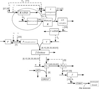
In each case, G12 had to begin by putting together a pathway of the molecular interactions and signaling relations composing the biological network. In each case, the pathway given to her by her collaborators was insufficient given her modeling goals, and she was forced to pull in whatever pieces of information she could find from literature searches and databases about similar systems or the molecules involved, in order to generate a pathway that mapped the dominant dynamic elements. For example, in the case of her first pathway diagram for model 1, she was given a pathway by her experimental collaborator but quickly realized this pathway would not be adequate in itself to produce a model that could explain the dynamics of the relationship between her mechanosensitive gene X and reductive oxygen species production. G12 stated, “Yeah so actually first I read the literatures and I find, I need to know even though he gave me the pathway, I need to know whether there are any other contributing factors, whether there are other important factors that are missing.”

The focus of her collaborator on this project, as a molecular biologist, had been on assembling the main direct chain of causal influence, not on what other contributing factors would be affecting the system’s dynamic behavior, which was necessary for G12’s task. Reading through her collaborator’s and other literature, G12 began to “figure out” and pull together what other factors and interactions were involved and thus produce a more comprehensive pathway. Starting out with only five variables, the final production had expanded to 14. As she put it, “but um he didn’t say clearly how the things interact. Even in the, this diagram (Figure 1), there’s something missing. There are missing steps I combine them together because I don’t know how exactly this upstream one affect the downstream one. So in his papers there are several things I connect them together, and I need to make sure … how from this, the upper one goes to the downstream. So I need to go verify.”

Verification in this context means either checking the literature or asking her collaborator. At some point running preliminary simulations, she noticed that there needed to be another component that was not accounted for in the literature she had on the system, in the form of signaling between X mRNA and the X precursor (circled in fig. 1). She inserted this signaling relation because she had inferred the potential interaction from reading about X and its properties. This addition was made without explicit experimental evidence for its role in this system.

Figure 1.

Pathway diagram used by G12 in the construction of model 1. The chemical names of the reactants have been substituted by us. The two mechanically different types of stress applied to the system are S1 and S2. Numbers in brackets refer to the specific references from the literature used in building out the pathway. Solid lines indicate material flow through the pathway, while dashed lines indicate signaling without the flow of material, and indicates time delay. The circled relation between X mRNA and X precursor G12 hypothesized herself.

Building these pathways was not simply a passive process of recording information. It involved significant effort on her part to produce pathways that were sufficient to reproduce the dominant network dynamics while staying within the data constraints and without the network representation becoming too complex for parameter estimation. In this first model, particular simplifications and assumptions were applied in order to be able to represent the system as simply as possible, so that her mathematical frameworks and parameter estimation techniques could handle the lack of good data on the system. This is a common type of accommodation our modelers bring in. It included only considering two elements of the Z oxidation system, the protein P and enzyme Y, by assuming on the basis of information in the literature that other elements did not interact with X and probably did not strongly affect the pathway. The model 1 pathway in the final result, thus, tracked for G12 the dominant interactions that occur from the introduction of two mechanically different types of stress (S1 or S2) to the production of excess-plaque-inducing monocytes.

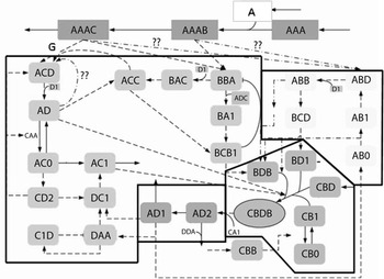
Model 2 was an attempt to construct a pathway lacking in the literature for the activation of an enzyme CBDB that would be critical for model 3. This network is built into her pathway diagram for model 3 as the module of the bottom-right corner (see fig. 2). In the interest of space, we just focus here on model 3. In building the pathway for model 3, she brought a range of techniques to bear. Here, G12 aimed to model the role of hormone A, rather than fluid stress (model 1), in the generation of oxidative stress and inflammation.

Figure 2.

Preliminary pathway diagram for model 3. Metabolite names have been replaced. G12 color coded her modularization of the network, which we have marked off with boxes. The top-left box is the BCB1 module, the top right is the AB0/AB1/ABD signaling cascade system, the bottom right is the CBDB activation system (model 2), and the last middle-bottom box represents the reduction oxidation module. This is not the completed diagram but represents a stage in G12’s work. Particular unknowns are represented with ‘??’.

G12 built this pathway as her own simplified representation, “having collected and interpreted all related information from literature as well as having consulted our experimental collaborators.” The pathway was broken up into manageable modules, designated in figure 2. Constructing this complex pathway required pulling together bits and pieces of information and a full variety of techniques, ranging from offlining variables and blackboxing systems to informed guesses. She discovered the role of CB1 from the literature. In a major reconstruction, after running her first simulations, her collaborator told her of the importance of BDB, which G12 did not know about. This had to be added and the pathway adjusted.

In the case of the redox buffering system operating in this model (the module AD1/AD2 in fig. 2), she had blackboxed many of the components (components she was aware of from another researcher in a neighboring lab), particularly the systems of degradation for AD1, because of their complexity but also because the data she had were too poor to account for the elements of these systems: “I don’t want to separate them because it’s so complicated and then you don’t know the real concentration or the real molecule numbers.” Instead, G12 gave the buffer the system capacities she deemed necessary, by imposing, for instance, constant degradation rates.

Second, she made calculated decisions about offlining variables in the model and thus treating them as controlled inputs (rather than system-embedded variables). “Offlining” involves decoupling a variable from the dynamics of the system, because of a lack of information about how it connected to the system or because of the complexity of connecting it into the system, and instead feeding in its values by hand in order to get the model to fit the data. She expressed a plan to do this for a particular enzyme G: “So I just decouple, okay, I don’t have this, if uh, I would just input this and input have this effect on this enzymes and I would just input this, the effect of the enzyme directly.” She would either take the value to input from the literature or guess and experiment with the model.

G12 also had to apply her own limited biological knowledge, sometimes in contradiction to what the literature was suggesting, in order to limit her model. For instance, she had originally accepted the idea that protein BDB should be being recycled: that is, BDB would at some point dissociate, and its component antecedents like BCB1 would reemerge (see fig. 2). Overall, the number of proteins would not change at the basal level, which was stable. She thought, however, that this would involve continuous translocations of the components from across the cytosol and plasma membrane and back, which made her uncomfortable because it seemed to be invoking too many assumptions she could not justify. “So before I use recycling assumption in something like this but right now I think probably it’s not appropriate, I don’t know why, just a feeling.” Instead, it seemed reasonable to her to just have the protein degrade at a certain rate, balanced by the rate of incoming components.

In each case, these pathway representations were composed from a variety of sources and with a variety of techniques. G12 built in information that emerged in the process of building dynamic models of the pathways, but she also controlled the pathway representations through different techniques to restrict these representations to what could be modeled manageably and reliably.

5.2. Mathematical Frameworks and Mathematical Simplifications

G12 also had to decide what kind of formalisms to use to model the data. This decision for systems biologists ranges over the very fundamental choices of whether to use phenomenal models like agent-based models or mechanistic models, discrete or continuous models, spatial (partial differential equation) versus nonspatial (ODE) models, stochastic or deterministic models, and multiscale or uniscale models. In our labs, they almost all decide to try to put together an ODE system, given its relative conceptual simplicity and potential informativeness as well as the range of computational and mathematical infrastructure that exists for estimating parameters and analyzing model dynamics. Choosing an ODE framework opens up another range of very important choices over whether, for instance, to model the system as at steady state (static) or away from any equilibrium and whether to use a straightforward mass-action/stoichiometric model, a mathematical template like biochemical systems theory (BST; see the next section) that tends to build in or average over the details of interactions, or a mechanistic model that builds in equations closer to the molecular biological details in the form of rate laws of individual enzymatic interactions such as Michaelis-Menten or ordered uni-bi mechanisms. Such decisions are made as part of a calculated integration of a wide variety of constraints that modelers have. Certainly no modeling strategy is universally the best or most accurate under all circumstances. It depends both on the objective the researcher has and certainly on the completeness and the nature of the data she has.

In G12’s case, she oscillated between the use of mass action models and BST, in the form of generalized mass action (GMA) models (which use power law representations of interactions). For her first model, few dynamic data were available. Most were qualitative, in the form of observations from experiments that x up or down regulates y. At the same time, the model involved multiple timescales since it involved genetic transcription, protein transcription, and enzyme-catalyzed biochemical reactions. This meant that she needed a framework in which time delays could be easily incorporated.

For these tasks, the GMA framework was appropriate. This framework models the system as ODEs, modeling flux as the sum of inputs minus outputs:

Its prime attractive property in these circumstances is that it can account for a large variety of dynamics, by modeling the flux of dependent variables as power laws. This means that even if the nature of interactions between elements is not well known for the system, there is a good chance that the system dynamics will still be accounted for within the range of realistic parameters for the system. In G12’s second model (model 2), however, the actual quantitative dynamic data on the system (as opposed to its composition) were extremely limited, so she had to fashion her aims and the model to meet this constraint. In this case, because the pathway was well drawn up in most details, a simple mass-action model sufficed and would invoke fewer unknown parameters. Second, because the critical enzyme CBDB (see fig. 2, pathway for model 3) mostly operated in a basal condition of steady state in the body, she could derive the structural features she was looking for at steady state. From steady state, she was able to derive a set of linear relationships between fluxes and then analyze them according to various optimization conditions, namely, what would produce the maximum responsiveness in the least time to any stimulation of the system out of the basal condition. Hence in this case, in addition to bringing in a particular mathematical framework to help her construct a representation, G12 also added certain mathematical simplification techniques to transform her problem into one she could handle with such limited data. As mentioned, the information from model 2 about CBDB activation was used to help construct that module in model 3, on the assumption that the steady state–derived structure and parameters would hold too in the dynamic context of the system undergoing stress.

6. Theory in Systems Biology

Although we have examined how the systems biologists in our labs work without the reservoir of essential information about their systems that physical theory would provide on how to build models in a domain, we do not mean to be arguing that concepts of theory have no currency within ISB. As has been long understood by philosophers, “theory” has diverse connotations in practice. Systems biologists use “theory” to refer to a plethora of different bits and pieces of information from, for example, molecular biology and mathematics, which they pull together to build their simulations.

However, one of the principal elements of simulation building that goes by the name “theory” in the context of systems biology are “canonical” ODE models. An example is BST, which is used at times by Lab G participants to model their systems and comes with a collection of analytic tools.Footnote ⁴ BST posits that the processes of a given metabolic/signaling network can be modeled dynamically as power law functions. There are two types of canonical representation, GMA and S-System formats. First, GMA uses ODEs of this type:

where is the number of terms in the ith equation. The ’s represent the concentrations of the various molecular elements in the network. Each separate flux in and out is represented by an individual power law.

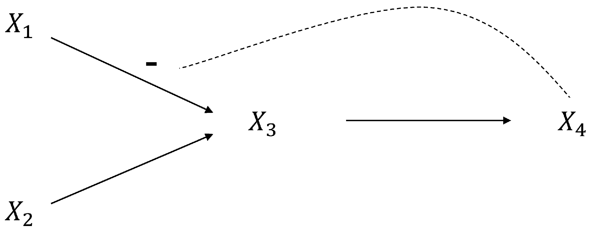
For example, in the case of the system in figure 3, we model as

The S-system format, however, pools all the effects of ingoing and outgoing flux into one separate term:

In this case,

Applying these canonical models is a matter of filling in the network details (which ’s are interacting with which others), the parameters with which such interactions take place (the kinetic orders h, g, and f’s), and the rate constants (the , , ’s). Canonical templates fit with Humphreys’s concept of a computational template (Reference Humphreys2004). These templates are not constructed from theoretical templates or laws, however, a case Humphreys acknowledges as perfectly possible with the example of the Poisson process (88). We think the case of BST illustrates how computational templates get used and constructed differently in different fields, particularly when compared to canonical cases in the physical sciences. The most important point is that BST and its templates are not starting points of the modeling process, in the way a theoretical template or theory often is in the physical sciences. They are chosen, if suitable, during the model-building process (as we have shown in the case study) and modified as required. The framework, in other words, is added to the nest in the model-building process, if it serves that process given the available data and the aims of the modeler. This usage identifies a different role that these templates play in simulation building, which in turn signals a difference of intent of a theory like BST.

Figure 3.

Sample metabolic network with feedback signaling.

Principally, rather than providing essential structural and dynamical information about a system out of which a simulation can be built through approximation and simplification, BST provides a schema of approximation and simplification for organizing effectively the information that a systems biologist has assembled. As such, BST offers a theory of how to model effectively and efficiently the dominant dynamics of complex biological systems in which data are sparse and systems complex. It instructs systems biologists how to average over (or linearize) the complexities of the mechanisms that govern the interaction between elements, in order to robustly match the dominant or key dynamic relationships in a network. The power laws above like are just such averaging relations. They are motivated by sound mathematical principles of approximation theory (first-order Taylor series approximations), given the biological assumption that the range of variation of concentrations of biological molecules is generally limited. BST assumes that, for most biological metabolic and signaling networks, suitable parameters can be found that will model to a high degree of accuracy the complex fluxes of the networks because the BST framework is flexible enough to capture them within the range of suitable parameter choices. In terms of efficiency, power law representations are telescopic. Power laws can be used generally to represent lower levels, and S-systems keep their structure when variables are substituted for lower-level systems. Further, such systems are readily analyzable mathematically, and system parameters can be clearly mapped to experimental measurements (Voit Reference Voit2000).

In contrast then to the role of theory in physics-based modeling, a theory like BST does not provide essential structural or dynamical information for describing the system. Dynamic fluid laws, for instance, contain essential information about the laws that govern the interactions of elements of mass or flux in a fluid system. In ISB the pathway and the nature of interactions have to be assembled by the researcher through the techniques and practices mentioned above, although once such templates are chosen they become routinely part of the cognitive systems researchers employ for exploring and revising their understanding of the biological system and for deciding how to approximate its structure and dynamics so as to provide the best model for their given aims. Each canonical model has its own advantages and disadvantages and domains over which it functions well. Power law models are more accurate than lin-log models for small substrate concentrations but not at high substrate concentrations. However, as (Voit Reference Voit2013, 106) points out, in practice the choice of canonical model is less important than “the connectivity and regulatory structure of the model.”

As a result, one cannot describe the fixing of parameters for these canonical models as a process of “theory articulation,” as it is described in physics-based contexts (see Winsberg Reference Winsberg1999, Reference Winsberg2003). The issue for systems biologists is not how to apply a particular background theory to a specific problem by adapting theoretical principles to the circumstances. Their project is to build a higher-level or system-level representation out of the lower-level information they have. Canonical templates mediate this process by providing a possible structure for gluing together this lower-level information.

This use of computational and mathematical templates is in fact at the heart of the philosophies and aims of ISB, which rejects an overly reductionistic approach to model building. As mentioned above, rather than bottom-up modeling, what systems biologists do can often be better described as mesoscale or middle-out modeling. Mesoscale models are “models of an intermediate size that are neither purely empirical nor contain complete mechanistic detail” (Nature Publishing Group 2011). These models try to ignore the complexities at the lower level, in order to capture the general features of a system’s dynamics and thus gain generic control over the network by mapping its important input and output relations. As Voit puts it, “All interactions must follow the laws of physics and chemistry, but accounting for every physical and chemical detail in the system would quite obviously be impossible—and is also often unnecessary. Canonical modeling provides a compromise between general applicability and simplicity that circumvents some of these problems by using mathematically rigorous and convenient approximations” (Reference Voit2013, 99). This creates an epistemology that favors techniques that average over the complex mechanisms at work at lower levels and provides ways to build functional models not just with sparse data but also with more manageable complexity as we saw with G12. Considered in this light, systems biology inverts the familiar relationship whereby theory contributes to models that in turn produce simulations. In ISB it is simulations, according to its promoters, that are being used to build up theory, although such theory is again not necessarily the same thing as theory in physics. Major figures in systems biology like Kitano (Reference Kitano2002) and Westerhoff and Kell (Reference Westerhoff, Kell, Boogerd, Bruggeman, Hofmeyr and Westerhoff2007) have been keen to emphasize the new promise of biological theory that the computational study of biological systems brings.

“The goal of systems biology is to offer a comprehensive and consistent body of knowledge of biological systems tightly grounded on the molecular level, thus enabling us to fully integrate biological systems into more fundamental principles” (Kitano Reference Kitano2002, 2). As Kitano points out, however, this does not mean we should expect something equivalent to fundamental laws. He prefers the example of theories like Bardeen, Cooper, and Schrieffer theory (the Cooper pairs theory), which explains superconductivity. Such a theory imposes its own specific constraints on a background of fundamental physical principles. Kitano sees systems biology similarly as discovering the structural constraints on the interactions of molecules, governed as they are by chemistry and physics. These constraints are often referred to as design and operating principles: particular structural features of networks that exemplify general evolutionary solutions to biological principles. These cross species’ lines. Design principles should help explain why nature “has settled on” some methods of building and running networks rather than others and thus, ultimately, compose a “biological theory.”

7. Conclusion

The philosophy of science has long discussed and explored the relationships between theory and models, a discussion that has now been extended to the relationship of theory and models to simulation. This discussion of modeling and simulation, however, remains incomplete. New computational sciences are breaking with the traditional patterns of model-building activity philosophers have typically observed. Ideas from engineering, mathematics, and computation and new large-scale data-collecting methods are being combined with biology to generate new interdisciplinary and transdisciplinary computational biological fields. In one such field, namely, integrative systems biology, we have detailed a practice of model building from the ground up, which builds simulation models without a theoretical starting point. These practices assemble a wide variety of resources together from different sources and leverage on the cognitive affordances of this incremental, nest-building process and simulation itself, in order to develop an understanding of a complex system’s dynamics and ultimately provide an adequate representation. As such, systems biology raises new issues about the role of theory in model building and epistemic issues about how understanding and credibility can be generated without a theoretical base.