Introduction
The human visual system can use various cues to segment a moving object from its surroundings. One strong cue, whether separate local motion signals originate from the same object, is the color and the contrast polarity of the local motion signals. At the early stages of motion processing, opposite contrast polarities are processed separately (Wehrhahn & Rapf, Reference Wehrhahn and Rapf1992; Westheimer, Reference Westheimer2007). With respect to motion integration, studies on the role of contrast polarity in combining local motion signals have focused on conditions where polarity and motion direction was correlated (Edwards & Badcock, Reference Edwards and Badcock1994; Croner & Albright, Reference Croner and Albright1997; Snowden & Edmunds, Reference Snowden and Edmunds1999; Li & Kingdom, Reference Li and Kingdom2001; Martinovic et al., Reference Martinovic, Meyer, Mueller and Wuerger2009;Cropper & Wuerger, Reference Cropper and Wuerger2005). In Croner and Albright (Reference Croner and Albright1997), a hue cue (only 10% of dots were of the same hue) was present that created a pop-out effect in the static display; when this static cue was removed (Snowden & Edmunds, Reference Snowden and Edmunds1999; Li & Kingdom, Reference Li and Kingdom2001), results were consistent with separate processing of local increments and decrements. The present experiment differs from these studies by employing stochastic motion stimuli in which the polarity and the motion direction is uncorrelated and therefore not providing redundant information about global motion.
For luminance-defined polarity differences (light/dark), the motion integration performance depends on spatial factors, and two competing integration mechanisms (ON/OFF) seem to be at work: same-polarity local motion signals are pooled within regions of a limited size, after which these ON and OFF mechanisms might be competing with each other (van der Smagt et al., Reference van der Smagt, Breij and van de Grind2000). These two mechanisms, that is, integration versus differentiation of local motion signals, may serve different functions in the segmentation of dynamic visual scenes (Braddick, Reference Braddick1993): competition between ON and OFF pools might arise due to the mechanisms that underlie transparency and figure-ground segmentation, whereas pooling over a large area containing local motion signals will increase motion sensitivity.
While there is convincing evidence that both ON and OFF motion pathways are mediating motion integration and segmentation in luminance-defined stimuli, much less is known about the role of contrast polarity for chromatic motion processing. The question remains whether the chromatic ON and OFF pathways are utilized for global motion processing in a similar fashion to luminance ON and OFF pathways. Therefore, our aim was to explore the role of contrast polarity for chromatic global motion processing. We utilized random dot kinematograms (RDKs) to gauge the effect of contrast polarity along two chromatic directions (L–M and S; see Fig. 1). In experiment 1, all dots were of the same contrast polarity (i.e., +LM, −LM, +S, or −S); in experiment 2, half the dots had a positive contrast polarity (i.e., +LM or +S); the other half had a negative contrast polarity (i.e., −LM or −S). By comparing the motion discrimination thresholds for the same-polarity and the different-polarity RDKs, we tested whether motion integration is selective for chromatic polarity.
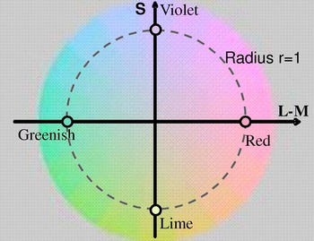
An isoluminant plane in DKL space is shown. Along the horizontal axis, the L–M-cone signals vary while keeping the sum constant. Along the vertical axis, only the S-cone signal is modulated. Stimuli were defined by a positive L–M- or S-cone signal (increments) or a negative L–M- or S-cone signal (decrements).

Methods
Apparatus
Experiments were run on a standard PC (Optiplex) controlling a ViSaGe system (Cambridge Research Systems Ltd., Kent, UK). The stimulus presentation was controlled by Matlab 2008 (Mathworks, Natick, MA), and the stimuli were presented on a 21-inch CRT monitor (SONY GDM-F520, Berkshire, UK) run at a refresh rate of 120 Hz. The chromatic and luminance output of the monitor were calibrated with a spectroradiometer (Photo Research PR650; Glen Spectra Ltd., Middlesex, UK). The monitor had been switched on for at least 30 min before the start of each experimental session. Observers were seated 50 cm from the screen in an otherwise dark sound-attenuated cubicle. The methods are described in more detail in previous papers (Ruppertsberg et al., Reference Ruppertsberg, Wuerger and Bertamini2003, Reference Ruppertsberg, Wuerger and Bertamini2007; Martinovic et al., Reference Martinovic, Meyer, Mueller and Wuerger2009). All eight participants had normal or corrected-to-normal vision. We tested participants’ color vision with the Cambridge Color Test (Regan et al., Reference Regan, Reffin and Mollon1994). Participants were informed about the objective of the study and they gave their signed consent. Experimental procedures were in accordance with the British Psychological Society guidelines on experimentation with human observers and have been approved by the University of Liverpool Ethics Committee.
Stimuli
We used sparse RDKs with 50, 100, or 200 colored Gaussian blobs, varying either along the L–M axis or along the S axis (Fig. 1). The dots were either all of the same polarity (same-polarity condition), or half the dots were increments and the other half were decrements (different-polarity condition). The s.d. of a single Gaussian blob was 0.3 deg of visual angle. The blobs moved at a speed of 1.2 deg/s, and the array of the RDK was 19.6 × 15.6 deg. A motion interval lasted 233 ms to minimize eye movements. Each individual blob moved along a trajectory during such an interval and did not have a limited lifetime. Dot overlap was not allowed during the generation of random positions for the initial motion frame. This reduced the extent of overlap in subsequent frames. In cases where overlap occurred, it was handled by drawing one blob on top of another, using a circular boundary. As blobs were drawn in a random order on each frame, there could be no systematic overlap between the coherent and random blob groups, eliminating the possibility of depth cues. If a blob moved outside of the display area during the 233-ms interval, it was not redrawn. A new RDK was generated for each interval. For random motion intervals, every blob was assigned a random motion direction. The coherence level, which describes the proportion of the Gaussian blobs sharing a common motion direction, was kept at 50% in coherent motion intervals. In experiment 2, which utilized two-color RDKs, the direction of motion and the color polarity of the individual dots were uncorrelated; hence, the color polarity was not informative about the direction of motion.
Procedure
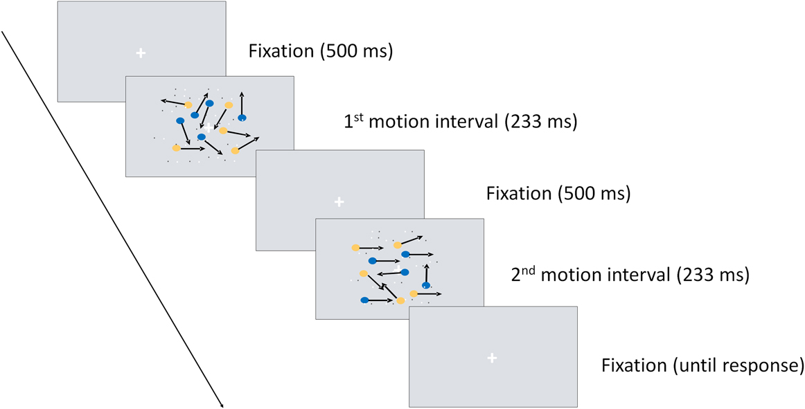
We used a two-interval forced-choice design in which participants had to decide whether the first or the second interval contained coherent motion irrespective of its direction; the other interval contained random motion (see Fig. 2 for an example). We refer to this task as motion discrimination task since the observer has to discriminate between random and coherent motion. After an initial fixation period for 500 ms, the first motion interval was displayed, followed by another fixation period of 500 ms after which the second motion interval appeared. Participants responded after the second interval, by pressing a button to indicate the interval in which they thought coherent motion had appeared. The next trial started after the participant had responded. Participants were instructed to give a correct answer, not a fast answer, and they were provided with acoustic feedback. The participant’s responses guided an adaptive placement of the chromatic contrast (modulation between the gray background and a particular dot color; see Fig. 1) of the next stimulus (Watson & Pelli, Reference Watson and Pelli1983). To obtain contrast thresholds for each participant, we fitted a cumulative Weibull function to the data. Threshold was defined as the contrast at which observers achieved 81% correct responses.
Trial outlook for the two-alternative forced-choice procedure: two motion intervals (one 50% coherent and one random) are presented, and the participant decides which one of the intervals contained coherent motion.

Each observer was involved in both experiments (experiments 1 and 2), and each experiment extended over several sessions (6- to 7-h sessions, on average). After participants consented to participate in the experiment, the color vision test was conducted, and heterochromatic flicker photometry was performed. Subsequently, in several sessions, contrast thresholds for same-polarity RDKs and different-polarity RDKs were obtained.
Color space
To describe the chromatic properties of our stimuli, we use the Derrington-Krauskopf-Lennie color space (Derrington et al., Reference Derrington, Krauskopf and Lennie1984; Brainard, Reference Brainard, Kaiser and Boynton1996), which is an extension of the MacLeod–Boynton chromaticity diagram (MacLeod & Boynton, Reference MacLeod and Boynton1979). In this space, any color is defined by modulations along three different “cardinal” axes: along the achromatic axis, all three cone classes (L, M, and S) are modulated such that the contrast is identical, that is ΔL/L BG = ΔM/M BG = ΔS/S BG, where ΔL, ΔM, and ΔS denote the incremental cone excitations in three cone classes, respectively. L BG, M BG, and S BG indicate the L-, M-, and S-cone excitations of the background. The second direction refers to a modulation along a red–green axis; modulations in this direction leave the excitation of the S cones constant (i.e., ΔS = 0), and the excitation of the L and M cones covaries as to keep their sum constant. Therefore, this axis if referred to as a “constant S-cone axis” (Kaiser & Boyton, Reference Kaiser and Boyton1996) or a “red–green isoluminant” axis (Brainard, Reference Brainard, Kaiser and Boynton1996). Along the third axis, only the S cones are modulated and ΔL = ΔM = 0. Therefore, this axis is often referred to as a “constant L & M cone” axis, or as an “S-cone isoluminant” axis, or as a “tritanopic confusion line.”
Instead of defining the chromatic properties of a stimulus by their respective L-, M-, and S-cone modulations, the stimuli can be defined in terms of the responses of a set of hypothesized mechanisms that are isolated by these stimuli (Brainard, Reference Brainard, Kaiser and Boynton1996; Wuerger et al., Reference Wuerger, Watson, Ahumada, Rogowitz and Pappas2002). The three corresponding mechanisms are two cone-opponent color mechanisms and a luminance mechanism (Fig. 1). One of the two cone-opponent mechanisms is a red–green mechanism that takes the weighted difference between the differential L- and the M-cone excitations. The second cone-opponent mechanism is a yellowish-violet mechanism that takes the weighted difference between the differential S-cone excitations and the summed differential L- and M-cone excitations. The luminance mechanism sums the weighted differential L- and M-cone signals. These orthogonal mechanisms are often referred to as “L + M,” “L − M,” “S−(L + M)” (Derrington et al., Reference Derrington, Krauskopf and Lennie1984). In this paper, we will define the chromatic properties of the stimuli in terms of their modulations in the L, M, and S cones (i.e., as “S,” “L − M,” and “L + M + S”), as described in the first paragraph.
We selected the nominal isoluminant plane at 50 cd/m2, and all colors in this plane have the same luminance. In the DKL color space on the selected isoluminant plane, 0 and 180 deg refer to the end points of the “L−M” direction. The absolute cone coordinates for green (180 deg and radius r = 1) were L = 30.39, M = 19.61, and S = 1.05. The coordinates for red (0 deg and r = 1) were L = 34.45, M = 15.55, and S = 1.05. For modulations symmetric around the white point, the maximum contrast achievable in the L and M cones along the “L−M” direction were 0.06 and 0.11, respectively, and correspond to 1 in all figures. Degrees 90 and 270 refer to the end points along the “S−(M + L)” direction: 90 deg and r = 1 represent violet (L = 32.42, M = 17.58, and S = 1.8), and 270 deg and r = 1 indicate the lime-colored end point (L = 32.42, M = 17.58, and S = 0.31). The maximum available S-cone contrast for our monitor is 0.84, and a radius of 1 in the “S−(M + L)” direction corresponds to an S-cone contrast of 0.706. The Commission International de l'Eclairage chromaticity and luminance values of the gray background were: x = 0.292, y = 0.306, Y = 50 cd/m2. The corresponding cone coordinates were: L = 32.42, M = 17.58, and S = 1.055. Thus, all colors within a circle of radius 1 around the white point were within the gamut of the monitor; this does not mean that colors with a radius >1 were automatically outside the gamut.
To adjust for observers’ individual point of isoluminance, we determined their point of isoluminance by heterochromatic flicker photometry. Since temporal and spatial factors may affect the individual point of isoluminance, we used stimuli as similar as possible to the temporal and spatial layout of our global motion task, that is, we used a random dot pattern stimulus of the same spatial layout as in the main experiments. The dots were modulated between red and green or between yellow and violet (cf. Fig. 1); the modulations were symmetric around the gray background. All observers reported that they could find a setting where the flicker disappeared or almost disappeared. Each observer repeated this selection 10 times reliably; the lowest and highest values were discarded, and the average of the remaining eight measurements was taken (for details see Ruppertsberg et al., Reference Ruppertsberg, Wuerger and Bertamini2003). In the main experiment, the luminance levels of the colored blobs were set to these individually determined luminance levels instead of using the nominal luminance of the gray background.
In order to eliminate a possible effect of luminance artifacts, dynamic two-dimensional luminance noise was added to the motion interval. The Root-mean-square contrast of the luminance noise was 24% (for more details on effective masking parameters see Ruppertsberg et al., Reference Ruppertsberg, Wuerger and Bertamini2003).
Experimental hypotheses
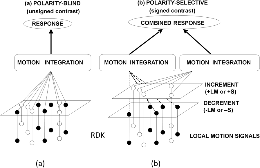
The purpose of our experiments was to test whether the motion integration performed by the visual system is sensitive to the polarity of the local motion signals. In other words, does integration of local chromatic motion signals occur across different polarities, that is, whether it is polarity blind with only the unsigned contrast feeding into the global motion mechanism (Fig. 3a). Alternatively, the integration mechanism may be sensitive to the polarity of the local motion signals, that is, a dynamic motion stimulus may be first segmented based on the polarity cue, and the integration of local motion signals is thus restricted to signals of the same polarity (Fig. 3b). To that end, we measured contrast thresholds for motion discrimination for same-polarity RDKs (experiment 1) and different-polarity RDKs (experiment 2). For same-polarity RDKs, we measured contrast thresholds for three different dot densities (50, 100, and 200 dots) to derive an estimate of the effect of dot density on contrast thresholds. The thresholds for the same-polarity RDKs were then used to predict the thresholds for different-polarity RDKs, assuming that integration is polarity blind. These model predictions were then compared with the observed thresholds for different-polarity RDKs.
Two models of motion integration are depicted. (a) The polarity-blind model is shown, assuming that the motion integration mechanism is not sensitive to the contrast polarity of the local motion signals. (b) The alternative model is shown, assuming that the stochastic random motion stimulus (RDK) is first segregated based on the contrast polarity (i.e., increments vs. decrements) and motion integration mechanisms then act upon the segregated local motion signals.

Experiment 1: same-polarity RDKs
Contrast thresholds for discriminating 50% coherent motion from random motion were measured for same-polarity RDKs. Moving dots were presented on a gray background (midpoint in Fig. 1), and four same-polarity RDKs were used: dots were defined either as LM increments (“red” = +LM), LM decrements (“greenish” = −LM), S increments (“violet” = +S), or S decrements (“lime” = −S). The chromatic contrast (modulation between the gray background and the particular dot color) was varied according to a QUEST procedure, and a cumulative Weibull function was fitted to obtain the threshold contrast, which was defined as the contrast at which the observer’s performance reached 81% correct. Contrast thresholds were obtained for three different dot densities: 50, 100, and 200 dots, yielding altogether 12 different conditions.
Experiment 2: different-polarity RDKs
Different-polarity RDKs were constructed by physically adding same-polarity RDKs (i.e., +LM and −LM; or +S and −S) at their respective threshold contrasts (obtained in experiment 1). For example, to generate a 100-dot different-polarity red–green RDK, the 50-dot RDKs for +LM and −LM were added, with +LM and −LM at their respective threshold contrasts. Contrast thresholds for discriminating coherent motion in the different-polarity RDK were then obtained by simultaneously modulating the contrast of +LM and −LM dots, with the contrasts being yoked in relation to the threshold contrast. As in experiment 1, the yoked contrast was varied according to a QUEST procedure, and a cumulative Weibull function was fitted to obtain the threshold contrast (81% correct). Similarly, to generate a 200-dot different-polarity red–green RDK, the 100-dot +LM and −LM RDKs were added, and the contrast was yoked in relation to their same-polarity thresholds. RDKs containing S increments and decrements were generated accordingly.
Altogether, contrast thresholds for four different conditions were measured in experiment 2: for the two dot densities (100 and 200 dots) and for both color directions (LM and S).
Results
Experiment 1
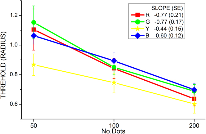
Contrast thresholds for the motion discrimination as a function of dot density are shown in Fig. 4 for all four chromatic conditions (+LM, −LM, +S, and −S). Contrast is expressed as the radius, that is, the distance from the gray background (cf. Fig. 1). To evaluate the effect of dot number on contrast threshold, a straight line was fitted in lin–log coordinates. The dependence on dot density is identical for RDKs defined by LM increments and decrements (slope = −0.77) and very similar for S-cone modulations of negative and positive polarity.
Contrast thresholds for motion discrimination are plotted as a function of dot density for same-polarity RDKs (experiment 1). The dependence on dot density is similar for increments and decrements. Data are averaged over all eight observers. Error bars indicate 2 s.e.m.

Experiment 2
In experiment 2, we measured the contrast thresholds for different-polarity RDKs. The contrasts for the increments and decrements were yoked, according to the threshold ratio obtained with the same-polarity RDKs. That means that the contrast of the different-polarity RDKs, in contrast space normalized to threshold, was modulated along the 45-deg line. For example, we obtained contrast thresholds for the 50-dot +LM and the 50-dot −LM RDK in experiment 1 (cf. Fig. 4); in experiment 2, the ratio between threshold contrasts in the 100-dot different-polarity LM RDKs was fixed to the ratio between these 50-dot LM RDK thresholds. This normalization with threshold was performed in order to ensure that stimuli of different polarities (+LM and −LM; +S and −S) were equally effective in the motion discrimination task in the different-polarity RDKs. Similarly, the 200-dot different-polarity RDKs contained contrasts normalized with the 100-dot same-polarity thresholds. From now on, we will refer to these contrast thresholds as relative contrast thresholds to express the fact that in all mixed-polarity RDKs, the increments and decrements were chosen to be equally effective in the motion discrimination task.
The relative contrast thresholds are shown in Fig. 5. The figures were created by normalizing the same-polarity thresholds to 1 (represented by the dashed horizontal lines) and then plotting the different-polarity thresholds and predictions relative to this normalized value. Error bars indicate 2 s.e.m.
Observed and predicted (assuming the polarity-blind model) relative thresholds are shown for the 100-dot (a, c) and the 200-dot mixed-polarity RDKs (b, d). The upper row shows the data for RDKs defined by LM increments and decrements (a, b); the lower row for S increments and decrements (c, d). Error bars indicate 2 s.e.m.

In Fig. 5a, same-polarity thresholds for the 50-dot RDK are represented by the dashed horizontal line, and the relative thresholds for the 100-dot different-polarity (LM+; LM−) RDKs are shown by the left bar (“OBSERVED”). Thresholds are clearly reduced compared with the 50-dot RDK. This is expected, on account of the increasing number of dots contained in the 100-dot different-polarity RDK; a reduction in contrast threshold per se is not indicative of separate encoding of increments and decrements since a reduction is also observed in the single-color RDKs, when the dot numbers are increased from 50 to 100 dots (cf. Fig. 4; see section “Model predictions”). In Fig. 5b, the left bar shows the observed thresholds for the 200-dot different-polarity (LM+; LM−) RDK, normalized with the threshold for the LM+ and LM− 100 same-polarity RDKs (set to unity; dashed horizontal line). The second row shows the corresponding thresholds for the S-cone stimuli, for the 100-dot different-polarity (Fig. 5c) and 200-dot different-polarity RDKs (Fig. 5d).
In all four mixed-polarity conditions, LM100, LM200, S100, and S200, we observe a reduction in threshold, which may be partly due to the increased number of dots; hence, the threshold reduction itself is not informative about the polarity selectivity (or lack of it) of mechanisms that perform chromatic global motion integration.
Model predictions
To test whether the integrative motion mechanisms are sensitive to the chromatic polarity of local motion signals, we predict the relative contrast thresholds for motion discrimination and compare these with the observed thresholds. If the integration across local motion signals is polarity blind (Fig. 3a), then we expect that the contrast threshold for a 100-dot different-polarity RDK would be the same as the contrast threshold for a 100-dot same-polarity RDK. If polarity does not matter, we should be able to replace—in the different-polarity RDK—the +LM dots with the −LM dots (and vice versa) without changing the performance in the motion discrimination task. This means that the predicted relative threshold for the different-polarity 100-dot RDK would simply be equal to the average of the relative thresholds for the same-polarity 100-dot RDK (+LM and −LM). This is possible, since the dependence on dot density is similar for +LM and −LM (cf. Fig. 4). In the Appendix, we describe in detail how the polarity-blind predictions are derived.
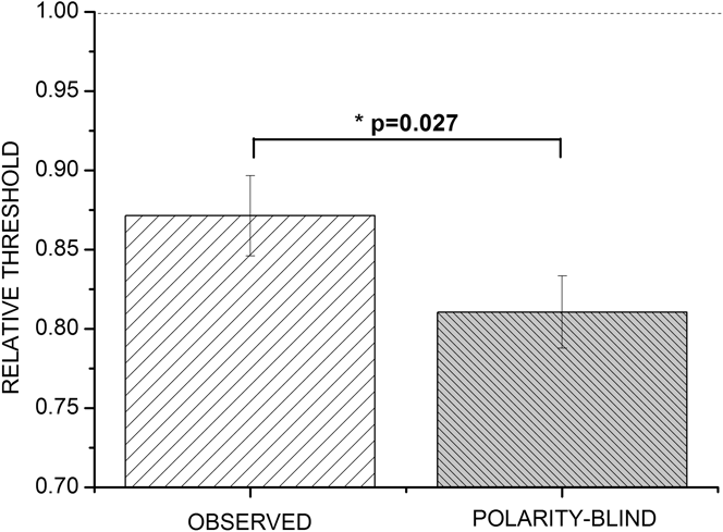
Polarity-blind predictions are shown by the dark bars in Fig. 5a–5d. Fig. 5a shows the predictions for a 100-dot mixed-polarity (LM) RDK. For each observer, the same-polarity relative thresholds for the 100-dot RDK were used (+LM and −LM) to predict the relative threshold for the 100-dot RDK. Fig. 4b shows the corresponding predictions for 200-dot LM RDK; in the second row, predictions are shown for the 100-dot S RDK (Fig. 5c) and the 200-dot S RDK (Fig. 5d), respectively. In all cases, the predicted thresholds (dark bars) are lower than the observed thresholds (light bars).
A within-subject three-way analysis of variance (Matlab statistics toolbox; factor 1: observed thresholds, model predictions; factor 2: chromatic mechanism—LM or S; factor 3: dot density—100 or 200) revealed no significant effects of dot density [F(1,7) = 0.63; not significant (n.s.)] or of chromatic content [F(1,7) = 0.81; n.s.]. Model predictions differed from the observed thresholds significantly [F(1,7) = 7.68; P = 0.0276]. Since none of the interactions were significant, we collapsed the data across chromatic mechanisms and dot densities and replotted them in Fig. 6. Fig. 6 shows that the polarity-blind model can be rejected: the predicted thresholds are systematically smaller than the observed thresholds, for all four experimental conditions (Fig. 5a–5d).
Observed and predicted relative thresholds are collapsed across color and dot density. Error bars indicate 2 s.e.m.

The rejection of the polarity-blind model (Fig. 3a) lends support to the hypothesis that motion integration mechanisms are sensitive to the contrast polarity of the local motion signals and that the output of these polarity-selective mechanisms is combined at a later stage (Fig. 3b). A simple method to determine the amount of summation between two channels is the Quick response-pooling model (Quick, Reference Quick1974), which has been successfully applied to gauge the amount of summation within one sensory modality (e.g., To et al., Reference To, Lovell, Troscianko and Tolhurst2010) as well as between different modalities (e.g., Meyer et al., Reference Meyer, Wuerger, Roehrbein and Zetzsche2005). According to the Quick pooling model (chapter 4.8 in Graham, Reference Graham1989), the responses of the N analyzers to a particular stimulus are pooled according to a Minkowski metric:

In our case, we assumed two analyzers, one for increments and one for decrements, and for each observer and each condition, we determined the pooling factor k; the average pooling factors are quite high, ranging from 2.8 to 6.5 (Fig. 5a–5d), which is indicative of little summation. Pooling factors close to 1 reflect linear summation of the individual responses; in the limiting case, when k approaches infinity, the threshold for the combined stimulus is determined by the most sensitive channel (Graham, Reference Graham1989).
Discussion and conclusion
We utilized RDKs to gauge the effect of chromatic contrast polarity on the integration of local motion signals, by measuring contrast thresholds for single-polarity and mixed-polarity RDKs. Our main finding is that the observed mixed-polarity thresholds were systematically larger (Fig. 5a–5d) than the thresholds for the single-polarity RDKs. This is consistent with our hypothesis that motion integration is sensitive to the polarity of the local motion signals (Fig. 3a). Numerous studies using simple detection tasks have demonstrated that increments and decrements along the two isoluminant chromatic directions (L–M; S) are processed separately in ON and OFF channels and not via linear cone-opponent mechanisms (McLellan & Eskew, Reference McLellan and Eskew2000; Sankeralli & Mullen, Reference Sankeralli and Mullen2001). Our current study extends these findings and suggests that separate ON and OFF mechanisms not only mediate simple detection tasks but that at an early level of motion analysis, increments and decrements are processed separately and that the integration mechanisms are also selective to the chromatic polarity of the local motion signals. For form perception, the evidence on the polarity selectivity of global integration mechanisms is controversial (Rentzeperis & Kiper, Reference Rentzeperis and Kiper2010; but see also Wilson et al., Reference Wilson, Switkes and De Valois2004); a direct comparison with the current results is difficult since we used a stochastic motion stimulus, whereas the above studies used static glass patterns, and it is likely that different mechanisms are involved in the analysis and the integration of static and moving local elements.
To assess the amount of summation between the ON and OFF channels (+LM and −LM; +S and −S), we determined the summation constants assuming a Quick pooling model; we obtained summation factors larger than previously reported, which suggests that little summation occurs across the ON and OFF channels in the motion discrimination task employed in our experiments.
Appendix A
Quantitative “polarity-blind” predictions
Here, we assume that local motion signals defined by increments or decrements are not processed by separate motion mechanisms. The following example shows how the relative contrast threshold for the 100-dot LM different-polarity RDK is predicted based on the thresholds for same-polarity RDKs.
We first define the thresholds for the different conditions (also plotted in Fig. 4). C +LM50 and C −LM50 denote the threshold contrast for the same-polarity 50-dot RDK for the +LM and −LM conditions, respectively; C +LM100 and C −LM100 denote the corresponding thresholds contrast for the same-polarity 100-dot RDKs. Since we are only interested in the threshold reduction with an increase in dot density (increasing from 50 to 100 dots), we calculate relative thresholds; rC +LM100 denotes the relative threshold contrast for the same-polarity 100-dot +LM RDK:

These relative thresholds indicate how much thresholds are reduced by doubling the number of dots in the RDK. Since the dependence on number of dots is the same for +LM and −LM (cf. Fig. 4), the predicted relative threshold for the 100-dot different-polarity RDK is simply obtained by taking the average:

The predictions for the 200-dot different-polarity RDKs are derived accordingly, scaled in threshold units for the 100-dot same-polarity RDKs.
Acknowledgments
This project was funded by the Wellcome Trust No. GR/058513 (to S.M.W. and M.B.). A.R. and J.M. were employed as research assistants on the WT grant. S.M. assisted with the data collection during her internship at the University of Liverpool.