3.1 Transition from a steady vertical trajectory to a steady oblique one

When the Galileo number is below the first bifurcation and no magnetic field exists, a free sphere will travel with vertical trajectory regardless of the density ratio. No wake instability will occur and only the solid model exists in the fluid–solid system. A series of cases at $m=0.5$ with different Galileo numbers are first simulated to get their final stable states. Then an external vertical magnetic field is imposed. Figure 2 shows that the sphere with a steady vertical trajectory becomes steady oblique. Obviously, the instability occurs with an external vertical magnetic field. Generally, the magnetic field will play a damping role in a free rising bubble with an oscillatory path, as reported in experiment (Zhang, Eckert & Gerbeth Reference Zhang, Eckert and Gerbeth2005) and simulation (Zhang & Ni Reference Zhang and Ni2017). They reported that an external vertical magnetic field was used to diminish the asymmetry of the vertical vortex pairs. It is noted that the wake structure behind the bubble determines its trajectory (Ern et al. Reference Ern, Risso, Fabre and Magnaudet2012) and more symmetric vertical vortex pairs will lead to a more stable trajectory. Hence, their results showed that the oscillatory path of a bubble was transitioned to a more rectilinear trajectory. The oscillatory bubble mainly relates to the fluid model, which involves the wake instability. However, the present fluid–solid system only has the solid model and figure 2 shows that the interaction between the magnetic field and the solid model facilitates the transition onset here.

Figure 2.

Horizontal velocity $V_{h}$ and rotation velocity $W_{h}$ of the sphere at $m=0.5$ with different Galileo numbers versus the interaction parameter. The $V_{h},W_{h}$ are scaled with $U_{0}$ and $U_{0}/d$ , respectively. (a) Horizontal velocity. (b) Horizontal rotation velocity.

A weakly nonlinear expansion method in Fabre et al. (Reference Fabre, Tchoufag and Magnaudet2012) reported that the horizontal rotation played a key role in the transition onset from a steady vertical trajectory to a steady oblique one without a magnetic field. Hence, some numerical experiments are designed about rotation degrees of freedom at $G=150,m=0.5$ with different interaction parameters. As shown in figure 2, when $N>N_{c}\approx 0.4$ , the transition occurs and a horizontal velocity exists. Figure 3(a,b) shows comparison results by freezing all rotation degrees of freedom of the sphere. No horizontal velocity occurs at a small magnetic field $N=0.5$ , while there is a transition onset at a large magnetic field $N=2$ . These results indicate that both the rotation and the translation degrees of freedom can facilitate the transition onset and the rotation one plays a key role, which agrees with the conclusions found without a magnetic field in Jenny, Bouchet & Dušek (Reference Jenny, Bouchet and Dušek2003) and Fabre et al. (Reference Fabre, Tchoufag and Magnaudet2012). Furthermore, a 1 % perturbation of horizonal rotation velocity at $N=0.5$ is added on the sphere with different interaction parameters. Figure 3(c) shows that the perturbation is suppressed when $N<N_{c}$ or it is quickly enlarged when $N>N_{c}$ . These results imply that the perturbation can only grow when the magnetic field is beyond a critical value $N_{c}$ .

Relative to the reference frame which is fixed in the centre of the sphere and has the same translation velocity $\boldsymbol{v}_{s}$ , the original free motion with $G<156$ in the absence of a magnetic field is equivalent to a flow past a fixed sphere, for which the flow is steady and axisymmetric and a separated bubble is attached at the rear of the sphere. After the fluid–solid system reaches its stable state, an external vertical magnetic field is imposed. A diagram in figure 4(a) shows that the flow field is affected by the magnetic field. With some vector operations, equation (2.5) can be reformed as $\unicode[STIX]{x1D735}\boldsymbol{\cdot }\unicode[STIX]{x1D735}\unicode[STIX]{x1D719}=\unicode[STIX]{x1D735}\boldsymbol{\cdot }(\boldsymbol{u}\times \boldsymbol{B})=\boldsymbol{B}\boldsymbol{\cdot }\boldsymbol{\unicode[STIX]{x1D714}}=0$ , since the flow is axisymmetric and no vertical vorticity exists. So $\unicode[STIX]{x1D719}$ is zero (or a constant) and no current is induced from the electric potential in Ohm’s law (2.3). The Lorentz force can be rewritten as $\boldsymbol{F}_{L}=-N\boldsymbol{u}_{\bot }B^{2}$ , which always prevents the flow that is not parallel to the magnetic field. Here, $\boldsymbol{u}_{\bot }$ represents the velocity components normal to $\boldsymbol{B}$ . Due to the Lorentz force, two relatively stagnant regions ahead of and behind the sphere occur, as shown in figure 4(a). The streamlines compactly wrap the sphere without a magnetic field and now they are loosened by the Lorentz force. Consequently, the stability of the fluid–solid system is decreased. As implied in figure 3(c), increasing the magnetic field destabilizes the fluid–solid system and the transition occurs when the magnetic field exceeds a critical value $N_{c}$ . Figure 2 indicates that the smaller the Galileo number of a case is, the larger the critical value it has. This is because a small Galileo number case has a smaller separated bubble (Johnson & Patel Reference Johnson and Patel1999). That is to say, the sphere is more compactly wrapped by the streamlines and it needs a larger magnetic field to decrease the stability of the fluid–solid system.

Figure 3.

Numerical experiments at $G=150,m=0.5$ affected by a magnetic field. ‘FR’ and ‘P’ stand for ‘freeze rotation’ and ‘perturbation’, respectively. The $V_{h}$ and time are scaled with $U_{0}$ and $d/U_{0}$ , respectively. (a) Freeze all rotation degrees of freedom at $N=0.5$ . (b) Freeze all rotation degrees of freedom at $N=2$ . (c) A 1 % perturbation of horizonal rotation velocity at $N=0.5$ is added on the sphere with different interaction parameters.

Figure 4.

Understanding the transition onset of a horizonal velocity. (a) A compact model for the influence of the magnetic field. ‘HP’ and ‘LP’ stand for ‘high pressure’ and ‘low pressure’, respectively, due to the Lorentz force. The high pressure in the HP region pushes away the streamlines and the Lorentz force in the LP region directly pulls away the streamlines. (b) A positive feedback effect for the fluid–solid system. (c) Three-dimensional streamlines projected onto the symmetric plane at $Re=250$ with $N=0$ in a fixed sphere case.

Assuming that one is at the centre of the sphere to observe the flow field, an axisymmetric recirculation exists behind the sphere. Jenny et al. (Reference Jenny, Bouchet and Dušek2003) reported that the instability of a free sphere degrees of freedom was associated with the azimuthal wave perturbations of the flow. When the stability of the fluid–solid system is decreased by the magnetic field ( $N>N_{c}$ ), these perturbations will evolve and the axisymmetric recirculation is broken, which results in a small tilt shift of the recirculation. Actually, such a tilt corresponds to a torque on the original non-rotating sphere, as shown in figure 4(c). Such a torque can be fully compensated by the sphere rotation. Furthermore, the rotation of the sphere will enlarge the tilt of the recirculation, which will exert a net torque on the sphere. This net torque needs a larger rotating velocity of the sphere to compensate its effect. Finally, the sphere will stay in a new steady state, for which the hydrodynamic torque and lift remain zero. Hence, the positive feedback effect shown in figure 4(b) exists, which transitions the fluid–solid system into a new equilibrium state.

3.2 The wake structures at the rear of the sphere

The wake structures behind the sphere of figure 2 are analysed in detail in this section. Lighthill (Reference Lighthill and Rosenhead1963) proposed that convergence of skin friction lines was a criterion of a three-dimensional flow separation. Skin friction lines can clearly show flow traces at the rear of the sphere, which help to visualize the wake structures. Figure 5 shows various wake structures affected by different interaction parameters.

Figure 5.

Four types of skin friction lines at $G=150,m=0.5$ affected by different interaction parameters. ‘O’ and ‘S’ indicate the centre of the sphere and the stagnation point, respectively. (a)  $N=0$ . (b)  $N=0.25$ , type I. (c)  $N=0.5$ , type II. (d) Case comparison with $G=165,m=0.5,N=0$ . (e)  $N=1.2$ , type III. (f)  $N=2$ , type IV.

When $N<N_{c}$ , the transition onset does not occur. The wake structures behind the sphere are still axisymmetric, as shown in figure 5(a,b). Such an axisymmetric wake is unable to generate any side force on the sphere and the sphere rises vertically. Increasing the magnetic field, the compact model in figure 4(a) indicates that the stability of the fluid–solid system is decreased. Then a transition occurs when the magnetic field exceeds a critical value $N_{c}$ and the fluid–solid system goes into a new equilibrium state with a positive feedback effect in figure 4(b). If we stand on the centre of the sphere to observe the flow field (non-inertial frame), it has a similar wake structure with a flow past a fixed sphere at $210<Re<270$ , as shown in figure 4(c). The topological structure of the streamlines has a small left spiral and large right spiral and they are tilted behind the sphere. The corresponding skin friction lines are shown in figure 5(c), which shows that the stagnation point shifts from the centre because of the tilt of the recirculation. Furthermore, figure 5(d) shows the same wake structure as figure 5(c), but without a magnetic field. Note that the first bifurcation is about $G=156$ and the magnetic field shifts the transition onset into a lower critical threshold of the Galileo number. Ern et al. (Reference Ern, Risso, Fabre and Magnaudet2012) claimed the wake of the fixed sphere would provide useful insight into the vortex dynamics of the freely moving body. The wake structures of a flow past a fixed sphere affected by a streamwise magnetic field in Pan et al. (Reference Pan, Zhang and Ni2018) or a transverse rotation of the sphere in Giacobello, Ooi & Balachandar (Reference Giacobello, Ooi and Balachandar2009) indicated that both the left and right spirals in figure 4(c) can be dismissed by these two effects. So further increasing the magnetic field, figure 5(e) indicates that only the small left spiral disappears while both these two spirals disappear in figure 5(f). The detailed Lorentz force action on the two spirals can be found in Pan et al. (Reference Pan, Zhang and Ni2018). As shown in figure 4, a positive feedback effect includes a transverse rotation of the sphere. The existence of the transverse rotation will facilitate the fluid–solid system to quickly change to a new equilibrium state, which can be seen in figure 3(b) compared with the case of no rotation.

As shown above, the rising sphere at $G=150$ and $m=0.5$ has four kinds of wake structures under the influence of a vertical magnetic field. Assume that one is at the centre of the sphere to observe the flow field. Since types I, II and III still have recirculation, the tilt of the recirculation will convert the azimuthal vorticity into a streamwise vorticity. With the existence of a positive feedback effect, by increasing the magnetic field, the tilt will increase quickly, which means that more streamwise vorticity is converted behind the sphere. When the flow pattern is in type IV, no recirculation exists, so the positive feedback effect is excluded. Now the Lorentz force always suppresses the streamwise vorticity and the intensity of the streamwise vorticity will decrease. Such a variation of the streamwise vorticity is shown in figure 6(b). Actually, the flow in type I is axisymmetric and no streamwise vorticity exists. The topological structures of the streamwise vorticity in types II, III and IV are the same. They are plane symmetric with a counter-rotating vortex pair, as shown in figure 6(a), which are only different in the intensity affected by the magnetic field. But the skin friction lines show four different topological structures, which implies more flow field information to analyse the fluid dynamics. Furthermore, figure 7 shows that the streamwise vorticity can induce an induced flow. With the law of interaction, a lift force corresponding to this induced flow will be produced in the symmetric plane, which will drive the sphere. Thus a horizontal velocity occurs to compensate the lift force. Since the magnitude of the force determines the horizontal velocity, the horizontal velocity has an identical variation trend to the streamwise vorticity, as shown in figures 6(b) and 8.

Figure 6.

Streamwise vorticity behind the sphere at $G=150,m=0.5$ affected by a magnetic field. (a) The isosurfaces of streamwise vorticity with $\unicode[STIX]{x1D714}_{z}=\pm 0.4$ at $N=2$ in a front view. (b) The maximal magnitude of streamwise vorticity affected by different interaction parameters.

Figure 7.

Cross-section plot of vertical vortical structures at $z=1d$ behind the sphere with $G=150$ , $m=0.5$ , $N=1.2$ . The dashed line represents the sphere.

An interesting phenomenon in figure 8 is that the inflection point of the horizontal rotation velocity is $N=2$ , which is different from that of the horizontal velocity $N=1.2$ . The torque exerting on the non-rotating sphere is determined from the viscous stress force on the sphere surface, since the pressure force has no contribution. This torque is fully compensated by the sphere rotation. The tilt of skin friction lines at the rear of the sphere reflects the magnitude of viscous stress force and is closely related to the tilt of recirculation behind the sphere. As can be seen in figure 5, the tilt of skin friction lines is increasing from type I to III, so the horizontal rotation velocity becomes large. However, it is not clear for type IV, since there is no recirculation behind the sphere. It is noted that the skin friction lines are in connection with the flow pattern behind the sphere. Hence, the tilt of the skin friction lines can be quantitatively measured by the angle $\unicode[STIX]{x1D703}$ between the vertical direction and the direction along the thread of streamwise vorticity, as shown in figure 9(a). Figure 9(b) plots the variation of angle $\unicode[STIX]{x1D703}$ affected by different magnetic fields, which determines the variation trend of the horizontal rotation velocity, as shown in figure 8.

Figure 8.

Horizontal velocity $V_{h}$ and rotation velocity $W_{h}$ of the sphere at $G=150$ , $m=0.5$ affected by different interaction parameters. The $V_{h},W_{h}$ are scaled with $U_{0}$ and $U_{0}/d$ , respectively.

Figure 9.

The angle $\unicode[STIX]{x1D703}$ between the vertical direction and the direction along the thread of streamwise vorticity at $G=150,m=0.5$ affected by a magnetic field. ‘O’ indicates the centre of the sphere. (a) The isosurfaces of streamwise vorticity with $\unicode[STIX]{x1D714}_{z}=\pm 0.4$ at $N=2$ in a side view. (b) The angle $\unicode[STIX]{x1D703}$ affected by different interaction parameters.

In figure 6(b), when $N<1.2$ , the flow patterns are in regimes I, II and III. For such regimes, the magnetic field facilitates the transition onset and the positive feedback effect exists, which will make the streamwise vorticity change quickly. When $N>1.2$ , the flow pattern now is in regime IV, where no positive feedback effect exists and the Lorentz force always suppresses the streamwise vorticity and slowly decreases it. It is noted that the Lorentz force will damp a flow that is non-parallel to the magnetic field, which actually prevents the tilt of the recirculation. So there is competition between the suppression of the Lorentz force and the positive feedback effect on the tilt of recirculation behind the sphere. When the positive feedback effect is dominant, the tilt is enlarged. With an increasing magnetic field, the suppression of the Lorentz force becomes strong enough to prevent the development of the tilt caused by the positive feedback effect. For the case $G=110$ , the fluid–solid system is more stable than the case of $G=150$ . With the competition between the suppression of the Lorentz force and the positive feedback effect, no wake in types III and IV occurs. In the present investigations, the free sphere first attains its stable state without a magnetic field, then an external vertical magnetic field is imposed. Furthermore, for a sufficiently large magnetic field, a perturbation creates a small tilt of the recirculation behind the sphere. Since the Lorentz force is large enough, it prevents the tilt of the recirculation and the positive feedback effect can not be evolved any longer. Now the wake will remain axisymmetric and no horizontal velocity exists. Such cases correspond to a sufficiently large magnetic field situation as in figure 2. It is interesting that the magnetic field has a double effect on the fluid–solid system, which will facilitate or prevent the tilt of the recirculation in term of different magnetic field intensities. For the case $G=100$ in figure 2, considering the double effect of the magnetic field, on the one hand, it needs a larger magnetic field to facilitate transition onset because the sphere is more compactly wrapped by streamlines. On the other hand, this large magnetic field also plays a suppressing role and now the suppression of the large Lorentz force is more dominant than that of the positive feedback effect, which will prevent the tilt of the recirculation. Hence, no transition onset will occur and the horizontal velocity remains zero.

Figure 10 shows three kinds of typical axisymmetric flows at $G=150,m=0.5$ , when the magnetic field is absent, close to a critical value, or sufficiently large. Here, the streamlines are plotted with the relative fluid velocity. It is assumed that one is at the centre of the sphere and observing the recirculation flow at the rear of the sphere. In figure 10(a,b), the streamlines at the position indicated by a red arrow are pulled away from the recirculation by the Lorentz force $\boldsymbol{F}_{L}=-N\boldsymbol{u}_{\bot }B^{2}$ and flow downstream. The sphere is compactly wrapped by streamlines at $N=0$ and these streamlines are loosened by the Lorentz force, which will destabilize the fluid–solid system. A compact model is given to explain the transition onset in § 3.1. The pressure contour and streamlines in figure 10(c) are not perfectly symmetric. This is because the suppression of the large Lorentz force is more dominant than the positive feedback effect and a small tilt of the recirculation caused by a perturbation can not be evolved. Furthermore, the change of the recirculation bubble, such as recirculation length and separation angle affected by a magnetic field in a axisymmetric flow zone is similar to a flow past a fixed sphere case at $Re=150$ in Pan et al. (Reference Pan, Zhang and Ni2018).

Figure 10.

Pressure contours and streamlines in the symmetric plane at $G=150,m=0.5$ with different interaction parameters. The streamlines are plotted with the relative fluid velocity $\boldsymbol{u}_{r}=\boldsymbol{u}-\boldsymbol{v}_{s}$ . The red arrow indicates the same position. (a) Without a magnetic field at $N=0$ . (b) Close to a critical magnetic field at $N=0.35$ . (c) With a sufficiently large magnetic field at $N=30$ .

3.3 Independence of the density ratio

The above results are relative to the density ratio $m=0.5$ . Fabre et al. (Reference Fabre, Tchoufag and Magnaudet2012) reported the primary bifurcation was independent of the density ratio without a magnetic field. So now we check the role of the density ratio in the three-dimensional parameter space $\{m,G,N\}$ . A wide density ratio $m$ parameter space [0.01,10] with different Galileo numbers versus the interaction parameter are simulated. A total of 159 cases are simulated and the results show that the physical behaviour of the free sphere is also independent of the density ratio when affected by the magnetic field, regardless of whether there is a transition onset or not. The wake or trajectory of the freely moving sphere is only determined by the Galileo number and the interaction parameter. Hence, the parameter space $\{m,G,N\}$ can reduce to $\{G,N\}$ , when $G<156$ . The results of $m=0.5$ in the above sections can be extended to any density ratio, so the results of other density ratios are not repetitively plotted. The independence of the density ratio can be easily understood in Newton motion equations (2.7) and (2.8). The sphere has a steady state in the final state. Thus the time derivative term disappears at last and the remaining equations are free of the density ratio.

Figure 11.

The vertical velocities of different Galileo numbers $G$ and density ratios $m$ . The $V_{z}$ is scaled with $U_{0}$ . (a) The vertical velocities are agglomerated into a point for a certain magnetic field, when $N>1$ . An agglomerated curve line consists of these points. (b) Linear dependence of the vertical velocity versus $N^{-1/4}$ , when $N>1$ .

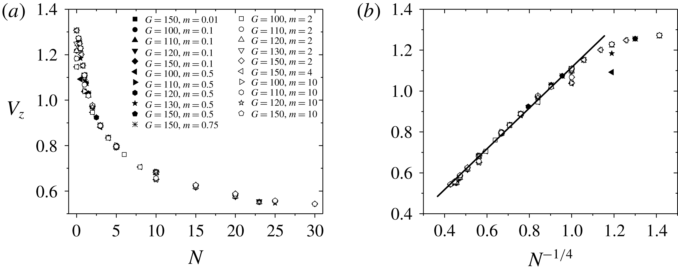
The vertical velocity is also plotted in figure 11(a). It is clearly seen that when $N>1$ , the vertical velocities of different Galileo numbers are agglomerated into a point for a certain magnetic field, which means that it is not only independent of the density ratio, but also the Galileo number. We call this the ‘agglomeration phenomenon’. The vertical velocity in the final state is controlled by (2.7). It is simplified as

(3.1) $$\begin{eqnarray}0=\frac{6}{\unicode[STIX]{x03C0}}\int _{\unicode[STIX]{x1D6E4}}\unicode[STIX]{x1D749}\boldsymbol{\cdot }\boldsymbol{n}\,\text{d}S\boldsymbol{\cdot }\boldsymbol{e}_{\Vert }+\text{sgn}(m-1).\end{eqnarray}$$

Here, $\boldsymbol{e}_{\Vert }$ denotes the vertical direction. As in the analysis in figure 4(a), with the suppression of the Lorentz force, a high pressure zone and a low pressure zone will occur. Therefore, when affected by a strong magnetic field, the pressure drop contribution of the stress force $\unicode[STIX]{x1D70F}_{i,j}=-p\unicode[STIX]{x1D6FF}_{i,j}+(2/G)(\unicode[STIX]{x2202}_{i}u_{j}+\unicode[STIX]{x2202}_{j}u_{i})$ is dominant. The second term related to the Galileo number can be ignored. It is noted that for a small Galileo number, the contribution of the second term in stress force increases and the data point will have little deviation from the agglomerated curve line.

A simple drag law $C_{d}\propto N^{1/2}$ is found for the flow past a sphere affected by a strong streamwise magnetic field (Pan et al. Reference Pan, Zhang and Ni2018). The law is also suitable for the present research if we stand on the sphere centre to observe the flow field. In the vertical direction, the balanced relation among the drag force, gravity and buoyancy gives the formula

(3.2) $$\begin{eqnarray}\sqrt{N}\boldsymbol{\cdot }{\textstyle \frac{1}{2}}\unicode[STIX]{x1D70C}u_{z}^{2}\boldsymbol{\cdot }\unicode[STIX]{x03C0}R^{2}\sim |\unicode[STIX]{x1D70C}_{s}-\unicode[STIX]{x1D70C}|\boldsymbol{\cdot }{\textstyle \frac{4}{3}}\unicode[STIX]{x03C0}R^{3}\boldsymbol{\cdot }g,\end{eqnarray}$$

where $R$ is the sphere radius. Substitute the dimensionless vertical velocity $V_{z}=u_{z}/U_{0}$ into the equation and simplify it to get a scaling law:

(3.3) $$\begin{eqnarray}V_{z}\sim N^{-1/4}.\end{eqnarray}$$

The data points in figure 11(a) are replotted in figure 11(b). It is clearly seen that the vertical velocity is linear dependent on $N^{-1/4}$ , when $N>1$ .

Figure 12.

Map of regimes for wake patterns at the rear of the sphere in the $\{G,N\}$ plane. Assume that one is at the centre of the sphere to observe the flow field in the rear of the sphere. Regime I is the steady axisymmetric state with an attached separation bubble. The pattern in regime II is the steady plane symmetric with small and large spirals in the recirculation region. Regimes III and IV are also steady plane symmetric, for which the small spiral in regime III disappears and both small and large spirals disappear in regime IV. ▫, ♢, ▵ and $\star$ represent calculated data points.