

1 Introduction
As the baby boom starts to retire, the question of the adequacy of retirement income is growing more important. In addition to demographic trends, concerns over the future of Social Security and the downward trend in traditional defined benefit pension provision have brought more attention to the importance of private saving for funding retirement income. The adequacy of retirement resources depends not only on how much wealth a household accumulates, but also on decisions on how to allocate and spend this wealth after retirement. Uncertainty about the length of life is crucial in decision making about allocating and spending down wealth. Annuities can provide an important form of insurance in dealing with this uncertainty, but, unfortunately, economic research has indicated that individuals appear to underutilize private annuities.
Much of the public policy toward retirement savings has used the tax code to encourage savings without encouraging retirees to use this savings to purchase annuities. New proposals, however, have introduced targeted incentives to increase annuitization (see, for example, the Lifetime Pension Annuity for You Act of 2007). Our goal is to provide a prognosis for success from two types of such initiatives: (1) a partial exemption of annuity income from taxable income; and (2) a refundable tax credit based on the amount of annuity income received.
We evaluate the responsiveness of annuitization decisions to subsidies using dynamic programming techniques, which have been widely employed in studying annuity markets. We find that targeted incentives are likely to substantially increase private annuitization with a baseline estimated increase in annuitization on the order of $50,000 on average for retired couples, though subject to considerable uncertainty. Our results also indicate that this increase will occur at relatively modest cost to the government in terms of forgone tax revenues, with estimates of the steady-state revenue costs of less than 10–15 cents per dollar of additional annuitization over the entire life of each retired cohort. One difference in the policies is that the benefits of exempting annuity income from taxation are skewed towards relatively well-to-do retirees whereas the refundable tax credit induces annuitization across a broader cross section of retired households.
We emphasize that our results should be interpreted with some caution since the dynamic programming techniques underlying our estimates are the same techniques that motivate the so-called “annuity puzzle:” the models over-predict how much households annuitize. However, our focus on changes in – rather than levels of – annuitization partially assuages concerns about the techniques, and we explicitly offer some plausible conditions under which this approach is valid.
The paper proceeds as follows. The second section briefly reviews existing research on the annuity puzzle. The third section discusses issues of policy design for increasing annuitizaton. The fourth and fifth sections analyze two particular policy proposals, one based on tax exemptions and modeled on recently proposed legislation, and one based on a refundable tax credit. In the fourth section, we present Money's Worth estimates based on market prices, and we compute the effect of the two policies on these Money's Worths. The fifth section incorporates this pricing information into an “Annuity Equivalent Wealth” dynamic programming model with an extensive annuitization margin to assess the policies' potential efficacy. The final section summarizes the policy implications of our analysis and broadly considers other possible approaches to increasing annuitization.
2 A Brief Review of Research on the Annuity Puzzle
A brief review of previous research on annuity markets and the annuity puzzle provides context for our analysis. The “annuity puzzle” is the observation that households appear to annuitize far less wealth than economic analysis suggests they should. Yaari (Reference Yaari1965) showed that full annuitization is optimal in the absence of loading or bequest motives. His theoretical contributions have been extended by Davidoff et al. (Reference Davidoff, Jeffrey and Peter2005), who show that optimizing individuals should make extensive use of annuity markets under quite general conditions.
In practice, however, private annuity markets are quite thin. Using wealth data from the Health and Retirement Survey (HRS),Footnote 1 as of 2000, Poterba et al. (Reference Poterba, Joshua, Steven and David2003) report extremely low levels of (privately) annuitized wealth. For example, the median male between the ages of 63 and 67 has no privately annuitized wealth. Johnson et al. (Reference Johnson, Leonard and Deborah2004) use panel features of the HRS and find that, among individuals with defined contribution (DC) retirement plans who left their job after age 65, only 10% actually converted their DC accumulations into annuities.
Insurance industry data corroborates the thinness of annuity markets. From American Council of Life Insurance data, Brown (Reference Brown2000) reports that less than 4% of individuals with Social Security income also receive private annuity income. Data on deferred annuity sales are also available (see, e.g., NAVA (2005)), but Reichenstein (Reference Reichenstein2002) reports that 98% of individuals who purchase deferred annuities do not convert them into life annuities. Furthermore, the market for immediate annuities is quite thin, with sales of only $5.9 billion in 2006 (LIMRA, 2007), a figure which includes both life annuities and period certain annuities.
James and Vittas (Reference James and Vittas2004) note that thin private annuity markets are an international phenomenon by examining markets in Canada, Australia, Israel, and Singapore, for example. Interestingly, Chile and the United Kingdom, both of which have pension systems with mandatory annuitization of some forms of savings, have more substantial annuity markets (see Finkelstein and Poterba, 2004, on the thinness of the “voluntary” U.K. market).
Mitchell et al. show that unfavorable pricing alone cannot resolve the annuity puzzle. They calculate “Money's Worths” (MWs) – the ratio of the premium to the expected value based on expected mortality and interest rates – and find loads of about 15–20 cents for the average retiree in U.S. annuity market; they attribute about half of the load to adverse-selection. They then use dynamic programming techniques – akin to the “Annuity Equivalent Wealth” technique we use – to find the utility value of annuitization for retirees. They find annuitization values high enough that individuals should readily purchase annuities, despite this less-than-fair pricing.
Other suggested solutions to the annuity puzzle include the existence of pre-annuitized wealth such as Social Security wealth (Mitchell et al. Reference Mitchell, James, Mark and Jeffrey1999); within-household risk pooling for married couples (Brown and Poterba, Reference Brown and Poterba2000); and bequest motives (Friedman and Warshawsky, Reference Friedman and Mark1990).Footnote 2 Even accounting for within-household risk sharing and observed levels of pre-annuitized wealth, dynamic optimization techniques indicate that substantial annuitization should be optimal. Strong enough bequest motives can certainly resolve the puzzle. However, the empirical evidence is decidedly mixed as to the relationship between bequest motives and annuitization decisions: Brown (Reference Brown2001) does not find a significant relationship between the stated desire to leave bequests and the stated intention to annuitize DC plan assets upon retirement; and Johnson et al. (Reference Johnson, Leonard and Deborah2004) note that childless adults are no more likely to annuitize assets from DC balances.
Dushi and Webb (Reference Dushi and Anthony2004) extend the “Annuity Equivalent Wealth” (AEW) techniques used in the literature so that households choose when, how much, and how many times to annuitize, as opposed to earlier literature which largely focused on a one-time decision about whether to annuitize all wealth. This added flexibility can substantially delay annuitization to ages beyond those in the HRS. But, while delay may explain the paucity of annuitization in the HRS, it cannot explain the broader pattern of underdeveloped annuity markets.
The annuity puzzle recommends caution in employing the AEW framework for policy analysis. The divergence between predicted and actual annuitization patterns suggests that the AEW framework neglects some important aspect of the annuitization decision. Nevertheless, the AEW framework is useful for our purposes for at least two reasons. First, despite the annuity puzzle, Brown (Reference Brown2001) shows that the AEW framework does predict households' intentions to annuitize. Using the HRS data for 1992, he estimates that a 1% increase in AEW leads to nearly a 1% increase in the stated intention to annuitize. Second, while the optimization techniques underlying AEW calculations are likely to mis-represent annuitization levels, they may still be useful as guides for predicting changes in behavior. Appendix B offers some simple conditions under which our technique is valid despite overpredicting annuitization levels.
3 The Analytics of Subsidizing Annuitization
The public policy challenge for ensuring retirement income adequacy needs to address both the level of household saving and how households finance consumption in retirement. Over the past few decades, government policies such as the expansion of 401(k) plans have provided incentives for retirement savings but have not emphasized the importance of using life annuity markets. Indeed, the trend toward defined contribution pension plans away from defined benefit pensions will reduce households' annuitized wealth unless households annuitize their defined contribution assets. Recently, policy-makers have proposed tax incentives to encourage annuitization. In the remainder of this section, we first discuss the current income taxation of annuities and then address general issues in designing public policy to encourage annuitization. We apply our analysis to specific policy proposals in Sections 4 and 5.
3.1 Taxation of Annuities
A major tax distinction for annuity contracts is between “qualified” and “non-qualified” purchases. Qualified refers to an annuity purchased within a tax-advantaged savings vehicle, such as a 401(k) or Individual Retirement Account (IRA). For such annuities, the entire payment from the annuity is taxable since all withdrawals from such accounts are fully taxable. In contrast, for Roth-styled (or after-tax) IRAs, the entire annuity payment is exempt from tax. Non-qualified annuities refer to annuity contracts purchased with after-tax dollars. The amount of money contributed to the annuity establishes the taxpayer's basis (or principal) in the annuity. During the accumulation phase of a non-qualified deferred annuity, the investment returns on the contribution to the annuity are not taxed. Instead, the taxation on the “inside buildup” in the annuity is tax-deferred. For both deferred and immediate annuities, a portion of the payment from the annuity is the return of basis to the taxpayer and is not subject to income taxation.Footnote 3 This portion depends on the annuitant's life expectancy when the assets are annuitized and the type of payments that will be received from the annuity (e.g., fixed versus variable payments). The remainder of the annuity payment faces ordinary income tax rates, even when the underlying assets held by the insurance company yield capital gains or dividends that would have faced lower marginal tax rates had the annuitant invested in these assets directly.
3.2 Rationales for Policy Intervention
One rationale for government intervention in annuity markets is to ameliorate adverse selection loads caused by informational asymmetries. A second rationale is moral hazard: since the government effectively provides some degree of assistance for individuals who outlive their resources, individuals may tend to annuitize too little private wealth, so that the rest of society bears part of the cost of the individual's good fortune to live a long life. By encouraging annuitization, the government may reduce these social costs.
A third rationale is paternalistic: many people may naturally underestimate their need for insurance. Public policy can have two beneficial effects in this regard. First, by lowering the price of annuities, people might become more likely to purchase them. Second, the government policy may play an informational role in signaling to people that private annuities are a useful financial product. While our estimates below focus on the first of these effects, the informational role of public policy is potentially important, though the effects are hard to quantify. For non-qualified annuities, there is a fourth rationale for subsidizing annuity purchases: it can help to offset the disparity between the tax treatment of capital-gains and dividend income and the tax treatment of annuity income generated by the same underlying assets.
We focus solely on interventions which encourage people to annuitize wealth, so these policy rationales are best thought of as applying to interventions in the immediate annuity market (or, for deferred annuities, the choice of how to withdraw assets). As pointed out by Reichenstein (Reference Reichenstein2002), deferred annuities are not terribly attractive investments for the vast majority of households. Furthermore, deferred annuities are used mainly as savings vehicles instead of commitments to annuitize; as pointed out above, very few deferred annuities are converted into life annuities.
3.3 Issues in Policy Design
In designing policies to increase annuitization, three issues are critical. A well-designed policy will: (1) create an incentive for individuals and couples to demand more annuitization; (2) target groups within the overall population whose lack of annuitization makes them most vulnerability to risks of outliving their resources; and (3) be cost effective in terms of its consequences for the government budget. We consider each in turn.
3.3.1 Incentives
Subsidizing the purchase of private annuities – broadly interpreted to include, e.g., tax exemptions, matching grants at the time of annuitization, and other annuity income subsidies – would potentially increase the demand for annuities directly. A sufficiently large or well targeted shift in demand could magnify the efficacy of the subsidy: private market annuity prices could fall as the expanding pool of annuitants mitigates adverse selection, thereby making the pool even deeper and further lowering prices. We dub this effect a “life-spiral” since it is the opposite of the adverse selection “death spirals” discussed in the literature on other insurance markets (e.g., Cutler and Reber, Reference Cutler and Reber1998). This suggests that subsidies targeted at people who do not buy annuities due to personal characteristics correlated with low life expectancies can be particularly effective at encouraging annuitization.
Governments typically have no informational advantage over private insurers in identifying risk-related characteristics and furthermore face political constraints in designing incentives targeted at individuals with particular characteristics. This suggests that there is limited scope for governments to take advantage of these sorts of targeted incentives. However, it is widely held that longevity and wealth – and hence longevity and marginal tax rates – are positively associated (Attanasio and Hoynes, Reference Attanasio and Hilary2000; Smith and Kington (Reference Smith and Raynard1997) ). This recommends designing incentives that are differentially targeted towards low marginal tax rate retirees.
The timing of the subsidy also plays an important role in combating adverse selection. Under the natural assumption that asymmetric information regarding relative longevity increases with age, adverse selection loads are likely to be more severe at older ages, a pattern consistent with evidence we report in Section 4. Thus, it may be desirable to employ an age-based subsidy that favors people who annuitize or commit to annuitize at younger ages.Footnote 4
While tying the subsidy to age or to a pre-commitment to annuitize are two ways to reduce adverse selection, subsidies that are tied to the receipt of income from an annuity may also favor annuitization earlier in life. For example, policies with caps on annual benefits provide an incentive to annuitize at an earlier age for households that would receive more annuity income than the upper threshold at which the policy has a marginal effect, since annuitizing earlier implies receiving lower periodic payments over a longer period of time, increasesing the amount of wealth affected by the subsidy. For non-qualified annuities, the reduced tax on annuity income effectively increases the after-tax rate of return on annuitized wealth and, by annuitizing earlier in life, an investor can increase the time horizon over which the higher after-tax rate of return is earned.
Holding fixed the amount of wealth accumulated by a household, a subsidy for annuitization creates an incentive to substitute annuitized wealth for unannuitized wealth. There may also be an offsetting income (or wealth) effect, since the subsidy reduces the amount of wealth that an investor must annuitize in order to receive a given stream of annuity payments. For households who would not annuitize in the absence of the subsidy – a substantial fraction of households given the thinness of annuity markets – the income effect is absent and a subsidy can only encourage annuitization. On the other hand, the income effect coupled with an imposition of caps on the amount of annuitized income (or wealth) that are eligible for preferential treatment can have perverse effects on their incentives to encourage annuitization: Households who would annuitize beyond the caps in the absence of the policy face only the income effect and are likely to reduce their annuitization levels in response to the subsidy policy.
3.3.2 Targeting and Distributional Concerns
There are several rationales for targeting policies aimed at increasing annuitization at specific portions of the population. First, as discussed above, targeted benefits can help to mitigate adverse selection loads in the annuity market. Second, one might want to limit the benefits of the proposals that flow to wealthy households since these households are unlikely to be vulnerable to the risk of outliving their assets, especially if they intend to leave bequests or are already sufficiently well annuitized to be protected against outliving their resources. Finally, general distributional concerns are an important element of policy design.
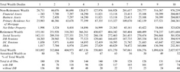
To study the potential distributional consequences of providing annuitization incentives, we consider the wealth distribution of households near the normal retirement age. Table 3.1 replicates a table, based on the Health and Retirement Survey (HRS), from Dushi and Webb (Reference Dushi and Anthony2004). This table consolidates several waves of the HRS to focus on couples for which the head of household is age 65. It provides the wealth distribution by decile for this sample of couples broken down by type of wealth. It excludes the top one percent of the wealth distribution.Footnote 5
Composition of HRS Households' Balance Sheets at Age 65 – Couples

Source: Dushi and Webb (Reference Dushi and Anthony2004) Dushi and Webb (Reference Dushi and Anthony2004).
Notes: Data from Health and Retirement Study, waves 2 to 5. Sample: married couples who turned 65 in any of the waves 2 to 5. Sample size – 1431 observations, from which 13 observations falling in the 100th wealth percentile were dropped resulting in a sample of 1418. We excluded the 100th percentile from the 10th decile and the wealth upper cut-off point is $4,332,141. The present values of Social Security and employer Defined Benefit pensions were calculated using a real rate of interest of 3% and an inflation rate of 2.5%. Annuitized wealth equals the sum of SS and DB pensions. Figures are in 2000 dollars and weighted using household weights. Variation between deciles in number of observations is due to weighting.
Several important patterns emerge from Table 3.1. First, wealth at retirement age is unevenly distributed. The average wealth of the 9th decile is 3.5 times larger than the average wealth of the 2nd decile. In part, this variance highlights the differences across households in how prepared they are for financing retirement. Second, Social Security wealth plays an important role in the balance sheets of these households. Even for the 5th decile, Social Security wealth is almost half (47 percent) of total wealth. Third, defined benefit (DB) pensions account for a substantial fraction of the wealth of this cohort but DB pension wealth is quite unevenly distributed. The combination of Social Security and DB pension wealth implies that many households hold a considerable fraction of their wealth in annuitized forms. The fraction of wealth held in annuitized forms decreases steadily from the bottom decile to the top decile, mainly reflecting the declining importance of Social Security wealth relative to total wealth. Fourth, the amount of wealth in qualified accounts (IRA and DC pensions) is relatively modest for this cohort. However, the data are somewhat dated (based on 1992–2000) so these balances understate the importance of this wealth for current and future cohorts of retirees.
In terms of targeting proposals to increase annuitization, the data in the table suggest that the bottom three deciles of the wealth distribution have little wealth that can be annuitized. Compounding this effect is that much of these groups' wealth outside of Social Security and DB pensions is held as housing equity. Given the common hesitancy for people to move out of their houses and the thinness of reverse mortgage markets, these groups have extremely limited assets available to annuitize. Of course, the table presents averages for the deciles which mask the heterogeneity within the deciles, so many households in these groups may have portfolios that would allow them to benefit from a policy that encourages annuitization.
3.3.3 Cost Effectiveness
The effectiveness of policy proposals depends on the size of the incentives introduced by the policies and how responsive household annuity decisions are to these incentives. The revenue cost to the government depends on several features of the policy, most obviously the effective rate of subsidy and the level at which these benefits are capped. Another key issue is that the treatment of annuities purchased before enactment of the new legislation creates a classic transition concern. If the preferential treatment applies to annuity income from pre-existing annuities as well as income from subsequent annuitization, the legislation will create windfall gains for the owners of pre-enactment annuities and “windfall” revenue losses to the government. It would be cumbersome – and politically inexpedient – to write transition rules to limit these losses. An alternative approach would be to provide a one-time subsidy at the time of annuitization based on the wealth annuitized rather than an annual subsidy based on annuity income. This would allow for similar annuitization incentives but would circumvent cumbersome transition rules (and the political inexpediency). It would, however, involve a substantial front-loading of government revenue costs.
Finally, the level of annuitization that would obtain in the absence of the subsidy policy is also a key input for determining the policy's cost-effectiveness, since subsidization of income from annuities that would have been purchased anyway represents an unavoidable windfall cost.
4 Policy Proposals and the Money's Worth of Currently Available Annuities
The Money's Worth (MW) of an annuity is a measure of how fairly that annuity is priced for a given individual. Specifically, it is the ratio of the expected value of the income stream provided by that annuity to the premium paid for it (see, e.g., Mitchell et al., Reference Mitchell, James, Mark and Jeffrey1999 for details). To compute the Money's Worth of life annuities, we use the mortality tables for the 1920, '30, '40 and '50 cohorts reported in U.S. Social Security Administration's Actuarial Study 120 (Bell and Miller, Reference Bell and Michael2005). We make the plausible assumption that the mortality probabilities of the two annuitants in a joint-and-survivor contract are independent. For convenience, we focus on the couples consisting of a male and a female, each born on the same day of the same year.
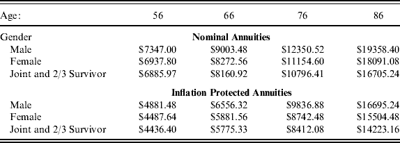
For annuity prices, we use quotes from Vanguard.Footnote 6 They have an online interface that gives instant price quotes for a variety of annuity products. We obtained quotes for men, women and couples living in New York assuming a birthday of July 23rd (since we obtained the data on July 23rd, 2006) for a $100,000 life annuity (without any guaranteed payments) with annual payments starting one year later.Footnote 7 We obtained quotes for nominal and inflation-protected annuities. For joint and survivor annuities, we assumed that the household would want a 2/3 benefit for the surviving spouse regardless of which spouse passes away first.Footnote 8 The price quotes we obtained give the nominal size of the first payment in the income stream. Table 4.1 summarizes these quotes.
Initial payment, per $100,000 premium
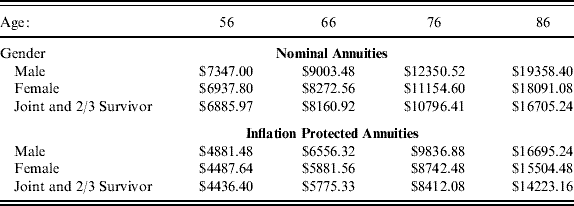
Source: Vanguard.com, 2006. See text for details.
We used the term structure of nominal and inflation protected Treasury bonds as of July 31st, 2006Footnote 9 to determine interest rates and inflation rates. We compute the present value of annuity income streams using the after-tax real interest rate based on this structure and for marginal tax rates mtr=0%, 15%, and 25%. These tax rates also affect the after-tax payments received by annuitants. For qualified annuities, the entire annuity payment is subject to tax, and we take the after-tax payment to be (1 – mtr) of the pre-tax payment. We treat the “cost” of a qualified annuity as (1 – mtr) times the premium paid, since the alternative to annuitizing qualified assets is to withdraw them and subject them to taxation.
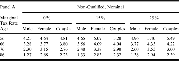
For non-qualified annuities, a portion of the annuity payment is excluded from taxable income as a return of basis. We assume that individuals purchase single-premium immediate non-qualified annuities using a lump sum of cash Y, which we take to be the basis for the annuity purchase (i.e., the cost of the annuity). The tax code recognizes Y/L of each annuity payment as the “return of basis” for each of the first L years, where L is the statutory life expectancy (see IRS Publication 939). A 65 year old male purchasing a nominal life annuity with non-qualified assets would be able to exclude nearly 60% of the payment from his annuity for approximately 15 years, for example.Footnote 10
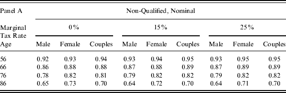
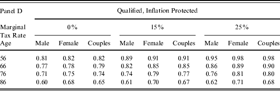
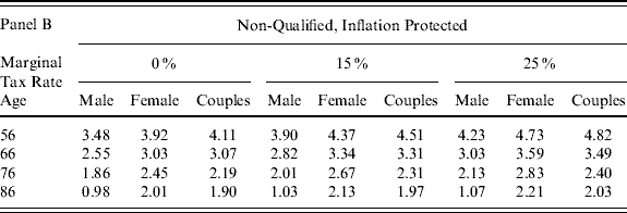
Table 4.2 reports MW's for each of the age and gender groups from Table 4.1 for each of the different tax rates, and for both qualified and non-qualified sources of funds. These MW's indicate that annuity prices are significantly worse than actuarially fair, with insurance loads on the order of 5–10 cents on the dollar for 56 year olds, increasing to 30–35 cents on the dollar for 86 year olds for nominal annuities. These loads are relatively consistent across households of a given age, with males facing slightly higher loads. The age 66 loads are modestly lower than the loads reported by Mitchell et al. (Reference Mitchell, James, Mark and Jeffrey1999), and our results indicate a somewhat steeper increase in loading with age. This sharp increase in loads with age is consistent across products, genders, and tax rates; it is strongly suggestive of an increase in adverse selection loads with age. Consistent with international evidence from James and Vittas (Reference James and Vittas2004), the MWs for inflation protected annuities are uniformly lower than MWs for nominal annuities, implying additional loads of about 6–10 percentage points.Footnote 11
Benchmark Money's Worth Ratios by Gender, Age and Marginal Tax Rates with No Policy Intervention
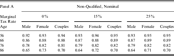
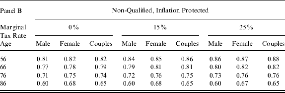
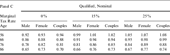
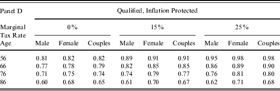
Source: Author's calculations, as described in text. The calculations assume a premium of $100,000. “Couples” refers to a joint-and-survivor annuity for a couple with the same age and a symmetric 2/3 survivor benefit.
Percent Change in Money's Worth Ratios Under Lifetime PAY Bill ($100K Premium)
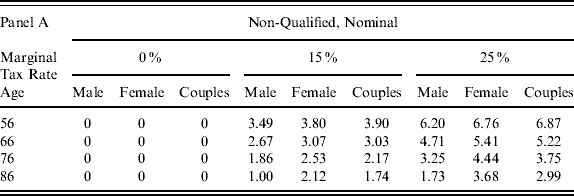
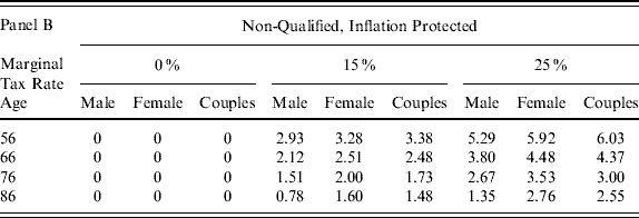
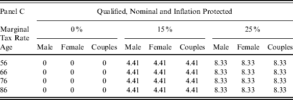
Source: Author's calculations, as described in text. The calculations assume a premium of $100,000. “Couples” refers to a joint-and-survivor annuity for a couple with the same age and a symmetric 2/3 survivor benefit. The entries are the percentage change in the money's worth based on the benchmarks described in Table 4.2.
We next use the MW framework to evaluate the potential effectiveness of policy interventions to enhance annuitization in the U.S. We evaluate the impact of two policy proposals: the tax-exemption based Lifetime PAY bill, H.R. 4150, 110th CongressFootnote 12 and a refundable tax credit policy of comparable magnitude. We model only the direct effect of these policies on the after-tax payments from the annuities in Table 4.1.
The Lifetime PAY bill
The Lifetime PAY bill provides for a tax exemption on 25% or 50% of annuity income, depending on whether the funds used for the purchase are qualified or non-qualified, up to a total of $5,000 in exempted income per person. For households with a positive marginal tax rate, this policy reduces the effective tax rate on annuity income, raising the MW of an annuity by increasing its after-tax real income stream.
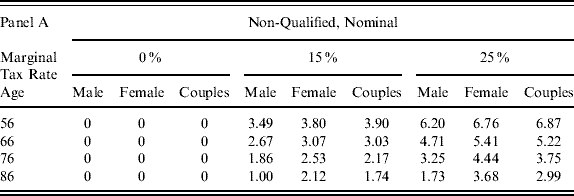
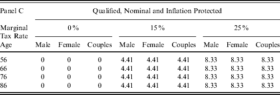
Table 4.3 reports the percentage increases in MWs (over the MWs reported in Table 4.2) for $100,000 annuity policies.Footnote 13Table 4.3 clearly illustrates how the bill most strongly encourages annuitization for annuitants in higher tax brackets (and not at all for households with no tax liability). For non-qualified funds, Table 4.3 indicates that the Lifetime PAY bill has similar MW effects across nominal and inflation protected annuities and across types of households at a given tax rate. The table also illustrates that the bill differentially improves the value of annuitization of non-qualified assets at younger ages relative to at older ages, and it may therefore encourage earlier annuitization.
The effect of the Lifetime PAY bill on the MWs of qualified policies depends on the tax rate but not on the household age or the type of annuity purchased. This is because the $100,000 policy size is small enough to keep annuity income below the limits of the policy, so all payments are subsidized equally. In the 15% tax bracket, for example, each of the annuitant's after tax payments is 4.41% higher – i.e., 100%×{[1 – (.15) (1 – .25)] – (1 – .15))}/(1 – .15), where.15 is the effective marginal tax rate on annuity payments prior to the policy change and (.15) (1 – .25) is the effective marginal tax rate under the policy.
A Tax-Credit Based Policy
Policy proposals such as the Lifetime PAY bill attempt to encourage annuitization at retirement by providing tax exemptions. In this, they parallel the tax advantages provided by most policies designed to encourage retirement savings (e.g., 401(k) accounts). Providing tax exemptions is a natural mechanism for encouraging savings, since the decision to save is distorted by a marginal tax wedge, a distortion well mitigated by an exemption. The case for using exemptions to encourage annuitization is less compelling, since there are no intrinsic tax-rate-based economic distortions. This motivates our decision to analyze a proposal in which the annuitization incentives provided are de-coupled from the marginal tax rate.
Under this policy proposal, the government would provide a 5% refundable tax credit on income from qualified annuities and a 10% refundable tax credit on income from non-qualified annuities, up to a maximum credit of $1,000 per year. These parameters make the tax-credit-policy roughly comparable to the Lifetime PAY proposal. For an individual facing a 20% marginal tax rate, the two policies coincide. For households facing higher marginal tax rates, the Lifetime PAY bill is more generous, and for households facing lower marginal tax rates, the tax-credit policy is more generous. This relative generosity of the two policy interventions is illustrated by comparing Tables 4.3 and Table 4.4, where the latter presents the effects of the tax-credit policy on the MW of $100,000 non-qualified annuity policies. For qualified annuities (assuming the annuity income is below the cap), the effect of the tax-credit is straightforward. For an individual facing no taxes, a 5% subsidy on annuities would increase MW by 5%. The percentage increase in the MW for an individual who faces a positive marginal tax rate is slightly higher since the after-tax value of one dollar inside the account is less than a dollar. For example, for an individual in the 15% tax bracket buying an actuarially fair annuity the MW would increase from 0.85/0.85 (the after-tax present value of annuitizing $1/the after-tax value of $1 withdrawn from a qualified account) to 0.90/0.85, which is a 5.88% increase in the MW.
Percent Change in Money's Worth Ratios Under Tax-Credit Proposal ($100K Premium)
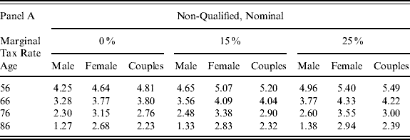
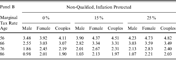
Source: Author's calculations, as described in text. The calculations assume a premium of $100,000. “Couples” refers to a joint-and-survivor annuity for a couple with the same age and a symmetric 2/3 survivor benefit. The entries are the percentage change in the money's worth based on the benchmarks described in Table 4.2.
5 Using Annuity Equivalent Wealth to Evaluate Policy Interventions
5.1 Methodology
The preceding section indicates that tax incentives can increase the monetary value of annuitization. We now use an “Annuity Equivalent Wealth” (AEW) framework to explore the extent to which these price decreases encourage annuitization – in effect, to estimate of the price elasticity of annuitization. The AEW literature typically uses dynamic programming techniques with specific household preferences to compute a monetary value a household would place on annuitizing its entire wealth at actuarially fair rates and at a specified age. (See, e.g., Mitchell et al. (Reference Mitchell, James, Mark and Jeffrey1999) for details.)
More recently, Dushi and Webb (Reference Dushi and Anthony2004) explored the optimal timing of annuitization by measuring the value of annuitizing any amount of wealth at any time using loosely calibrated market prices. While we abstract from timing issues by assuming the annuitization occurs at age 65, our approach allows households' full flexibility in their extent of annuitization, and we use actual market prices. To measure the effect of various policies towards annuitization, we compare the optimal levels of annuitization with and without the policies in place for a distribution of households.
The “annuity puzzle” discussed in Section 2 recommends caution in interpreting the annuitization patterns predicted by the AEW framework. Indeed, our estimates of annuitization levels reflect this puzzle: we “predict” significantly higher annuitization levels than are observed in practice. The usefulness of our estimates lies in the observation that the AEW framework can be a reasonable guide to changes in annuitization patterns even when it over-estimates annuitization levels (viz the discussion in Section 2 and Appendix B).
Our algorithm, discussed in more detail in Appendix A, uses standard household preferences and stochastic mortality to compute the lifetime expected utility, V(W 0, A0), a household anticipates from a given level of (un-annuitized) initial wealth and for a given annuity income stream. For a couple without access to private annuity markets, A0 is the annuity income stream provided by the combination of their Social Security (SS) and defined benefit (DB) pensions. Couples with access to annuity markets can use some of their wealth W 0 to purchase additional annuities, giving them a lower wealth W′0 and a larger annuity stream A′0. Different amounts of annuity purchases will give them different (W′0, A′0) combinations, and hence different lifetime utilities V(W′0, A′0). For computational ease, we assume that annuity markets offer a single type of annuity product, so that there is a one-to-one mapping from annuitization spending W 0− W′0 to the net annuity stream A′0. Our algorithm maximizes V(W′0, A′0) with respect to annuitization spending, thus yielding an optimal amount of annuitization and a lifetime utility V* for the household with access to this annuity product. Our “AEW” then solves:

Equation (5.1) implicitly defines the annuity equivalent wealth as the factor by which initial un-annuitized wealth would need to be increased to compensate the household for removing its access to existing annuity markets. Note that in this formulation, AEW is never less than 1.
The algorithm sketched above is slightly complicated by the presence of two types of wealth – qualified and non-qualified – for a typical retired household (viz Table 3.1). We surmount this complication with two assumptions. First, we assume that households use a stacking rule: they annuitize all of their qualified wealth before annuitizing any of their non-qualified wealth. Qualitatively, the stacking rule seems like a reasonable rule of thumb, since qualified wealth is presumably wealth that households have pre-designated for funding retirement. The evidence appears to corroborate this: Reichenstein (Reference Reichenstein2002) reports that only 2% of individuals who purchase non-qualified deferred annuities ultimately annuitize their balances. In contrast, Johnson et al. (Reference Johnson, Leonard and Deborah2004) report that a larger 10% of individuals with DC plans directly annuitized their assets, and Brown and Warshawsky's (Reference Brown, Mark, Gale, Shoven and Warshawsky2000) report indicating that only 25% of DC plans offered the option to directly annuitize suggests that this may under-estimate ultimate annuitization. However, we emphasize that we impose the stacking rule rather than solving the substantially more difficult dynamic programming problem which would allow individuals the optimal choice of which type of wealth to annuitize. Second, we “tax” any un-annuitized qualified wealth at the household's average tax rate, since households can only consume untaxed portions of any withdrawals.
We start with a collection of 40 households (described below) calibrated to capture the distribution of retired 65 year-old married U.S. households. We consider inflation-protected joint and symmetric 2/3 survivor policies offered by Vanguard as the unique annuitization option available to these households. (We consider similar nominal policies separately.)
To evaluate the effects of a given annuitization-subsidy policy intervention, we solve for each household's optimal amount of annuitized wealth, using the algorithm above, with and without the policy intervention. Comparing annuitization levels in these two regimes gives our estimate of the policy's effect on the annuitization decisions of each household. This procedure effectively amounts to employing AEW techniques to compute annuitization elasticities.
We discussed much of the data required for these calculations – e.g., the mortality tables and the term structures of interest and inflation rates – in Section 4.Footnote 14 For a couple on their 65th birthday, we use an annual payout of $5757.76 and $8108.73 per $100,000 annuitized for inflation protected and nominal annuities, respectively. The remaining inputs consist of preference parameters, tax rates, the size and structure of pre-existing annuities, and the wealth profiles of retired households. We consider these in turn.
Preference parameters: We make standard preference assumptions (see e.g., Brown (Reference Brown2001) or Mitchell et al. (Reference Mitchell, James, Mark and Jeffrey1999)): constant relative risk aversion, additively separable across ages and household members, with discounting of future utility and with consumption complementarities for households with two surviving members. We use a relative risk aversion parameter of 1.5, a “joint consumption factor” of 0.6245 (so that 62.45 cents of each dollar are consumed by both members as in Brown, Reference Brown2001), and a 3% subjective discount rate.
Tax rates: We compute approximate tax rates using the National Bureau of Economics Research's TAXSIM calculator for each of the 40 households (described below). Each household has DB wealth, DC wealth, Social Security wealth, and “other” wealth. For our tax computations, we assume each couple files jointly, has no dependent children, no wages, no dividends, and no special deductions. We take other property income to be 5% of “other” wealth. We assume that taxable pension income is given by 7.5% of pension plus IRA wealth, and that gross Social Security income is given by 7.5% of Social Security wealth. We restrict attention to Federal taxes only by using New Hampshire as the state of residence.
Pre-existing annuities: We treat both Social Security and DB pensions as pre-existing real annuities with 2/3 joint and survivor benefits. The 2/3 survivor benefit is the ratio of the Social Security benefits for a surviving spouse to the Social Security benefits for a couple with one worker with a substantially larger earnings history than the other (e.g., a one earner household).
Households: In constructing a distribution of households, our goal is to consider the wealth distribution of a cohort at the beginning of retirement. We start with the distribution reported by Dushi and Webb (Reference Dushi and Anthony2004) that is summarized in Table 3.1.Footnote 15 To capture heterogeneity within deciles in the levels of pre-annuitized wealth levels and the breakdown of wealth into qualified and non-qualified accounts, we construct four representative households for each decile. Each representative of the decile has the same amount of total wealth (equal to the average total wealth for the decile) but a different composition of wealth. One type of representative from each decile does not have a defined benefit pension so it is defined as having zero DB pension wealth. However, we allocate 80 percent of the decile's overall IRA and DC pension wealth to these couples. The relative weight on this household type (i.e., the fraction of households of this type within the decile) is the fraction of households in the decile that do not report having a DB pension. The other three representative household classes are dubbed “low DB,” “average DB,” and “high DB” households, with relative weights 1:2:1. We compute the DB wealth of the three classes by first distributing all DB wealth for the decile equally across the DB households, and then shifting 50% of the “low DB” households' DB wealth to the “high DB” households. In addition, we allocate each of the DB households a proportional share of the 20 percent of the decile's total IRA and DC pension wealth.Footnote 16 We adjust non-pension financial wealth for each representative to ensure that each has total wealth equal to the decile average.
5.2 Results on Changes in Annuitization and AEWs
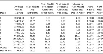
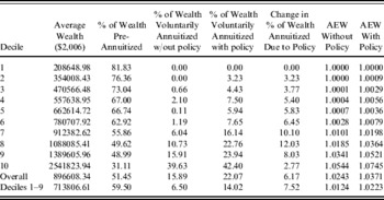
Tables 5.1 and 5.2 summarize our central findings for the effects of the Lifetime PAY bill and our proposed tax-credit policy, respectively, using inflation-protected annuities. In both tables, we present results averaged across the four classes of household within each decile of the population described above. The last two rows present overall or average effects for the entire population and for the subset of the population below the 10th wealth decile, respectively. We present results without the top wealth decile because these households may have bequest motives so that the AEW framework may be less well suited their decisions. Column 4 of both tables reports our estimates of the optimal fraction of wealth voluntarily annuitized in the absence of any policy intervention, and Column 5 contains our estimates of the optimal fractions voluntarily annuitized in the presence of the policy interventions. The next to last row of Column 4 of these tables indicates our estimate that 15.81% of total retirement wealth (6.50% within the first 9 deciles) would be optimally pre-annutized, higher than observed annuitization levels in the HRS (Poterba et al., Reference Poterba, Joshua, Steven and David2003), consistent with the “annuity puzzle” described above. Our annuity puzzle looks even bigger when we use nominal instead of real annuities in our calculations.
Estimated Change in AEW and Annuitized Wealth Induced by Lifetime PAY Bill For Inflation-Protected Annuities

Source: Authors' calculations, as described in text. AEW refers to “Annuity Equivalent Wealth”.
Estimated Change in AEW and Annuitized Wealth Induced by Tax-Credit Policy For Inflation-Protected Annuities

Source: Authors' calculations as described in text. AEW refers to “Annuity Equivalent Wealth”.
Our estimates of changes in the percent of wealth annuitized are reported in Column 6 of the tables. Table 5.1 suggests that the Lifetime PAY bill will increase overall annuitization by 5.67% (6.58% below the 10th decile), an increase of approximately $51,000 of annuitized wealth per household, with the largest percentage increases occurring in the 7th and 8th wealth deciles. Table 5.2 indicates that the tax-credit policy will increase overall annuitization by 6.17% (7.71% below the 10th decile), or about $55,000 per household, with the greatest percentage increases occurring in the same deciles. We obtain similar estimates when we use nominal instead of inflation-protected annuities.
Columns 7 and 8 of Tables 5.1 and 5.2 provide our estimates of the AEW with and without the policy proposals. Since the proposals effectively reduce the load on annuities, they increase the value of having access to these markets, resulting in a higher AEW. For example, the Lifetime PAY proposal increases the AEW for the eighth decile from 1.019 to 1.047. The proposal is thus equivalent to a 2.8% increase in these households' (non pre-annuitized) wealth.
Table 5.1 again confirms what we saw in Section 4: the Lifetime PAY bill is unlikely to have substantial effects in encouraging annuitization among low-wealth households. Column 6 indicates that the annuitization patterns of households in the first four deciles are unaffected by the policy change, and Columns 7 and 8 indicate that their AEW's are unchanged. This simply reflects these households facing marginal tax rates of zero. The tax-credit policy is better targeted towards increasing annuitization among the lower wealth deciles, although even this policy may have no effect for the poorest retired families, whose wealth is mostly pre-annuitized.
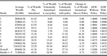
The wealth and pre-annuitization patterns in the populations we constructed from HRS data are reasonable representations of the year 2000 age 65 cohort. To explore the consequences of the trend away from DB wealth and toward DC wealth, we generated a fictional “higher DC-wealth” population by converting 50% of the DB wealth of each of the 40 households in our baseline population to DC wealth. Table 5.3 reports our results on the effectiveness of the Lifetime PAY bill for this population. The estimates in Column 6 indicate that this policy would increase annuitization by 6.10% of retirement wealth, or an average of about $55,000 per household, modestly larger than our previous estimate. The estimates in Table 5.3 differ substantially from Table 5.1 in that they indicate substantially higher baseline (pre-policy) levels of voluntary annuitization – about 27% on average. This reflects the increased importance of voluntary annuitization for households with less pre-annuitized wealth. Estimates for the tax-credit policy show a similar pattern, so we do not present a separate table. We estimate this policy would increase annuitization by about 7.95% on average, or about $71,000 per household.
Estimated Change in AEW and Annuitized Wealth Induced by Lifetime PAY Bill For Inflation-Protected Annuities and For Households with Extra DC Wealth

Source: Authors' calculations as described in text. AEW refers to “Annuity Equivalent Wealth”. “Extra DC wealth” considers the thought experiment of converting ½ of each household's DB pension wealth to DC pension wealth.
While our estimates of changes in annuitization levels are best-guess baseline estimates, there is still considerable uncertainty regarding these estimates.Footnote 17 In particular, they rely on the validity of the AEW framework predicting changes in annuitization patterns in spite of the annuity puzzle, but we feel these predictions are valid under reasonable preference assumptions. As a check on our parameterization of the AEW framework, we calculate the elasticity of demand for annuities implied by the dynamic programming exercise. We compare total predicted annuity demand for our hypothetical distribution of households at market annuity prices with total predicted demand if insurance loads on annuities were one percent lower. This yielded a “load” elasticity of demand of approximately 1.25 for nominal annuities and 3 for inflation-protected annuities. Not surprisingly, given our results that suggest that the policies would substantially increase annuity demand, the dynamic programming approach implies that annuity demand is price elastic.
5.3 Revenue Costs
Our results suggest that both policies would encourage annuitization, but it is important to calculate the revenue costs of these policies. Fixing attention on the age-65 cohort, we focus on the steady-state (per cohort) costs associated with implementing these policies. These costs result from the lower tax rates on annuity income after either policy is implemented. Some of this is the “windfall” cost of subsidizing annuitization that would have taken place anyway.Footnote 18
Our revenue cost estimates are designed to complement the increased annuitization estimates in Column 6 of Tables 5.1, 5.2, and 5.3. For each household, we start with a “baseline” percentage of voluntarily annuitized wealth; we take a range of baselines from a low-end of zero to a high-end taken from the third column of Tables 5.1, 5.2, and 5.3. To each baseline, we then add the sixth-column estimates of the percentage increase in annuitization to obtain a range of estimates for the overall post-policy percentage annuitized for each household. Next, we compute the after-tax real income stream provided by the low-end and high-end post-policy and baseline annuitization levels. Finally, we compute the present discounted value of these after-tax income streams, using the pre-tax real interest rate. The difference between the baseline and the post-policy present values for the low-end and high-end baselines are our low-end and high-end estimates of the revenue cost of the passage of the bill for a household.
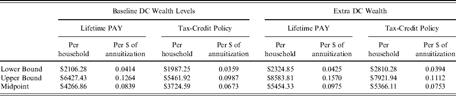
Table 5.4 summarizes our revenue cost estimates for the annuitization levels from Tables 5.1 and 5.2. They suggest that the policies are likely to be cost-effective in the steady-state, with the Lifetime PAY bill (respectively, the tax-credit bill) estimated to cost between about $2,100 and $6,400 per household, or between about 4 and 12 cents per dollar of additional annuitization (respectively, between about $2,000 and $5,500 per household or 3.5 and 10 cents per additional dollar). Similar calculations using nominal annuities raised the lower bound estimates modestly, and approximately doubled the upper bound estimates to about 24 and 18 cents per the dollar for the Lifetime PAY and tax-credit bills, respectively.
Estimated Steady-State Revenue Costs of Policy Interventions
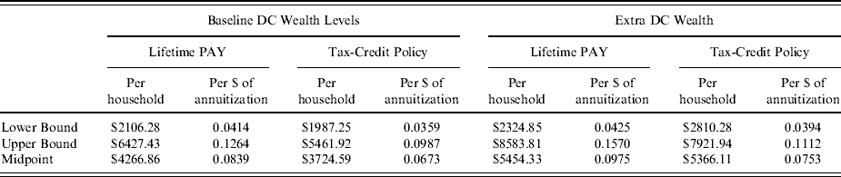
Source: Authors' calculations, as described in text.The left panel reports estimates of the revenue cost of introducing the Lifetime PAY and tax-credit policies on the each cohort as they reach age 65 and annuitize. These are computed by comparing the difference in the present discounted value of a fixed annuity stream with and without the policies. The lower-bound estimates assume zero annuitization prior to the policy implementation, while the upper-bound estimates assume baseline annuitization levels as in the third column of Tables 5.1 and 5.2. the 6th column of Table 5.1 or 5.2. The right panel reports analogous estimates for the fictional population with 50% of each household's DB wealth converted into DC wealth.
Future cohorts will have less of their wealth in defined benefit plans, and therefore will presumably voluntarily annuitize more wealth even without policy interventions. To get a feel for how much this might increase revenue costs, we do analogous calculations using the hypothetical “extra DC wealth” population used in constructing Table 5.3. Table 5.4 also reports these results. It indicates that higher DC balances would indeed increase the costs associated with the policy but that the costs would still remain relatively modest, with upper bounds of about $8,600 and $7,900 per household or about 16 cents and 11 cents per dollar of additional annuitization for the Lifetime PAY policy and tax-credit policies, respectively.
In addition to these steady-state costs, implementing these proposals may create transition costs if older cohorts who have already made their annuitization decisions benefit from the policy change without responding to the policies. One way to avoid these transition costs would be to restrict the policies to transactions that occur after the enactment of the legislation. Even without such a restriction, the windfall gains from these older cohorts benefiting from the policy are likely to be small given the modest levels of actual voluntary annuitization.
6 Conclusions: Policy Options for Encouraging Annuitization
Annuitization decisions of retirees promise to be a growing public policy concern as the baby boom generation retires, life expectancy continues to grow, and the retirement planning landscape continues to shift from traditional pension plans to retirement plans based on personal accounts. The combination of the demographic trends and the change in pension institutions is headed for a confrontation with what economists refer to as the annuity puzzle: households seem reluctant to annuitize their assets voluntarily through private insurance markets, and these markets are much thinner than economic theory predicts they ought to be. While there are many potential causes for the annuity puzzle, public policy can play a role in combating the potential underutilization of these markets.
Our qualitative analysis of the rationales for policy interventions in annuity markets suggests a number of desirable policy features. First, there are economic reasons (apart from potential distributional concerns) for policies to target annuitization incentives towards individuals with low to moderate wealth. The well documented correlation between wealth and longevity implies that such targeted interventions are more effective at addressing adverse selection problems and may therefore be magnified via a “life-spiral.” Additionally, there is a “moral hazard” argument for such targeting: under-annuitization among low-wealth individuals is potentially more costly to a government which serves as an “insurer of last resort” for individuals who exhaust their own resources in old age.
Second, our analysis recommends policies designed to encourage annuitization at earlier ages, when informational asymmetries regarding longevity are likely to be less acute. Third, we observe that an important consideration in designing policy interventions is the fiscal cost. In particular, it may be desirable to design a policy which incentivizes new annuitization while minimizing or avoiding the transition costs associated with incidental benefits provided to households who have already annuitized.
We specifically analyze two possible policy interventions: a tax-exemption based intervention and a refundable tax-credit based intervention. Both policies we consider impose a cap on total annual tax benefits from annuity income. These caps go some way towards targeting benefits at smaller policies purchased by lower-wealth households. Furthermore, these caps actively encourage earlier annuitization among individuals who would exceed the cap were they to annuitize at old age.
Our quantitative analysis of these two policy interventions implies that tax-based proposals could substantially reduce the insurance loads that contribute to households' reluctance to annuitize and could have a substantial effect on the amount of voluntary annuitization in the economy. Our benchmark estimates suggest that 65-year old couples would respond to the policies by increasing the amount of wealth that they annuitize by an average of roughly $50,000. The revenue consequences of these proposals are a concern but, mainly due to the low level of initial annuitization, these proposals appear to have fairly modest revenue costs for the government. We estimate the present value of the steady-state revenue costs to be on the order of 10 cents per additional dollar of annuitized wealth.
While our estimates indicate that the two policies are likely to have similar effects on the overall level of annuitization, we do find significant differences in the distribution of induced increases in annuitization across households of different wealth. Neither policy is particularly effective at encouraging annuitization among the lowest wealth deciles, but the gains from the tax-credit intervention are significantly better targeted towards households with moderate wealth, as compared with the tax-exemption policy whose benefits are disproportionately concentrated in the highest wealth deciles. While we cannot estimate of the magnitude of “life-spiral” and “moral-hazard” reduction benefits of the policy interventions, these considerations clearly recommend the tax credit policy vis-à-vis the tax exemption policy we consider.
Insofar as it would be politically inexpedient to provide tax benefits to income from newly purchased annuities without providing the same benefits to existing annuity streams, neither of the two policies addresses concerns about transition costs. However, it would be possible to provide incentives which are analytically equivalent to those of the tax credit policy via a direct subsidy to new annuity purchases. Such a policy would significantly front-load the revenue costs, however.
Our quantitative analysis is essentially based on the observation that commonly employed “Annuity Equivalent Wealth” techniques can be adapted to provide price elasticity of annuitization estimates. That these techniques have been shown to over-predict empirically observed annuitization levels raises the concern that they may also provide biased elasticity estimates. The literature has not provided precise empirical estimates of how annuitization responds to price incentives, so we cannot empirically corroborate our estimates. The overprediction of annuitization levels provided by this framework should not be taken to indicate that our elasticity estimates will necessarily be biased in any particular direction, however. Indeed, elasticity estimates such as ours can be unbiased even when they significantly overestimate annuitization levels. Furthermore, our methodology omits some important features of the policy that could lead to even larger responses than we predict. First, as annuity markets thicken, one would expect that the private market pricing would improve, especially if adverse selection problems become less severe in these markets. Second, our estimates do not include any “informational responses” to the policy by which a government policy to encourage a behavior plays the role of increasing public awareness of the wisdom of the behavior. Incorporating these effects to refine estimates of the proposals' effects would be a useful but challenging area for further research.
A broader research agenda could explore other mechanisms by which the government might improve annuity markets. Ameriks (Reference Ameriks1999) finds that annuitization rates are quite high for TIAA-CREF participants, typically workers in the education and research sectors. Insofar as these annuitization rates result in part from the substantial financial education about coupling retirement savings with annuitization that TIAA-CREF has traditionally provided, this suggests that financial education and the design of plan rules could also increase annuitization. Of course, TIAA-CREF clients may not be representative of the overall population.
One strategy would focus on financial education for retirement planning. Without entering the business of offering detailed financial advice, the government could potentially provide some general information about retirement options, including the need for savings and the advantages and disadvantages of annuitization. This information could be modeled on the annual statements sent annually to American workers by the Social Security Administration (SSA), statements which explain fairly complicated concepts about annuitization through Social Security.
In terms of redesigning rules, one small step for strengthening the link between retirement savings and annuity markets would be to modify the rules for 401(k) and similar plans to require that life annuities be included as a withdrawal option from these plans. Brown and Warshawsky (Reference Brown and Poterba2000) report that, in 1997, only 27 percent of 401(k) plan participants had the option of purchasing a life annuity without going through a two-step process of withdrawing the funds from the retirement account and rolling them over into an annuity product. Requiring life annuities as a withdrawal option would streamline the annuitization process for many as well as by signaling that the government believes that annuitization is important for retirees. The link between saving and annuitizing through these plans could be made even more explicit in many ways. Following on the behavioral economics findings that the “default” option matters for savings choices through retirement savings plans (Choi et al., Reference Choi, David, Brigitte, Andrew and Wise2004), one could also design these plans such that the default option is that the savings is annuitized at a specific age in the future. Changing the default option would not legally bind anyone to annuitize wealth but would require employees to take an action to avoid annuitization rather than take action to annuitize.
A more stringent approach to linking saving with annuitization would be to redesign 401(k) plans to have two tiers of saving. One tier would work as contributions and withdrawals work under current rules. The other tier would commit the savings to be used as a life annuity. Inducing people to use the second tier could be achieved by offering differentially larger tax incentives for the second tier of savings relative to the first tier.Footnote 19
Appendix A – Formalities of the AEW Calculations
This appendix offers a brief and technical summary of the AEW computation procedure described loosely in Section 5. We break our discussion into three sections. The first describes the preferences of a household and uses them to derive its indirect utility function V(W 0, A) over initial wealth and annuity payment streams. The second section describes how we use this function to derive the AEW of access to a given annuity product. The final section describes how we actually compute the function V(W 0, A).
Throughout this appendix, we assume that all values are real values (i.e., in current dollars) unless we specifically note otherwise.
(i) Preferences
Our AEW procedure involves maximizing the utility of a household with preferences:

where τm and τf are the death age of the male and the female, respectively; P(τm, τf) gives the probability that the male and female will die at ages τm and τf, respectively; where δ=1.03 reflects our assumption that households discount the future by 3% per year; and where
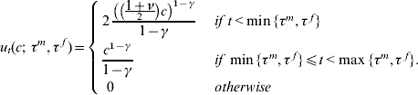
In (A.2), γ=1.5 is the coefficient of relative risk aversion, and ν=.625 measures consumption complementarities if both the husband and wife are living.
The household maximizes its utility over feasible consumption plans of the form:

where the term c t(τm, τf) gives the amount of assets the household plans to consume at age t, if the male and female die at τm and τf, respectively. To capture the fact that the households do not know death ages in advance, we need to impose a feasibility constraint:

Resource constraints also restrict feasible consumptions. Fixing an initial wealth level W 0 and an annuity stream A={(A 65B, …, A 100B), A 65O, …, A 100O}, with the time t annuity payment given by

we impose:

where W t(τm, τf) is defined recursively by W 64(τm, τf)=W 0 and, for 65⩽t⩽100, by:

where r t is the real (annual) after-tax interest rate faced by the household between ages (t – 1) and t. Expression (A.6) reflects our assumption that households cannot borrow against (or sell) their future annuity income. (A.7) reflects our (purely technical) assumption that all wealth is lost once both members of the household have died.
For a given initial wealth an annuity stream, then, the feasible set Γ(W 0, A) of consumption profiles is the set of set of consumption profiles C satisfying (A.4) and (A.6) for all 65⩽t⩽100 and for all 65⩽τm⩽101 and 65⩽τf⩽101.
Finally, we can formally define the lifetime expected utility of a household as a function of an initial wealth and an initial annuity stream:

(ii) Computing AEWs
We assume that there is a single annuity product available for purchase. It is linearly priced: for each $1 premium, it provides a stream of pre-tax life-contingent payments a t(τm, τf). We separately consider two types of annuity, nominal and inflation protected annuities. Nominal annuities pay:

where πt is the ratio of the price levels at age t and age 64. Inflation protected annuities pay:

(A.9) and (A.10) are both joint and 2/3 survivor annuities. Based on Vanguard's pricing, as described in the text, we take a=$8108.73 in (A.9) and a=$5757.76 in (A.10).
Now consider a household with marginal tax rate κ, an average tax rate  , an amount W Q of qualified wealth and an amount W 0 – W Q of non-qualified wealth (with no inside buildup). We use this to compute the real after-tax annuity income function A t*(B, τm, τf). A t*(B, τm, τf) gives the size of the annuity payment at year t for each possible pair of death times for the couple as a function of the amount B the household spends on an annuity. As described in the text, we assume a “stacking rule:” individuals first annuitize their qualified wealth. We separately treat three cases: the baseline case with no policy intervention, the Lifetime Pay policy intervention and the tax-credit policy intervention (viz Section 4.4.2). Following IRS guidelines, we take the de jure life expectancy of a couple to be 22 years, and define the real exclusion amount via:

where we have used the stacking rule and the zero exclusion for qualified annuities.
Case 1: Baseline tax treatment

Equation (A.12) reflects our simplifying “refund of extra basis” assumption discussed in the text (viz Section 4.2.3).
Case 2: Lifetime PAY tax treatment
The Lifetime PAY bill would exempt some annuity income from taxation. Were there no limits, the exemption would be given by:

Equation (A.13) reflects the 25% and 50% exemption for qualified and non-qualified annuity income in the Lifetime PAY bill and our “stacking rule” assumption.
Writing the total exemption, including the $5,000 per living annuitant limit in the bill, we have:

Finally, the after-tax annuity income function is given by:

Case 3: Tax-credit policy intervention
Ignoring limits, the tax-credit intervention we consider provides a refundable tax credit equal to:

Equation (A.16) reflects the 5% and 10% credit on qualified and non-qualified annuity income and our “stacking rule” assumption. Including the $1,000 per live annuitant maximum tax credit, the refundable tax credit is given by:

Finally, the after-tax annuity income function is given by:

Using A*(B) (respectively, A*,LP (B) and A*,S (B)) to denote the entire stream (i.e., the stream for any death date pair) of after tax annuity payments received in exchange for a premium of B under the baseline case (respectively, under the Lifetime PAY bill and the tax-credit policy) we can now describe the household's optimal annuitization decision. Let K(B)=B if B>W Q, and  otherwise (to reflects our assumption that any qualified income which is not annuitized is withdrawn immediately and taxed at the household's average tax rate). Then, under the baseline policy, the household's optimal fraction voluntarily annuitized, αvol* solves:

with obvious analogs for the optimal fractions annuitized, αvol*,LP and αvol*,S in the other two cases. Similarly, we can define the lifetime utility V* for a household with access to a given annuity market in the baseline case (and analogously for the others):

Finally, we implicitly define the AEW of access to a given type of annuity policy via:

(iii) Computing (A.8)
As the first section of this appendix suggests, evaluating the function V(W 0, A) is a non-trivial task. We use standard dynamic program techniques for this. Following Brown (Reference Brown2001) and others, we write the problem in recursive form (i.e., via a Bellman equation). In particular, we define the functions V 100B(W), V 100M(W), and V 100F(W) via:

and then recursively define the value functions for 65⩽t⩽100 via the Bellman equations:

where q tm (respectively, q tf) gives the male (female) mortality rate at age t (i.e., the conditional probability that a male (female) who lives until the last day of his (t – 1)st birthday will die before she reaches his tth birthday).
Finally:

To evaluate (A.24), we discretize the wealth space and approximate the functions V tB(W), V tM(W), and V tF(W) recursively, starting for t=100 by evaluating (A.22), and then numerically optimizing (A.23) via a grid search. This gives us an approximation of (A.24). For a better approximation, we use a finer discretization (in practice, grids with 750 points appear to be sufficient for our purposes).
Finally, we solve (A.20) and (A.21) using a search routine that relies on there being a unique local maximum to that problem; this speeds computation time up significantly relative to a grid search routine.
Appendix B – When is it Valid to Use the AEW framework for “Changes”?
This paper's central estimates hinge on the hope that the AEW framework can provide a good framework for evaluating changes in annuitization patterns even in the presence of the “annuity puzzle” – that is, even when the framework gets the level of annuitization incorrect. This appendix presents a simple class of circumstances under which this hope is borne out and estimates of changes on predicted annuitization levels are exactly correct even though the predicted levels of annuitization are too high.
The AEW framework captures the “value”of annuitization. In appendix A, we focus on the value of having access to an annuity market via the well being of individuals who choose their optimal quantity α* of annuity purchases. This involves determining how well off they would be at any level α of annuitization, and maximizing their well being over all possible values of α. In other words, our estimated levels α* of annuitization maximize some well-being function Z(α). Suppose this well being function takes the following simple form for a single peaked function with maximum at α*:

where k and m are constants.
This model produces an “estimate” of an annuitization level α*, an estimate which may over-estimate empirically observed levels of annuitization. One cause of this over estimate may simply be that the value function captured in (A.25) fails to take into account some decision-relevant “cost” of annuitization – be it a psychological cost, an informational cost, or simply a behavioral artifact attributable to a failure to maximize the “right” thing. If this cost takes a simple linear form, then individuals will behave as if they instead maximize

Consequently, they will choose  and there will be an “annuity puzzle.”
Now consider two policy regimes. Regime s=0 refers to the “no policy” and regime s=1 refers to the “tax-subsidy policy” regime (e.g., under the Lifetime PAY bill). Then we can write

for the “estimated” value function and

for the value function on the basis of which individuals actually make decisions. Our estimates of the increase in annuitization induced by the policy will therefore be α1* – α0*, which will exactly coincide with the actual increase  . In other words, in spite of the annuity puzzle, estimated changes in annuitization rates are a valid guide to actual increases in annuitization rates.
Clearly, this toy example relies on a number of simplifying assumptions which are unlikely to hold exactly in practice. These include the assumptions about the quadratic form of the value function (although this will generically be a good local approximation; the key piece is the assumption that the local curvature of the value function is similar in both policy regimes) and the particular cause of the annuity puzzle (as well as its functional form). Nevertheless, it illustrates that the AEW framework can provide consistent estimates of changes in annuitization even when it gets annuitization levels wrong.
Finally, it is worth noting that, at least in this simplistic model, there can be variability across individuals in the extent of the annuity puzzle (i.e., β can vary across individuals) without affecting the validity of the “changes” estimate.