1. Introduction

The sensitive dependence on initial conditions (SDIC) associated with nonlinear models imposes limitations on the models’ predictive power. These limitations have been widely recognized and extensively discussed.Footnote ¹ In this article we draw attention to an additional problem than has been underappreciated, namely, structural model error (SME). A model has SME if the model dynamics differ from the dynamics in the target system. The central claim of this article is that if a nonlinear model has only the slightest SME, then its ability to generate decision-relevant probabilistic predictions is compromised. We will also show that SME in fact puts us in a worse epistemic situation than SDIC. Given a perfect model, we can take the effects of SDIC into account by substituting probabilistic predictions for point predictions. This route is foreclosed in the case of SME, which relegates both point predictions and accurate probabilistic predictions to the sweet land of idle dreams.

To reach our conclusion, we retell the tale of Laplace’s demon, but with a twist. In our rendering of the tale, the Demon has two apprentices, a Senior Apprentice and a Freshman Apprentice. The abilities of the apprentices fall short of the Demon’s in ways that turn them into explorers of SDIC and SME. By assumption, the Demon can compute the unabridged truth about everything; comparing his predictions with those of the apprentices will reveal the ways in which SDIC and SME curtail our predictive abilities.Footnote ²

In section 2 we introduce our three protagonists as well as basic elements of dynamical systems theory, which provides the theoretical backdrop against which our story is told. In section 3 we follow the apprentices on various adventures that show how predictions break down in the presence of SME. In section 4 we provide a general mathematical argument for our conclusion, thereby defusing worries that the results in section 3 are idiosyncrasies of our example and that they therefore fail to carry over to other nonlinear models. In section 5 we briefly discuss a number of scientific modeling endeavors whose success is threatened by problems with SME, which counters the charge that our analysis of SME is philosophical hairsplitting without scientific relevance. In section 6 we suggest a way of embracing the problem, and in section 7 we draw some general conclusions.

2. The Demon and His Apprentices

Laplace (Reference Laplace1814) invites us to consider a supreme intelligence who is able both to identify all basic components of nature and the forces acting between them and to observe these components’ initial conditions. On the basis of this information, the Demon knows the deterministic equations of motion of the world and uses his unlimited computational power to solve them. The solutions of the equations of motion together with the initial conditions tell him everything he wants to know so that “nothing would be uncertain and the future, as the past, would be present to [his] eyes” (4). This operationally omniscient creature is now known as Laplace’s Demon.

Let us introduce some formal apparatus in order to give a precise statement of the Demon’s capabilities. In order to predict the future, the Demon possesses a mathematical model of the world. It is part of Laplace’s original scenario that the model is a model of the entire world. However, nothing in what follows depends on the model being global in this sense, and so we consider a scenario in which the Demon predicts the behavior of a particular part or aspect of the world. In line with much of the literature on modeling, we refer to this part or aspect of the world as the target system. Mathematically modeling a target system amounts to introducing a dynamical system, , which represents that target system. As indicated by the notation, a dynamical system consists of three elements. The first element, the set , is the system’s state space, which represent states of the target system. The second element, , is a family of functions mapping onto itself, which is known as the time evolution: if the system is in state at time , then it is in at some later time . The state is called the system’s initial condition. In what follows we assume that is deterministic.Footnote ³ For this reason, calculating for some future time and a given initial condition is making a point prediction. In the dynamical systems we are concerned with in this article, the time evolution of a system is generated by the repeated application of a map at discrete time steps: , for ,Footnote ⁴ where is the result of applying U t times. The third element, , is the system’s measure, allowing us to say that parts of X have certain sizes.

With this in place, we can describe Laplace’s Demon as a creature with the following capabilities:

1. 1. Computational Omniscience: he is able to calculate for all and for any arbitrarily fast.

2. 2. Dynamical Omniscience: he is able to formulate the true time evolution of the target system.

3. 3. Observational Omniscience: he is able to determine the true initial condition of the target system.

If these conditions were met, the Demon could compute the future with certainty. Laplace is quick to point out that the human mind “will always remain infinitely removed” from the Demon’s intelligence, of which it offers only a “feeble idea” (Reference Laplace1814, 4). The question then is what these shortcomings are and how they affect our predictive abilities. It is a curious fact that while the failure of computational and observational omniscience has been discussed extensively, relatively little has been said about how not being dynamically omniscient affects our predictive abilities.Footnote ⁵ The aim of this article is to fill this gap.

To aid our explorations, we provide the Demon with two apprentices—the Senior Apprentice and the Freshman Apprentice. Like the master, both apprentices are computationally omniscient. The Demon has shared the gift of dynamical omniscience with the Senior Apprentice: they both have the perfect model. But the Demon has not granted the Senior observational omniscience: she has only noisy observations and can specify the system’s initial condition only within a certain margin of error. The Freshman has not yet been granted either observational or dynamical omniscience: he has neither a perfect model nor precise observations.

Both apprentices are aware of their limitations and come up with coping strategies. They have read Poincaré and Lorenz, and they know that a chaotic system’s time evolution exhibits SDIC: even arbitrarily close initial conditions will follow very different trajectories. This effect, also known as the butterfly effect, makes it misinformative to calculate for an approximate initial condition because even if is arbitrarily close to the true initial condition , and will eventually differ significantly.

To account for their limited knowledge about initial conditions, each apprentice comes up with a probability distribution over relevant initial states, which accounts for their observational uncertainty about the system’s initial condition. Call such a distribution ; the subscript indicates that the distribution describes uncertainty in at .Footnote ⁶ The relevant question then is how initial probabilities change over the course of time. To answer this question, they use to evolve forward in time (i.e., to calculate ). We use square brackets to indicate that is the forward time image of . The time evolution of the distribution is given by the Frobenius-Perron operator (Berger Reference Berger2001, 126–27). If the time evolution is one-to-one, this operator reduces to .

The idea is simple and striking: if provides them with the probability of finding the system’s state at a particular place in at , then is the probability of finding the system’s state at a particular place at any later time . And the apprentices do not only make the (trivial) statement that is a probability distribution in a purely formal sense of being an object that satisfies the mathematical axioms of probability; they are committed to the (nontrivial) claim that the probabilities are decision relevant. In other words, the apprentices take to provide us with predictions about the future of sufficient quality that we ought to place bets, set insurance premiums, or make public policy decisions according to the probabilities given to us by .

This solves the Senior Apprentice’s problem, but the Freshman has a further obstacle to overcome: the fact that his model has a structural model error (SME). We face a SME when the model’s functional form is relevantly different from that of the true system. In technical terms, by SME we mean the condition when the dynamical equations of the model differ from the true equations describing the system under study: in some cases we can write , where is the dynamics of the model, is the true dynamics of the system, and is the difference between the two.Footnote ⁷

The Freshman’s solution to this problem is to adopt what he calls the closeness-to-goodness link. The leading idea behind this link is the maxim that a model that is close enough to the truth will produce predictions that are close enough to what actually happens to be good enough for a certain predictive task. Given that we consider time evolutions that are generated by the iterative application of a map, this idea can be made precise as follows. Let be the Demon’s map (where the subscript T stands for ‘True’, as the Demon has the true model), and let be the Freshman’s approximate time evolution. Then is the difference between the two maps, assuming they share the same state space. Furthermore, let be probabilities obtained under the true time evolution (where ), and the probabilities that result from the approximate time evolution (where ); is the difference between the two. The closeness-to-goodness link says that if is small, then is small too for all times , presupposing an appropriate notion of being small. The notion of being small can be explained in different ways without altering the conclusion. Below we quantify in terms of the maximal one-step error and in terms of the relative entropy of the two distributions.

3. The Apprentices’ Adventures

The Demon schedules a tutorial. The Senior Apprentice claims that while her inability to identify the true initial condition prevents her from making valid point predictions, her probability forecasts are good in the sense that, conditioned on the information the Demon allows her (specifically her initial probability distribution ), she is able to produce a decision-relevant distribution for all later times t. The Freshman does not want to play second fiddle and ventures the bold claim that dynamical omniscience is as unnecessary as observational omniscience and that he can achieve the decision relevance using an imperfect model and the closeness-to-goodness link.

The all-knowing Demon requires them to put their skills to test in a concrete situation in ecology: the evolution over time of a population of rapidly reproducing fish in a pond. To this end, they agree to introduce the population density ratio : the number of fish per cubic meter at time t divided by the maximum number of fish the pond could accommodate per cubic meter. Hence lies in the unit interval . Then they go away and study the situation.

After a while they reconvene and compare notes. The Freshman suggests that the dynamics of the system can be modeled successfully with the well-known logistic map:

where the difference between times and is a generation (which, for ease of presentation, we assume to be 1 week). Recall from section 2 that a dynamical system is a three-partite entity consisting of a state space , a time evolution operator (where if the time evolution is generated by the repeated application of a map at discrete time steps), and a measure . The Freshman’s model is a dynamical system that consists of the state space ; his time evolution is generated by iteratively applying , which is ; is the standard Lebesgue measure on .

The Demon and the Senior Apprentice know the true dynamical law for :

where is a small parameter. The tilde notation is introduced and justified in Smith (Reference Smith2002). The right-hand side of equation (2), which we call the quartic map, is ; applying iteratively yields .

It is immediately clear that the Freshman’s model lacks a small structural perturbation: as the Demon’s map converges toward the Freshman’s. Figure 1 shows both and for , illustrating how small the difference between the two is.

Figure 1.

Equation (1) in blue and equation (2) in yellow, with and on the X-axis and and on the Y-axis.

We now associate the with ’s one-step error: the maximum difference between and for ranging over the entire . The maximum one-step error of the model is at , where and , and hence it is reasonable to say that is small. Applying the closeness-to-goodness link, the Freshman now expects to be small too. That is, starting with the same initial probability distribution , he would expect and to be least broadly similar. We will now see that the Freshman is mistaken.

Since it is impossible to calculate and with pencil and paper, we resort to computer simulation. To this end, we partition into 32 cells, which, in this context, are referred to as bins. These bins are now the atoms of our space for evaluating predictions: in what follows we calculate the probabilities of the system’s state being in a certain bin. This is of course not the same as calculating a continuous probability distribution, but since nothing in what follows hangs on the difference between a continuous distribution and one over bins, and for the sake of notational ease, we refrain from introducing a new variable and take ‘’ and ‘’ to refer to the probabilities of bins. Similarly, a computer cannot handle analytical functions (or real numbers), and so we represent by an ensemble of 1,024 points. We first draw a random initial condition (according to the invariant measure of the logistic map). 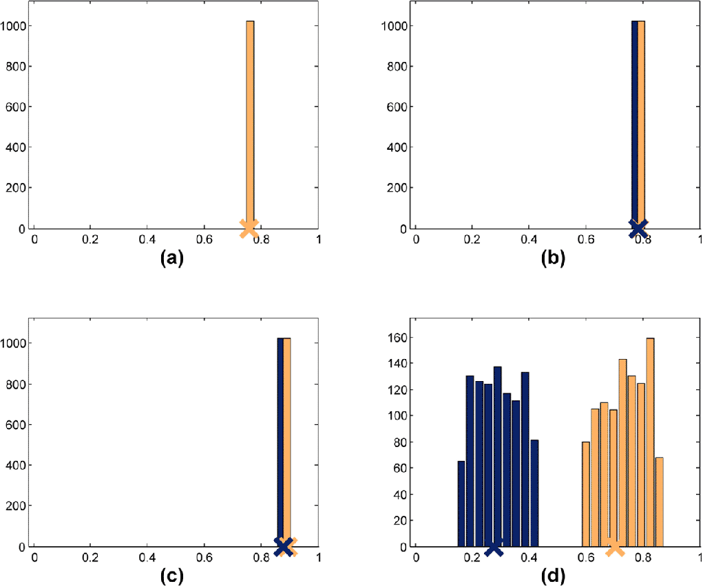By assumption this is the true initial condition of the system at , and it is designated by the cross in figure 2a. We then choose an ensemble of 1,024 points consistent with the true initial condition. These 1,024 points form our ensemble, shown as a distribution in figure 2a. Dividing the numbers on the Y-axis by 1,024 yields an estimate of the probability for the system’s state to be in a particular bin.

Figure 2.

Evolution of the initial probability distribution under the Freshman’s approximate dynamics (blue) and the Senior’s true dynamics (yellow). The yellow cross marks the Demon’s evolution of the true initial condition; the blue cross is the Freshman’s evolution of the true initial condition. Y-axis in d is rescaled to make the details more visible.

We now evolve all these points forward both under the Senior’s dynamics (yellow lines) and the Freshman’s dynamics (blue lines). Figures 2b–2d show how many points there are in each bin at , , and .

While the two distributions overlap relatively well after 2 and 4 weeks, they are almost completely disjoint after 8 weeks. Hence, for this these calculations show the failure of the closeness-to-goodness link: being small does not imply that is also small for all . In fact, for , is as large as can be because there is no overlap at all between the two distributions.Footnote ⁸

Two important points emerge from this example. The first point is that even though chaos undercuts point predictions, one can still make informative probabilistic predictions. The position of the yellow cross is appropriately reflected by the yellow distribution at all times: the yellow probability distribution remains maximally informative about the system’s state given the information available.

The second and more unsettling point is that the ability to reliably make decision-relevant probabilistic forecasts is lost if nonlinearity is combined with SME. Even though the Freshman’s dynamics are very close to the Demon’s, his probabilities are off track: he regards events that do not happen as very likely, while he regards what actually happens as very unlikely. So his predictions here are worse than useless: they are fundamentally misleading. Hence, simply moving an initial distribution forward in time under the dynamics of a model (even a good one) need not yield decision-relevant evidence. Even models that yield deep physical insight can produce disastrous probability forecasts. The fact that a small SME can destroy the utility of a model’s predictions is called the hawkmoth effect.Footnote ⁹ The effect illustrates that the closeness-to-goodness link fails.

This example shows that what truly limits our predictive ability is not SDIC but SME. In other words, it is the hawkmoth effect rather than the butterfly effect that decimates our capability to make decision-relevant forecasts. We can mitigate against the butterfly effect by replacing point forecasts with probabilistic forecasts, but we have no comparable move with force against the hawkmoth effect. And the situation does not change in the long run. It is true that distributions will spread with time and as . As the distribution approaches the system’s natural measure it becomes uninformative. But becoming uninformative and being misleading are very different vices.

One could object that the presentation of our case is biased in various ways. The first alleged bias is the choice of the particular initial distribution shown in figure 2a. This distribution, so the argument goes, has been carefully chosen to drive our point home, but most other distributions would not be misleading in such a way, and our result only shows that unexpected results can occur every now and then but does not amount to a wholesale rejection of the closeness-to-goodness link.

There is of course no denying that the above calculations rely on a particular initial distribution, but that realization does not rehabilitate the closeness-to-goodness link. We have repeated the same calculations with 2,048 different initial distributions (chosen randomly according to the natural measure of the logistic map), and so we obtain 2,048 pairs of and for , , and .

So far we operated with an intuitive notion of the difference between two distributions. But in order to analyze the 2,048 pairs of distributions, we need a formal measure of the difference between two distributions. We choose the so-called relative entropy:

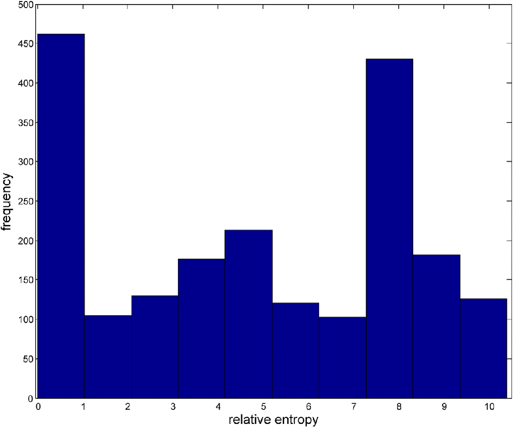
where ‘ln’ is the natural logarithm.Footnote ¹⁰ The relative entropy provides a measure for the overlap of two distributions. If the distributions overlap perfectly— equals —their ratio is then one in the logarithm, and the entropy is zero; the more dissimilar the distributions, the higher the value of . Hence, it is reasonable to consider . Figure 3 shows a histogram of the relative entropy of our 2,048 distributions at .

Figure 3.

Histogram of the relative entropy of 2,048 pairs of distributions at .

The histogram shows that the Freshman’s probabilities are in line with the Senior’s only in about a quarter of the cases. Almost half of the distribution pairs have relative entropy 7 or more. The two distributions shown in figure 2d have a relative entropy of 8.23.Footnote ¹¹ So our histogram shows that at almost half of all distribution pairs are as disconnected as those in figure 2d and, hence, are seriously misleading.

There is a temptation to respond that this does not show that probabilities are useless; it only shows that we should not use these probabilities when they are misleading. The problem with this suggestion is that outside our thought experiment we have no means to tell when that happens. The only thing we have is the model, which we know to be imperfect in various ways. Our tale shows that model probabilities and probabilities in the world can separate dramatically, but we do not know where and when. In cases in which we have no means of separating the good from bad cases,Footnote ¹² we had better be on guard.

The second alleged bias is the use of an 8-week forecast: had we used a different lead time, say 2 or 4 weeks, the Freshman’s endeavors would have been successful because at his distribution is close the Senior’s. Unfortunately this is insufficient: regularly getting the probability distribution only slightly wrong is enough to face catastrophic consequences.

To see this, let us observe the Freshman’s next endeavor. Still not accepting the Demon’s evaluation, he opens the Pond Casino. The Pond Casino functions like a normal casino in that it offers bets at certain odds on certain events, the difference being that the events on which punters can place bets are not outcomes of the spinning of a roulette wheel but future values of . The Freshman takes the above division of the unit interval into 32 bins, which are his basic events (similar to the slots of a roulette wheel), and offers to take bets based on a four-step forecast. More specifically, playing a ‘round’ in the Pond Casino at time amounts to placing a bet at on bin , where the outcome is whether the system is in at . So if you bet, say, on at , you win if is in .

Had the Freshman offered bets on an eight-step forecast, one would expect him to fail given that his probabilities at are fundamentally misleading. Given that his probabilities look close to the Senior’s at , however, he holds the hope that he will do well.

What is the payout for a winning bet? Let be an event that can obtain in whatever game is played in a casino. The odds the casino offers on are the ratio of payout to stake. If, for instance, the casino offers (‘two for one’), a punter who bets £1 on A gets £2 back when obtains. Within the context of standard probability theory, odds are usually taken to be the reciprocals of probabilities: . When flipping an unbiased coin, the probability for heads is 0.5, and if you bet £1 on heads and win, you get £2 back.Footnote ¹³ The Freshman follows this convention and takes the reciprocals of in a four-step forecast as his odds.

Now a group of nine punters enters the casino. Each has £1,000, and they adopt a simple strategy. In every round, the first punter bets 10% of his total wealth on events with probability in the interval . We call this strategy fractional betting (with ) for the probability interval .Footnote ¹⁴ The second punter does the same with events with probability in , the third with events with , and so on, with , , , , , . The minimum bet the casino accepts is £1, so if a punter’s wealth falls below £1 he is effectively broke and has to leave the game.

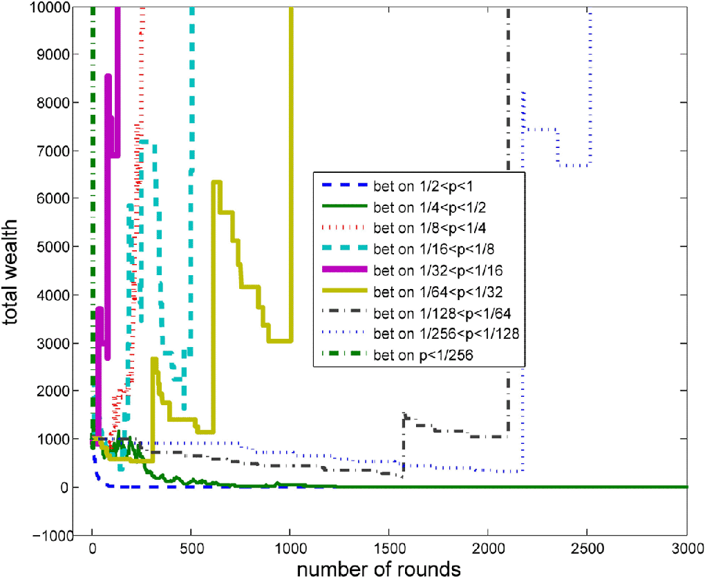
Using the same initial distribution as above (shown in fig. 2a), the Pond Casino now offers odds reflecting the Freshman’s probabilities. The outcomes of bets are of course determined by the true dynamics. We now generate a string of outcomes based on the true dynamics and trace the punters’ wealth, which we display in figure 4 as a function of the number of rounds played.

Figure 4.

Wealth of nine punters as a function of the number of rounds played.

We see that the punters have the time of their lives. Three of them make huge gains very soon, and a further four follow suit a bit later. After 2,500 rounds, seven out of nine punters have increased their wealth at least tenfold, while only two of them have gone bust. So the punters take a huge amount of money off the casino.

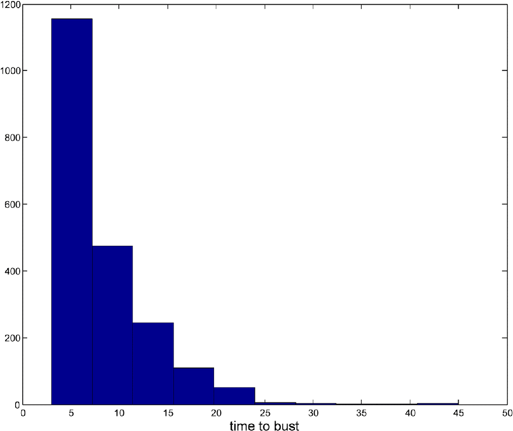
There is a temptation to make the same move as above and argue that this is a ‘bad luck event’ due to the particular initial distribution, which should not be taken as indicative of the casino’s performance in general. We counter in the same vein and consider again 2,048 randomly chosen initial probability distributions. For each of these we let the game take place as before. If the above was a rare special event, then one would expect to see different results in the other 2,047 runs. Since producing another 2,047 plots like the one seen in figure 4 is not a viable way to present the outcomes, we assume that the casino starts with a capital of £1,000,000 and calculate the time to bust. Figure 5 is a histogram of how the casino performs with our 2,048 different initial distributions. Once more the picture is sobering. Most casinos go bust after just a few rounds, and the last one is going out of business after 40 rounds. Offering odds based on is disastrous.

Figure 5.

Histogram of time to bust for 2,048 distributions.

Recall that the punters betting against the apprentice are not using any sophisticated strategy and have no extra knowledge to gain an advantage over the house. They are not, for instance, keeping track of the past as clever punters would (and indeed do in card-counting systems for games like blackjack whereby the bettor exploits the information contained in the past sequence of cards). In such a scenario the bettor is using more informed probabilities than the implied probabilities of the casino’s odds, and it is indeed no surprise if the casino loses money against such bettors.

Our punters are not of this kind. They simply bet on the basis of the values of the odds offered. One punter just bets on all events with implied probabilities in the range . The information is entirely symmetrical—the punters know nothing that the house does not know. Hence, our worry is not just that the apprentice loses money: a punter with access to the system probabilities could obviously do well against the house. Our worry is that the house does disastrously even against punters who know no more than the house.

Frustrated with his failures, the Freshman cannot help himself and starts peeping over the Demon’s shoulder to get the exact initial condition. He convinces the Demon to repeat the entire casino adventure, but rather than moving probability distributions forward in time, he now calculates the trajectory of the true initial condition (which he gleans from the Demon) under his dynamical law. This, he thinks, will guarantee him a success. For want of space we do not follow his further adventures in detail, and in fact there is no need to. A look at figure 2 suffices to realize that he has set himself up for yet another fiasco. The yellow crosses in figure 2 are the true time evolution of the true initial condition; the blue crosses are the Freshman’s time evolution of the true initial condition. We see that the trajectories of the true initial condition under the two dynamical laws soon becomes completely different, and any prediction generated with the model is, once again, seriously misleading. So even if the Freshman was observationally omniscient, he would not be able to generate decision-relevant predictions. SME is a serious issue independently of SDIC. The moral is now unavoidable: offering odds according to the probabilities of an imperfect model can be disastrous even when information is entirely symmetrical between all parties.

4. From Example to Generalization

An obvious line of criticism would be to argue that the problems we describe are specific to the logistic map and do not occur in other systems. So the question is, how general are the effects we have discussed in the last section? To answer this question we review a number of mathematical results about the structural stability of dynamical systems. Our conclusion will be sober. There are special cases in which the above effects do not occur,Footnote ¹⁵ but in general there are no such assurances. Not only are there no general stability results; there are in fact mathematical considerations suggesting that the effects we describe are generic. So we urge a shift of the onus of proof: rather than assuming that nonlinear models are structurally stable and asking the skeptic to make his case, the default assumption ought to be that models are not structurally stable and hence exhibit the effects we describe. Using a particular model for predictive purposes therefore requires an argument to the effect that the model is structurally stable.

Roughly speaking, a dynamical system is structurally stable if its trajectories change only a little if the equation is changed only a little. Andronov and Pontrjagin (Reference Andronov and Pontrjagin1937) presented the first systematic study of structural stability, providing both a definition of structural stability and a theorem. They consider a two-dimensional system that is defined on a disk in the plane with the equations and . We obtain the perturbed system by adding a differentiable function to each equation: and . The original system is structurally stable if and only if for any real number there is a real number such that there exists a smooth -homeomorphism that transforms the trajectories of the original system into trajectories of the perturbed systems. Being an -homeomorphism means that whenever the absolute value of both and as well as their first derivatives are , then the homeomorphism moves each point in by less than .

Given this definition of structural stability, Andronov and Pontrjagin formulate a theorem saying that for a system of the above kind to be structurally stable, it is necessary and sufficient that the following two conditions be satisfied: (i) singularities and closed orbits are hyperbolic, and (ii) there is no trajectory connecting saddle points. However, it turned out that there were problems with their proof. A different proof was given by Peixoto and Peixoto (Reference Peixoto and Peixoto1959).Footnote ¹⁶ Peixoto (Reference Peixoto1962) went on to generalize the result to flows on a compact two-dimensional manifold . He showed that in the space of all differentiable flows on orientable manifolds, structurally stable systems are open and dense in that space relative to the topology. This is often summarized in the slogan that structural stability is generic.

Two-dimensional flows, however, are rather special, which raises the question of what the situation in higher dimensions is.Footnote ¹⁷ While the definition of structural stability carries over swiftly to higher dimensions, generalizing Andronov and Pontrjagin’s theorem to higher dimensional spaces was a formidable problem that turned into a research program spanning almost half a century. The mathematical details cannot be reviewed here; we sketch the main line of argument, which is sufficient for our purposes.

Smale (Reference Smale1967) formulated the so-called Axiom A, which essentially says that the system is uniformly hyperbolic.Footnote ¹⁸ The strong transversality condition says that stable and unstable manifolds must intersect transversely at every point. Palis and Smale (Reference Palis, Smale, Chern and Smale1970) conjectured that a system is structurally stable if and only if it satisfies Axiom A and the strong transversality condition. Proving this result turned out to require a concerted effort and was brought to a conclusion by Mañé (Reference Mañé1988) for diffeomorphisms (‘maps’) and Hayashi (Reference Hayashi1997) for flows.

The relation between structural stability and the Demon scenario is obvious: if the original system is the true dynamics, then the true dynamics has to be structurally stable for the Freshman’s close-by model to yield close-by results. This raises the question whether the systems we are interested in satisfy the above conditions (and hence are structurally stable). This question does not seem to be much discussed, but available results suggest a negative conclusion. Smale (Reference Smale1966) showed that structural stability is not generic in the class of diffeomorphisms on a manifold: the set of structurally stable systems is open but not dense. So there are systems that cannot be approximated by a structurally stable system. More recently, Smith (Reference Smith2002) and Judd and Smith (Reference Judd and Smith2004) presented an argument for the conclusion that if the model’s and the system’s dynamics are not identical, then “no state of the model has a trajectory consistent with observations of the system” (Judd and Smith Reference Judd and Smith2004, 228). Consistency here is defined by the observational noise in the measurements: it quickly becomes clear that there is no model trajectory that could have produced the actual observations; no model trajectory can shadow the measurements (Smith Reference Hagedorn2007). This result holds under very general assumptions.

This has a direct consequence for situations like those considered in sections 2 and 3. If the true dynamics is structurally unstable, then the dynamics of a model with model error (no matter how small) will eventually differ from the true dynamics, resulting in the same initial conditions evolving differently under the two dynamical laws. Given this, we would expect probability distributions like to evolve differently under the two dynamical laws, and we would expect and to have growing relative entropy. We emphasize that these are plausibility assumptions; to the best of our knowledge there are no rigorous proofs of these propositions. Plausibility arguments, however, are better than no arguments at all. And there is certainly no hint of an argument to the effect that high-dimensional systems are structurally stable. So the challenge stands: those using nonlinear models for predictive purposes have to argue that the model they use is one that is structurally stable, and this is not an easy task.

5. Imperfect Models in Action

Our thought experiment has close real-world cousins. In most scientific scenarios the truth is beyond our reach (if such a thing even exists), and we have to rest content with imperfect models—it is a well-rehearsed truism that all models are wrong. Scientists, like the Freshman, are in the situation that they have to produce predictions with a less than perfect model. Some of these predictions are then used to assess the risk of future outcomes. In particular, insurers and policy makers are like the owner of the Pond Casino: they have to set premiums or make policies on the basis of imperfect model outcomes. Examples can be drawn from domains as different as load forecasting in power systems (Fan and Hyndman Reference Fan and Hyndman2012), inventory demand management (Snyder, Ord, and Beaumonta Reference Snyder, Ord and Beaumonta2012), weather forecasting (Hagedorn and Smith Reference Hagedorn and Smith2009), and climate modeling (McGuffie and Henderson-Sellers Reference McGuffie and Henderson-Sellers2005).

But how can nonlinear models be so widely used if their predictive power is as limited as we say it is? Are we overstating the case, or is science embroiled in confusion? The truth, we think, lies somewhere in the middle. The limitations on prediction we draw attention to are debilitating for mathematical precision but not for valuable insight. Hence, at least some scientific projects would need to rethink their methodology in the light of our discussion. A model can be an informative aid to understanding phenomena and processes while at the same time being maladaptive if used for quantitative prediction. As far as we can see, the question of whether the hawkmoth effect threatens certain modeling projects has not yet attracted much attention, and we would encourage those engaged in quantitative prediction in the short run, and even qualitative prediction in the long run, to lend more thought to the matter.Footnote ¹⁹

Another challenge along the same lines argues for the opposite conclusion: if we are interested in long-term behavior, we do not need detailed predictions at all and can just study the natural measure of the dynamics. The natural measure reflects a system’s long-term behavior after the initial distribution ‘washes out’; it is therefore immaterial where we started. It then does not matter that on a medium timescale the distributions look different because we are simply not interested in them.

This view gains support from the fact that we seem to have revealed only half of the truth in section 3. If we continue evolving the distribution forward to higher lead times, we find that for this particular model-system pair the two distributions start looking more similar again and, moreover, that they start looking rather like the natural measure of the logistic map. This is shown in figure 6 for and . Perhaps if all we need is to make reliable predictions in the long run, then the ‘medium term aberrations’ seen in figure 2 need not concern us at all.

Figure 6.

Same scenario as in figure 2 but for lead times (a) and (b) .

Again, while there is similarity in this case, it cannot be expected to happen universally. Implicit in this proposal is the assumption that natural measures of similar dynamical laws are similar—because unless the model and the system have the same natural measures there is no reason to assume that adjusting beliefs according to the natural measure of the model could be informative. While figure 6 is suggestive for this model-system pair (and even this would remain to be shown rigorously), there is every reason to believe that in general natural measures do not have this property. Furthermore, unlike the Demon’s pond, models of many real target systems, such as the world’s climate system, are not stationary and do not have invariant measures at all. This forecloses a response along the above lines. Long-term quantitative prediction is difficult.

How severe the problem is depends on how detailed the predictions one wishes to make are. In general there is a trade-off between precision and feasibility. In the above example it is trivially true that lies between zero and one; we can reliably predict that will not fluctuate outside those bounds (in the model). And there are certainly other general features of the system’s behavior one can gain confidence in with experience. What we cannot predict is that will assume a particular value or will lie in a relatively small area around at a particular point in time, nor can we give probabilities for this to happen. Whether a project runs up against problems with the hawkmoth effect depends on whether it tries to make predictions of the latter kind.Footnote ²⁰

6. A Tentative Suggestion: Sustainable Odds

So far we have discussed problems with imperfect models and pointed out that there is no easy fix. One natural reaction would be to throw in the towel and conclude that the best option would be not to use such models at all. This would be throwing out the baby with the bathwater. Models often show us how things work, and, as we have seen above, in some cases at least a model provides some quantitative insight. So the question is, how can we use the information in a model without being too dramatically misled?

This question has no easy answer because in real science we cannot just peep over the Demon’s shoulder and compare our models with the true dynamics—real scientists are like the Freshman without the Demon (or infinite computer power). So what could the Freshman do to improve his interpretation of model simulations without trying to turn into a Demon (which he cannot)? Failure to grasp this nettle is to pretend he is the Demon. In this section we make a tentative proposal to leave probabilism behind and use nonprobability odds.

As we noted above, the odds on are the ratio of total payout to stake. If there is a probability for , then fair odds on are traditionally taken to be the reciprocals of the probabilities: . This need not be so: we can just as well take odds as our starting point and say that the longer the odds for an event , the more surprising it is if the event occurs. Odds thus understood do not necessarily have any connection to probabilities. Let be a complete set of events,Footnote ²¹ let , , be the odds on all the events in , and define . They are probability odds only if ; they are nonprobability odds otherwise.Footnote ²² Furthermore, let us call the betting quotients on . The are ‘probability-like’ in that they are numbers between zero and one, with one indicating that the obtaining of an event is no surprise at all and zero representing a complete surprise.

With this in place, let us continue our thought experiment. The Freshman wants to try to run a casino without going bust. From his last experience he knows that using probability odds set according to appears a recipe for disaster. So he decides to shorten his odds to guard against loss. Of course you can always guard against loss by not paying out any net gain at all and merely returning the stake to punters when they win (i.e., by setting all ). This, however, is not interesting to punters, and they would not play in his new casino. So the Freshman aims to offer a game that is as attractive as possible, by offering odds that are as long as possible, but only so long that he is unlikely to go bust unexpectedly.

There are different ways of shortening odds. Perhaps the simplest way is to impose a threshold on the : if , and if , where can be any real number so that . We call odds thus calculated threshold odds. For the limiting case of the correspond to probabilities, and the respective odds correspond to probabilistic odds. It is important to emphasize that the threshold rule applies to all possible events and not only the atoms of the partition—the idea being that one simply does not offer ’s smaller than no matter what the event under consideration is. In particular, the rule applies simultaneously to events and their negation. If, for instance, we set and have (and hence, by the axioms of probability, ), then and , where is the negation of (i.e., the nonoccurrence of ).

This move is motivated by the following observation. In figure 2 we see that, based on , we sometimes offer very long odds on events that are in reality (i.e., according to ) very likely to happen. It is with these events that we run up huge losses. Putting a lower bound on the amounts to limiting large odds and thus the amount one pays out for an actual event that one’s model wrongly regarded as unlikely.

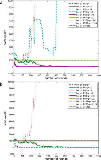
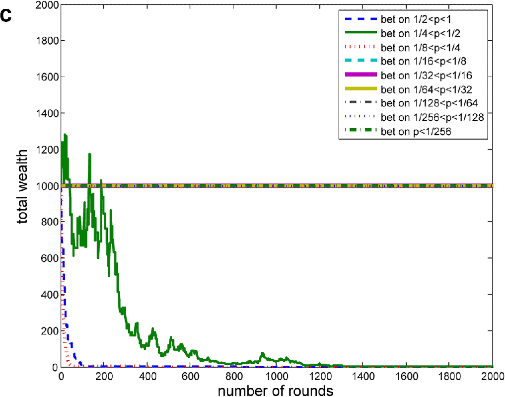
We now repeat the scenario of figure 4 with one exception: the Freshman Apprentice now offers nonprobability odds with a thresholds of , , and . The result of these calculations is shown in figures 7a, 7b, and 7c, respectively.

Figure 7.

Wealth of punters as a function of the number of rounds played with the casino offering threshold odds, with thresholds of (a) 0.05, (b) 0.1, and (c) 0.2.

We see that this strategy brings some success. Already a very low threshold of undercuts the success of five out of seven punters, and only two still manage to take money off the casino. A slightly higher threshold of brings the number of successful punters down to one. So for the Freshman Apprentice achieves his goal of running a sustainable casino.

The second way of shortening odds is damping. On this method the betting quotients are given by , where the damping parameter is a real number . We see that for the correspond to probabilities. We call odds thus calculated damping odds. We now repeat the same calculations as above, and the results are very similar (which is why we are not reproducing the graphs here). For only two punters succeed (indeed the same two as above). With a slightly stronger damping of only one is still winning (again the same as above), and for all punters are either losing or not playing at all (because no bets in their range are on offer).

The moral of this last part of our tale is that shortening odds, either by introducing a threshold or by damping, can provide some protection against losses. In doing so the Freshman has attempted to introduce what we call sustainable odds. There are no doubt better ways to construct sustainable odds and better meet the challenges to their use in decision support. How to construct more useful varieties of sustainable odds is the question for a future project. For now we just note that while probability odds are easier to use, using them leads to disaster. Furthermore, we can regard the amount of deviation of the shortening parameters from their ‘probability limits’ (i.e., the deviation of from zero and of from one) as a measure of the model inadequacy: the greater this deviation, the less adequate the model.

We would like to point out that also this last part is closer to reality than it seems. The sustainable yet interesting casino is modeled on a cooperative insurance company. Rather than playing for gain, the ‘bets’ placed are insurance policies bought to compensate for losses suffered should certain events happen. What makes our insurance a cooperative insurance is its attempt to offer a full payout (to fully compensate its clients) at the lowest rates that allow it to operate in a sustainable way (an insurance company that goes bust is of little use). So our nonprobability odds casino has a close real-world cousin, and the morals drawn above are relevant beyond the tale of Laplace’s Demon.

So far we have shown that one is all but certain to go bust when allowing bets on model probabilities. The conclusion of our argument might be seen as a decision-theoretic one: that it is pragmatically advantageous to adopt nonprobabilistic odds. This is not the interpretation we favor. We prefer to see it as an epistemological argument, albeit one that involves talk of betting. We are not making any decision-theoretic assumptions in coming to our conclusions. We mean for our agent to be shortening his odds due to epistemological flaws, not just so as to avoid bad outcomes. Talk of casinos, betting, and going bust helps to put an epistemic problem into focus—the main point is that the pragmatic flaw (systematic and statistically premature ruin) points to an epistemological flaw in the agent’s representation of belief.

Needless to say, the use of nonprobability odds raises a host of issues. How exactly should nonprobability odds inform decision making? Presented with nonprobability odds, what decision rules should we apply? These are important questions for decision theory and rational choice, but we cannot discuss these here.

An attempt to dismiss these issues quickly might be to try to bring these issues back into well-charted territory by denying that nonprobability odds are really sui generis items. Regarding them as such, so the argument goes, is a red herring because, even if we have odds whose inverses do not add up to one, it is trivial to renormalize them, and we then retrieve the homely probabilities for which there are well-worked-out decision theories.

Unfortunately things are not as simple. The problem is that the do not satisfy the axioms of probability even if they are renormalized to add up to one. The source of the problem is that nonprobability odds do not respect the symmetry between betting for and betting against that is enshrined into probabilities. For probabilities, we have for any event .Footnote ²³ Nonprobability odds need not add up to one: can take any value greater than one (which is easy to see in the case of threshold odds). For this reason the are not probabilities, and renormalizing is not an easy route back into the well-charted territory of probabilism. And, of course, the renormalized odds need not prove sustainable.

Furthermore, one might worry that these nonprobabilistic odds do not have the requisite connection to degrees of belief in order for them to play the role of fixing degrees of belief. That is, one might worry that such odds allow one to avoid the pragmatically bad consequences of model error, but they do not line up with degrees of belief. For example, Williamson (Reference Williamson2010) argues that symmetry—the claim that your limiting price to sell a bet should be equal to your limiting price to buy that bet—is an intuitive part of what he calls the ‘betting interpretation’ of degrees of belief: “While we do in, practice, buy and sell bets at different rates, the rate at which we would be prepared to both buy and sell, if we had to, remains a plausible interpretation of strength of belief” (37). Others disagree and do suggest that nonsymmetrical odds can serve as a (perhaps partial) characterization of strength of belief (see, e.g., Dempster Reference Dempster1961; Good Reference Good, Nagel, Suppes and Tarski1962; Levi Reference Levi1974; Suppes Reference Suppes1974; Kyburg Reference Kyburg1978; Walley Reference Walley1991; Bradley Reference Bradley, Dieks, Gonzalez, Hartmann, Stoeltzner and Weber2012). If one knows one’s model is imperfect, it is hard to see a successful case in favor of symmetrical odds from model-based probabilities as relevant to rational belief or action.

We would not like to leave the issue without a brief remark about Dutch books. One might worry that our Freshman is subject to a Dutch book when he offers nonprobabilistic odds. That is, one might worry that a smarter bettor might be able to guarantee to make money out of the apprentice by buying a set of bets that guarantee the bettor a sure gain, whatever happens. This is not the case. This is for the same reason that casinos cannot be Dutch booked. In a casino, you cannot bet on ‘not red’ with symmetrical probability to ‘red’.

In connection with this point, it is worth pointing out an analogy between the current project and the standard Dutch book argument. The latter argues from a pragmatic flaw (being subject to a Dutch book) to an epistemic conclusion (your degrees of belief ought to satisfy the probability calculus). We take ourselves to be doing the same sort of thing: we argue from a pragmatic flaw (houses go bust faster than expected, statistically) to an epistemic conclusion (nonprobability odds). That is, we do not take ourselves to be merely making the point that one can avoid going bankrupt by shortening one’s odds. We are making the stronger claim that in the presence of model error, model probabilities sanction only nonprobability degrees of belief.

We conclude this section with an explanation of why one final response to our argument will not succeed. One might respond that we get wrong probabilities because we use probabilities in a bad way. From a Bayesian perspective one could point out that by using one particular model to generate predictions we have implicitly assigned a prior probability of 1 to that model. Given that we have no reason to assume that this model is true—indeed, there are good reasons to assume that it is not—this confidence is misplaced, and one really ought to take uncertainty about the model into account. This can be done by using probabilities: put a probability measure on the space of all models that expresses our uncertainty about the true model, generate predictions with all those models, and take some kind of weighted aggregate of the result. This, so the argument goes, would avoid the above problem, which is rooted in completely ignoring second-order uncertainty about models.

Setting aside the fact that it is unfeasible to generate predictions with an entire class of models, in practice there are theoretical limitations that ground the project. The first problem is that it is not clear how to circumscribe the relevant model class. This class would contain all possible models of a target system. But the phrase ‘all models’ masks the fact that mathematically this class is not defined, and indeed it is not clear whether it is definable at all. The second problem is that even if one could construct such a class in one way or another, there are both technical and conceptual problems with putting an uncertainty measure over this class. The technical problem is that the relevant class of models would be a class of functions, and function spaces do not come equipped with measures. In fact, it is not clear how to put a measure on function spaces.Footnote ²⁴ The conceptual issue is that even if the technical problem could be circumvented somehow, what measure would we chose? The model class will contain an infinity of models, and it is at best unclear whether there is a nonarbitrary measure on such a set that reflects our uncertainty about model choice. And even if one can form a revised probability distribution in light of higher-order doubt about the model, it will still be inaccurate relative to the distribution given by the true model.Footnote ²⁵ Finally, we, like the Freshman, are restricted to sampling from the set of all conceivable models, which need not contain a perfect model even if such a thing exists. For these reasons this response does not seem to be workable.

7. Conclusion

We have argued that model imperfection in the presence of nonlinear dynamics is a poison pill: treating model outputs as probability predictions can be seriously misleading. Many operational probability forecasts are therefore unreliable as a guide to rational action if interpreted as providing the probability of various outcomes. Yet not all the models underlying these forecasts are useless.

This raises the question, what conclusion we are to draw from the insight into the unreliability of models? An extreme reaction would be to simply get rid of them. But this would probably amount to throwing out the baby with the bathwater because imperfect models can be qualitatively informative. Restricting models to tasks of purely qualitative understanding is also going too far. The question is how we can use the model where it provides insight while guarding against damage where it does not. Finding a way of doing this is a challenge for future research. We have indicated that one possible route could be to use nonprobability odds, but more needs to be said about how these can be used to provide decision support, and there may be altogether different ways of avoiding the difficulties we sketch. We hope this article leads merely to a wider acknowledgment that these challenges are important and their solution nontrivial.