1 Introduction
Buoyant jets and plumes are found in a variety of natural and engineering contexts, including industrial burners (Christopher et al. Reference Christopher, Wimer, Lapointe, Hayden, Grooms, Rieker and Hamlington2018; Hayden et al. Reference Hayden, Petrykowski, Sanchez, Nigam, Lapointe, Christopher, Wimer, Upadhye, Strobel and Hamlington2019), hydrothermal vents (Gaskin & Wood Reference Gaskin and Wood2001) and volcanic plumes (Campion et al. Reference Campion, Delgado-Granados, Legrand, Taquet, Boulesteix, Pedraza-Espitía and Lecocq2018). Despite their obvious differences, each of these flows exhibit a similar ‘puffing’ phenomenon that results from the continuous injection of less dense fluid into a reservoir of more dense, ambient fluid. The associated fluxes of momentum and buoyancy through the inlet lead to the formation of vortical structures that are periodically shed, yielding the puffing behaviour. The resulting puffing frequency,  $f$, can be characterized using the Strouhal number,
 $St_{\ell }=f\ell /V_{0}$, and the balance between momentum and buoyancy inlet fluxes is typically characterized by the Richardson number,
 $Ri_{\ell }=(1-\unicode[STIX]{x1D70C}_{0}/\unicode[STIX]{x1D70C}_{\infty })g\ell /V_{0}^{2}$, where
 $\ell$ and
 $V_{0}$ are, respectively, the characteristic dimension and inlet velocity of the flow,
 $\unicode[STIX]{x1D70C}_{0}$ is the density of the inlet fluid,
 $\unicode[STIX]{x1D70C}_{\infty }$ is the ambient density and
 $g$ is the gravitational acceleration. Typically, buoyant jets are classified as those flows where
 $Ri_{\ell }<1$ and momentum flux is dominant, at least in the near field, while buoyant plumes are dominated by buoyancy fluxes and have
 $Ri_{\ell }>1$ (Bharadwaj & Das Reference Bharadwaj and Das2017).
Puffing of buoyant jets and plumes has been examined in detail over the past three decades, beginning with Hamins, Yang & Kashiwagi (Reference Hamins, Yang and Kashiwagi1992) and Cetegen & Kasper (Reference Cetegen and Kasper1996). In both of these studies, round helium buoyant jets and plumes were studied over a range of Richardson and Reynolds,  $Re_{\ell }=V_{0}\ell /\unicode[STIX]{x1D708}_{0}$, numbers, where
 $\unicode[STIX]{x1D708}_{0}$ is the kinematic velocity of the inlet fluid. Hamins et al. (Reference Hamins, Yang and Kashiwagi1992) found that the Strouhal and Richardson numbers were related as
 $St_{D}\sim Ri_{D}^{0.38}$, where
 $D$ is the inlet diameter. Cetegen & Kasper (Reference Cetegen and Kasper1996) similarly determined the relation
 $St_{D}=0.8Ri_{D}^{0.38}$ for
 $Ri_{D}<100$ and
 $St_{D}=2.1Ri_{D}^{0.28}$ for
 $100<Ri_{D}<500$. In a study of planar (i.e., high aspect ratio rectangular) buoyant jets and plumes, Cetegen, Dong & Soteriou (Reference Cetegen, Dong and Soteriou1998) found the alternative relation
 $St_{W}=0.55Ri_{W}^{0.45}$, where
 $W$ is the inlet width. The differences in round and planar scaling relations were attributed to differences in mixing rates and buoyancy fluxes between the different inlet shapes. Additionally, the puffing Strouhal number was found to be independent of Reynolds number (Cetegen Reference Cetegen1997).
More recently, Bharadwaj & Das (Reference Bharadwaj and Das2017) performed a comprehensive study of round helium buoyant plumes using global linear stability analysis, as well as experiments in both orifice and pipe-nozzle configurations. Least square fits to the experimental data yielded scaling relations  $St_{D}=0.78Ri_{D}^{0.39}$ and
 $St_{D}=0.82Ri_{D}^{0.38}$ for the orifice and pipe-nozzle configurations, respectively, both of which were in good agreement with the relation
 $St_{D}=0.82Ri_{D}^{0.39}$ obtained for the primary puffing mode from global linear stability analysis. Interestingly, the stability analysis revealed the presence of a secondary puffing mode, which was also captured experimentally, with a transition in the frequencies of the primary and secondary modes at
 $Ri_{D}\approx 6000$; up to this critical Richardson number, the primary mode had the smaller puffing frequency, and above this number the second mode had the smaller frequency. A similar global stability analysis for round thermal (i.e., high temperature) buoyant jets and plumes by Chakravarthy, Lesshafft & Huerre (Reference Chakravarthy, Lesshafft and Huerre2018) provided a slightly larger scaling exponent of
 $St_{D}\propto Ri_{D}^{0.43}$ for the primary mode; the difference between this result and that from Bharadwaj & Das (Reference Bharadwaj and Das2017) was attributed to the different sources of buoyancy (i.e., helium inflow versus high-temperature gases) in the two stability analyses.
Although these various prior scaling relations are useful when studying round or planar buoyant jets and plumes, they are not directly applicable to inlets of different shapes. This can pose challenges in many practical applications involving complex inlets (e.g., industrial burners or volcanic plumes). Recently, Bharadwaj & Das (Reference Bharadwaj and Das2019) experimentally studied a series of buoyant jets and plumes created by helium inflow from rectangular inlets with different aspect ratios and found that all puffing Strouhal numbers could be described using a single Richardson number scaling relation when the characteristic length,  $\ell$, was taken to be the hydraulic diameter of the inlet, and the characteristic velocity was taken to be the effective velocity of a jet with the same total mass flow rate issuing through a round exit with a diameter equal to the hydraulic diameter. The question remains, however, whether a single scaling relation based on the hydraulic diameter (or radius) can be used to relate Strouhal and Richardson numbers for a wider range of inlet geometries, including the rectangular inlets with different aspect ratios studied by Bharadwaj & Das (Reference Bharadwaj and Das2019).
In the present study, we take the first steps towards determining whether such a relation exists by using adaptive mesh numerical simulations to examine high-temperature buoyant jets and plumes for circular, rectangular (with three different aspect ratios), triangular and annular inlet geometries. A range of Richardson numbers are examined for each geometry, and we show that a single scaling relation based on the hydraulic radius accurately describes all available experimental and computational data for hydraulic Richardson numbers spanning roughly four orders of magnitude. It should be noted that the highest Richardson numbers achieved in the present simulations are of the order of  $10^{2}$, restricting the analysis to the primary instability mode identified by Bharadwaj & Das (Reference Bharadwaj and Das2017). Fully resolved simulations of much higher Richardson numbers at and above the transition between secondary and primary modes remain the subject of future research, and require substantially greater computational resources (e.g., to increase the size of the inlet).
2 Description of adaptive mesh numerical simulations
2.1 Numerical configuration
The numerical code used to perform the adaptive mesh simulations is PeleLM, a low-Mach reacting flow code (Almgren et al. Reference Almgren, Bell, Colella, Howell and Welcome1998; Day & Bell Reference Day and Bell2000; Bell et al. Reference Bell, Day, Shepherd, Johnson, Cheng, Grcar, Beckner and Lijewski2005; Nonaka et al. Reference Nonaka, Bell, Day, Gilet, Almgren and Minion2012; Nonaka, Day & Bell Reference Nonaka, Day and Bell2018) that solves a low-Mach formulation of the Navier–Stokes equations, as well as additional equations for enthalpy and species conservation. These equations are summarized for the present non-reacting simulations as (Nonaka et al. Reference Nonaka, Day and Bell2018)
 $$\begin{eqnarray}\displaystyle & \displaystyle \frac{\unicode[STIX]{x2202}u_{i}}{\unicode[STIX]{x2202}t}+u_{j}\frac{\unicode[STIX]{x2202}u_{i}}{\unicode[STIX]{x2202}x_{j}}=-\frac{1}{\unicode[STIX]{x1D70C}}\frac{\unicode[STIX]{x2202}\unicode[STIX]{x03C0}}{\unicode[STIX]{x2202}x_{i}}+g_{i}+\frac{1}{\unicode[STIX]{x1D70C}}\frac{\unicode[STIX]{x2202}}{\unicode[STIX]{x2202}x_{j}}\left[\unicode[STIX]{x1D707}\left(\frac{\unicode[STIX]{x2202}u_{i}}{\unicode[STIX]{x2202}x_{j}}+\frac{\unicode[STIX]{x2202}u_{j}}{\unicode[STIX]{x2202}x_{i}}-\frac{2}{3}\unicode[STIX]{x1D6FF}_{ij}\frac{\unicode[STIX]{x2202}u_{k}}{\unicode[STIX]{x2202}x_{k}}\right)\right], & \displaystyle\end{eqnarray}$$
 $$\begin{eqnarray}\displaystyle & \displaystyle \frac{\unicode[STIX]{x2202}(\unicode[STIX]{x1D70C}Y_{\unicode[STIX]{x1D6FC}})}{\unicode[STIX]{x2202}t}+\frac{\unicode[STIX]{x2202}(u_{j}\unicode[STIX]{x1D70C}Y_{\unicode[STIX]{x1D6FC}})}{\unicode[STIX]{x2202}x_{j}}=\frac{\unicode[STIX]{x2202}\unicode[STIX]{x1D6E4}_{\unicode[STIX]{x1D6FC}j}}{\unicode[STIX]{x2202}x_{j}}, & \displaystyle\end{eqnarray}$$
 $$\begin{eqnarray}\displaystyle & \displaystyle \frac{\unicode[STIX]{x2202}(\unicode[STIX]{x1D70C}h)}{\unicode[STIX]{x2202}t}+\frac{\unicode[STIX]{x2202}(u_{j}\unicode[STIX]{x1D70C}h)}{\unicode[STIX]{x2202}x_{j}}=\frac{\unicode[STIX]{x2202}}{\unicode[STIX]{x2202}x_{j}}\left(\unicode[STIX]{x1D706}\frac{\unicode[STIX]{x2202}T}{\unicode[STIX]{x2202}x_{j}}\right)+\frac{\unicode[STIX]{x2202}}{\unicode[STIX]{x2202}x_{j}}\left(\mathop{\sum }_{\unicode[STIX]{x1D6FC}}h_{\unicode[STIX]{x1D6FC}}\unicode[STIX]{x1D6E4}_{\unicode[STIX]{x1D6FC}j}\right), & \displaystyle\end{eqnarray}$$
where  $u_{i}$ is the velocity,
 $\unicode[STIX]{x1D70C}$ is the density,
 $g_{i}$ is the gravitational acceleration vector,
 $Y_{\unicode[STIX]{x1D6FC}}$ is the mass fraction of species
 $\unicode[STIX]{x1D6FC}$ and
 $h$ is the sensible enthalpy. Due to the low-Mach formulation, only the pressure perturbation field
 $\unicode[STIX]{x03C0}(\boldsymbol{x},t)$ appears in (2.1). This field is combined with the background pressure
 $p_{0}$ to give the total pressure
 $p(\boldsymbol{x},t)$ as
 $$\begin{eqnarray}p(\boldsymbol{x},t)=p_{0}+\unicode[STIX]{x03C0}(\boldsymbol{x},t).\end{eqnarray}$$
Key to the low-Mach formulation is the assumption that  $\unicode[STIX]{x03C0}/p_{0}$ depends on Mach number,
 $M$, as
 $O(M^{2})$, and that
 $M$ is small. Using the ideal gas equation of state,
 $p_{0}$ is related to
 $\unicode[STIX]{x1D70C}$ and the temperature,
 $T$, as
 $$\begin{eqnarray}p_{0}=\unicode[STIX]{x1D70C}{\mathcal{R}}T\mathop{\sum }_{\unicode[STIX]{x1D6FC}}\frac{Y_{\unicode[STIX]{x1D6FC}}}{W_{\unicode[STIX]{x1D6FC}}},\end{eqnarray}$$
where  ${\mathcal{R}}$ is the universal gas constant and
 $W_{\unicode[STIX]{x1D6FC}}$ is the molecular weight of species
 $\unicode[STIX]{x1D6FC}$.
The perturbation field  $\unicode[STIX]{x03C0}(\boldsymbol{x},t)$ is determined by imposing the divergence constraint (Nonaka et al. Reference Nonaka, Day and Bell2018)
 $$\begin{eqnarray}\frac{\unicode[STIX]{x2202}u_{i}}{\unicode[STIX]{x2202}x_{i}}=\frac{1}{\unicode[STIX]{x1D70C}c_{p}T}\left[\frac{\unicode[STIX]{x2202}}{\unicode[STIX]{x2202}x_{j}}\left(\unicode[STIX]{x1D706}\frac{\unicode[STIX]{x2202}T}{\unicode[STIX]{x2202}x_{j}}\right)+\frac{\unicode[STIX]{x2202}}{\unicode[STIX]{x2202}x_{j}}\left(\mathop{\sum }_{\unicode[STIX]{x1D6FC}}h_{\unicode[STIX]{x1D6FC}}\unicode[STIX]{x1D6E4}_{\unicode[STIX]{x1D6FC}j}\right)\right]+\frac{1}{\unicode[STIX]{x1D70C}}\mathop{\sum }_{\unicode[STIX]{x1D6FC}}\left(\frac{W_{mix}}{W_{\unicode[STIX]{x1D6FC}}}-\frac{h_{\unicode[STIX]{x1D6FC}}}{c_{p}T}\right)\frac{\unicode[STIX]{x2202}\unicode[STIX]{x1D6E4}_{\unicode[STIX]{x1D6FC}j}}{\unicode[STIX]{x2202}x_{j}},\end{eqnarray}$$
where  $c_{p}=c_{p}(T)$ is the specific heat capacity at constant pressure. As outlined by Nonaka et al. (Reference Nonaka, Day and Bell2018), this constraint is obtained from a combination of the continuity equation describing conservation of mass, namely
 $$\begin{eqnarray}\frac{\unicode[STIX]{x2202}\unicode[STIX]{x1D70C}}{\unicode[STIX]{x2202}t}+\frac{\unicode[STIX]{x2202}(u_{j}\unicode[STIX]{x1D70C})}{\unicode[STIX]{x2202}x_{j}}=0,\end{eqnarray}$$
as well as the transport equations for  $Y_{\unicode[STIX]{x1D6FC}}$ and
 $h$ in (2.2) and (2.3), respectively.
All fluid transport properties are calculated as mixture-averaged coefficients assuming a mixture of perfect gases. The viscosity,  $\unicode[STIX]{x1D707}$, and thermal diffusivity,
 $\unicode[STIX]{x1D706}$, depend on
 $T$ and
 $Y_{\unicode[STIX]{x1D6FC}}$, and the mass diffusivity of species
 $\unicode[STIX]{x1D6FC}$, namely
 $D_{\unicode[STIX]{x1D6FC}}$, depends only on
 $T$. The enthalpy of species
 $\unicode[STIX]{x1D6FC}$, namely
 $h_{\unicode[STIX]{x1D6FC}}$, also depends only on
 $T$ and the total sensible enthalpy is obtained as
 $h=\sum _{\unicode[STIX]{x1D6FC}}Y_{\unicode[STIX]{x1D6FC}}h_{\unicode[STIX]{x1D6FC}}$. The mixture-averaged molecular weight,
 $W_{mix}$, is given by
 $W_{mix}=(\sum _{\unicode[STIX]{x1D6FC}}Y_{\unicode[STIX]{x1D6FC}}/W_{\unicode[STIX]{x1D6FC}})^{-1}$. Finally, the diffusive flux
 $\unicode[STIX]{x1D6E4}_{\unicode[STIX]{x1D6FC}j}$ in (2.2) and (2.3) is given by
 $$\begin{eqnarray}\unicode[STIX]{x1D6E4}_{\unicode[STIX]{x1D6FC}j}=\unicode[STIX]{x1D70C}D_{\unicode[STIX]{x1D6FC}}\frac{W_{mix}}{W_{\unicode[STIX]{x1D6FC}}}\frac{\unicode[STIX]{x2202}Y_{\unicode[STIX]{x1D6FC}}}{\unicode[STIX]{x2202}x_{j}},\end{eqnarray}$$
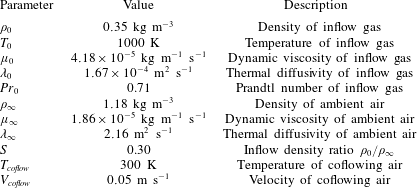
where summation over repeated Greek indices is not implied. A summary of the transport coefficients used in the present simulations is provided in table 1.
Fluid properties and boundary conditions held constant across all simulations.

The simulations were performed in a  $1~\text{m}^{3}$ domain using adaptive mesh refinement (AMR) to reduce the computational cost. The adaptive grid approach implemented in PeleLM is described in detail by Day & Bell (Reference Day and Bell2000), and the governing equations were solved on a series of uniform, nested grids with no subgrid-scale (SGS) modelling. A second-order Godunov scheme is used for advection and a semi-implicit discretization is used for diffusion. The overall numerical method is second-order accurate in both space and time, and the time step is dynamically determined according to an advective Courant–Friedrichs–Levy condition. A more comprehensive description of the numerical approach, algorithm and methods is available in Nonaka et al. (Reference Nonaka, Day and Bell2018) and Wimer et al. (Reference Wimer, Day, Lapointe, Makowiecki, Glusman, Daily, Rieker and Hamlington2019).
The computational domain for each simulation consisted of a  $128\times 128\times 128$ base grid with two levels of AMR. The grid was remeshed every time step to maintain sufficiently fine resolution in regions with large vorticity and density gradient magnitudes, and to reduce resolution in regions where magnitudes were small. With two levels of AMR, the smallest physical scale resolved in the simulations was 1.95 mm, which was recently shown to be sufficiently fine for accurate resolution of the puffing frequency of a large-scale helium plume using an identical numerical approach and similar physical set-up (Wimer et al. Reference Wimer, Day, Lapointe, Makowiecki, Glusman, Daily, Rieker and Hamlington2019). A description of grid convergence in the present simulations is also provided here in § 2.3.
2.2 Physical configuration
The bottom boundary in each of the simulations consisted of a high temperature inlet and a mild air coflow. Open boundary conditions were used on the four sides and at the top of the domain. The inlet and coflow were specified using Dirichlet boundary conditions, and the open boundaries were specified using a divergence-constrained velocity projection that allowed for both fluid inflow and outflow. In each of the simulations, hot air with temperature  $T_{0}=1000$ K flowed from the inlet, and the inlet velocity,
 $V_{0}$, was varied to span a range of Richardson numbers (see table 2). The coflow was uniform and the same in all simulations, with velocity
 $V_{coflow}=0.05~\text{m}~\text{s}^{-1}$ and temperature
 $T_{coflow}=300$ K. The gravitational acceleration was directed downwards with magnitude
 $g=9.81~\text{m}~\text{s}^{-2}$ towards the bottom boundary along the vertical axis. A summary of inlet conditions held constant across all simulations is provided in table 1.
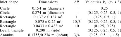
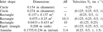
Summary of simulations performed, indicating the shape of the inlet, its dimensions and aspect ratio,  $AR$, and the inlet velocities,
 $V_{0}$, examined for each shape. In all simulations, the inlet temperature was
 $T_{0}=1000$ K and the
 $1~\text{m}^{3}$ domain was discretized with a
 $128\times 128\times 128$ base grid and two levels of AMR, providing an effective grid resolution of 1.95 mm.
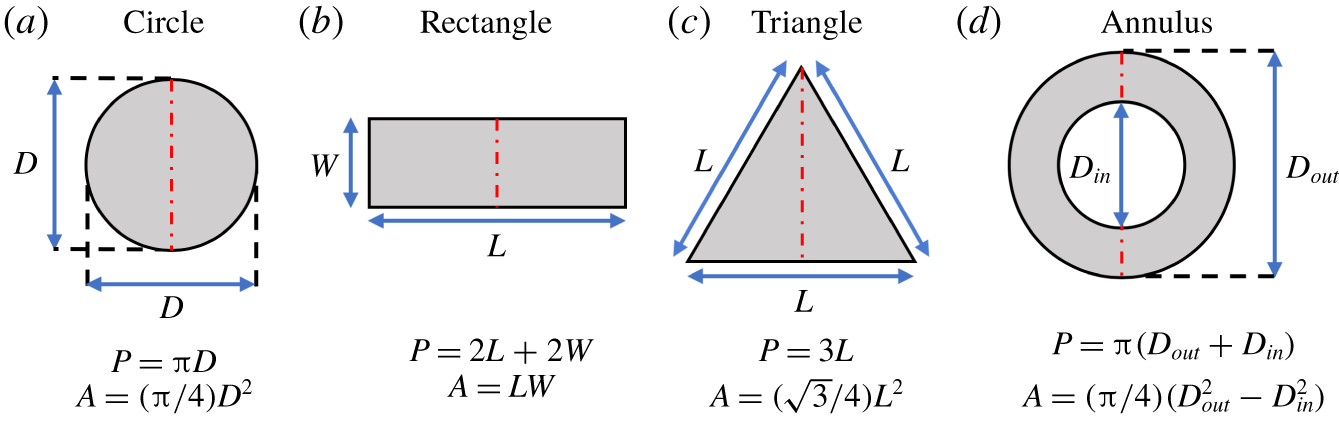
Schematics of the inlet shapes examined in the present study, including formulae for the area  $A$ and perimeter
 $P$ of each shape used to compute the hydraulic radius
 $R_{h}=A/P$. The red dash-dot lines indicate the directions along which the two-dimensional fields discussed in §§ 2.3 and 3.2 are shown.

Seven different inlet shapes were simulated (summarized in table 2 and shown schematically in figure 1): circles with two different diameters; rectangles with three different aspect ratios; an equilateral triangle; and an annulus. The aspect ratios of the rectangles are computed as  $AR_{rect}=L/W$, where
 $L$ is the length and
 $W$ is the width, with
 $L>W$ and
 $1\leqslant AR_{rect}<\infty$. Three rectangular aspect ratios were considered here, corresponding to
 $AR_{rect}=1,10/3,10$. The aspect ratio for the annulus is given by
 $AR_{annu}=D_{in}/D_{out}$, where
 $D_{in}$ is the inner diameter and
 $D_{out}$ is the outer diameter, with
 $D_{in}<D_{out}$ and
 $0\leqslant AR_{annu}<1$. An annulus of aspect ratio,
 $AR_{annu}=3/4$ was examined here. Each of the simulations were performed for 20 s and statistics were computed over the last 10 s to allow for the decay of initial transients.
Taken together, the configurations summarized in table 2 span roughly three orders of magnitude in Richardson number. To condense the description of these configurations, and given the different definitions of Richardson number used herein, we simply refer to each of these flows as ‘buoyant jets’. The primary methods by which the Richardson number can be further increased, thereby allowing the study of the secondary puffing mode identified by Bharadwaj & Das (Reference Bharadwaj and Das2017), are by increasing the size of the inlet, or by reducing the inlet velocity. The former, however, necessitates larger computational domains, while the latter causes the flow to develop more slowly, thereby requiring longer simulation times. Lower inlet velocities may also lead to numerical difficulties, since the inlet velocity begins to rival the diffusion velocity of the helium source, which is not explicitly modelled in the present simulations. As a result, the study of larger Richardson numbers and, in particular, the secondary puffing mode identified by Bharadwaj & Das (Reference Bharadwaj and Das2017) are left as important directions for future research.
2.3 Grid convergence
The governing equations outlined in § 2.1 are solved on a series of uniform, nested grids without an SGS model. Since there is no explicit SGS model, dissipation of kinetic energy is achieved in the simulations through a combination of numerical and physical dissipation, where the former is connected to the second-order numerical scheme used in PeleLM and the latter arises from viscous stresses in (2.1). When the simulation resolution is coarse, numerical dissipation of kinetic energy can be large, or even dominant, compared to the physical dissipation provided by viscous stresses. As the simulation resolution improves, however, the magnitude of numerical dissipation becomes progressively smaller, until physical dissipation is the dominant remaining mechanism of kinetic energy dissipation. In such cases, further improvements in the resolution will result in negligible changes to the simulation results, and the simulations can thus be considered grid-converged.
It should be noted that the present simulations, even though lacking an explicit SGS model, are not implicit large eddy simulations (ILES). In the case of ILES, there is often no physical viscosity term in the governing equations (see, e.g., the governing equations solved in the numerical studies by Benzi et al. (Reference Benzi, Biferale, Fisher, Kadanoff, Lamb and Toschi2008) and Hamlington, Poludnenko & Oran (Reference Hamlington, Poludnenko and Oran2011)), and all kinetic energy dissipation is accomplished numerically. Due to the presence of a physical viscosity term, by contrast, the present simulation approach is more appropriately considered under-resolved direct numerical simulation (DNS) at coarse resolutions, and true DNS at finer resolutions.
Although attempts have been made to quantify the magnitude of numerical dissipation relative to physical dissipation (e.g., by Benzi et al. (Reference Benzi, Biferale, Fisher, Kadanoff, Lamb and Toschi2008)), here we consider quantities of primary interest in the simulations and seek a grid resolution for which these quantities do not substantially change upon further refinements of the grid. In the present study, our primary interest is in the near-field flow structure and dynamics of buoyant jets and plumes, and we correspondingly examine the convergence of velocity and temperature statistics up to second order, as well as the convergence of the puffing frequency, in simulations of a circular buoyant jet with progressively finer physical resolutions. Convergence of AMR simulations using a nearly identical numerical and physical configuration in PeleLM has also been performed by Wimer et al. (Reference Wimer, Day, Lapointe, Makowiecki, Glusman, Daily, Rieker and Hamlington2019) for a large-scale helium plume, yielding a similar convergence criterion to that found here.
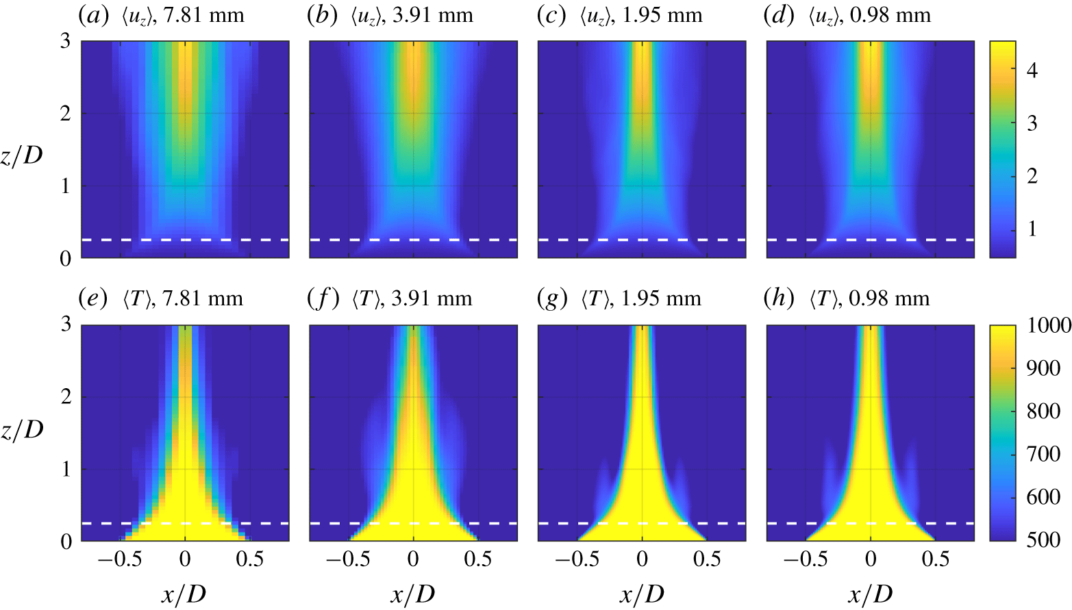
Two-dimensional fields of the time-averaged vertical velocity  $\langle u_{z}\rangle$ in
 $\text{m}~\text{s}^{-1}$ (a–d) and the time-averaged temperature
 $\langle T\rangle$ in K (e–h) for a circular buoyant jet with
 $D=0.154$ m,
 $T_{0}=1000$ K and
 $V_{0}=0.5~\text{m}~\text{s}^{-1}$ at simulation resolutions of 7.81 mm (a,e), 3.91 mm (b,f), 1.95 mm (c,g) and 0.98 mm (d,h). The horizontal dashed lines indicate the height of the transverse profiles at
 $z/D=0.25$ in figure 3.

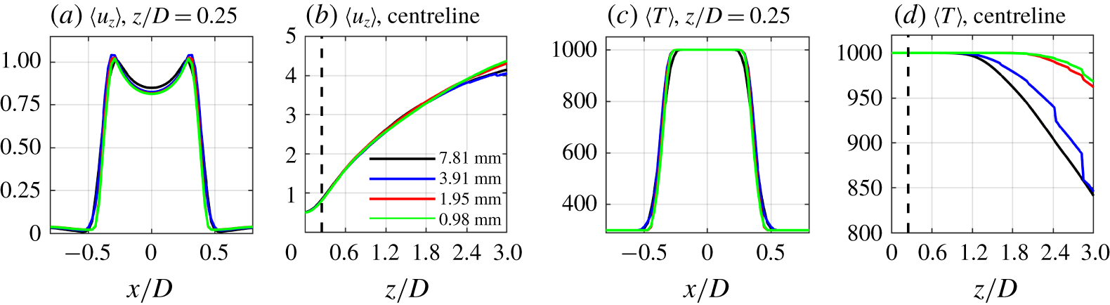
Transverse (a,c) and centreline (b,d) profiles of the time-averaged vertical velocity  $\langle u_{z}\rangle$ in
 $\text{m}~\text{s}^{-1}$ (a,b) and the time-averaged temperature
 $\langle T\rangle$ in K (c,d) for a circular buoyant jet with
 $D=0.154$ m,
 $T_{0}=1000$ K and
 $V_{0}=0.5~\text{m}~\text{s}^{-1}$ at simulation resolutions of 7.81 mm, 3.91 mm, 1.95 mm and 0.98 mm. The vertical dashed lines in panels (b,c) indicate the location of the transverse profiles at
 $z/D=0.25$ in panels (a,c), and all profiles have been interpolated to uniform grids.

We perform four simulations of circular buoyant jets with identical initial and boundary conditions, but with different fine-scale resolutions of 7.81 mm, 3.91 mm, 1.95 mm and 0.98 mm, corresponding to zero through three levels of AMR. The diameter of the circular plumes is  $D=0.154$ m, with inlet conditions
 $T_{0}=1000$ K and
 $V_{0}=0.5~\text{m}~\text{s}^{-1}$. The approximate computational cost of the four simulations presented are 700 processor hours (cpu hours) for the 7.81 mm resolution, 5000 cpu hours for the 3.91 mm resolution, 13 000 cpu hours for the 1.95 mm resolution, and 50 000 cpu hours for the 0.98 mm resolution.
Figure 2 shows two-dimensional (2-D) time-averaged fields of the vertical velocity  $u_{z}$ and the temperature
 $T$, where the time average, denoted
 $\langle \cdot \rangle$, is taken over a 10 s period after the simulations have been running for 10 s. The fields of
 $\langle u_{z}\rangle$ and
 $\langle T\rangle$ are qualitatively similar for each of the resolutions, in particular showing an increase in the vertical velocity above the inlet due to buoyancy and an inward ‘necking’ of the high-temperature region. Specific details of the flow are also quantitatively similar for the two finest resolutions, as indicated by the transverse and centreline profiles of
 $\langle u_{z}\rangle$ and
 $\langle T\rangle$ shown in figure 3. The transverse profiles in figures 3(a) and (c) are taken at the same height as the calculations of the puffing frequency presented later in this study, corresponding to
 $z/D=0.25$, and show that
 $\langle u_{z}\rangle$ and
 $\langle T\rangle$ are in good agreement for resolutions of 1.95 mm and 0.98 mm. The centreline profiles in figures 3(b) and (d) show similarly good agreement between the two finest resolutions.
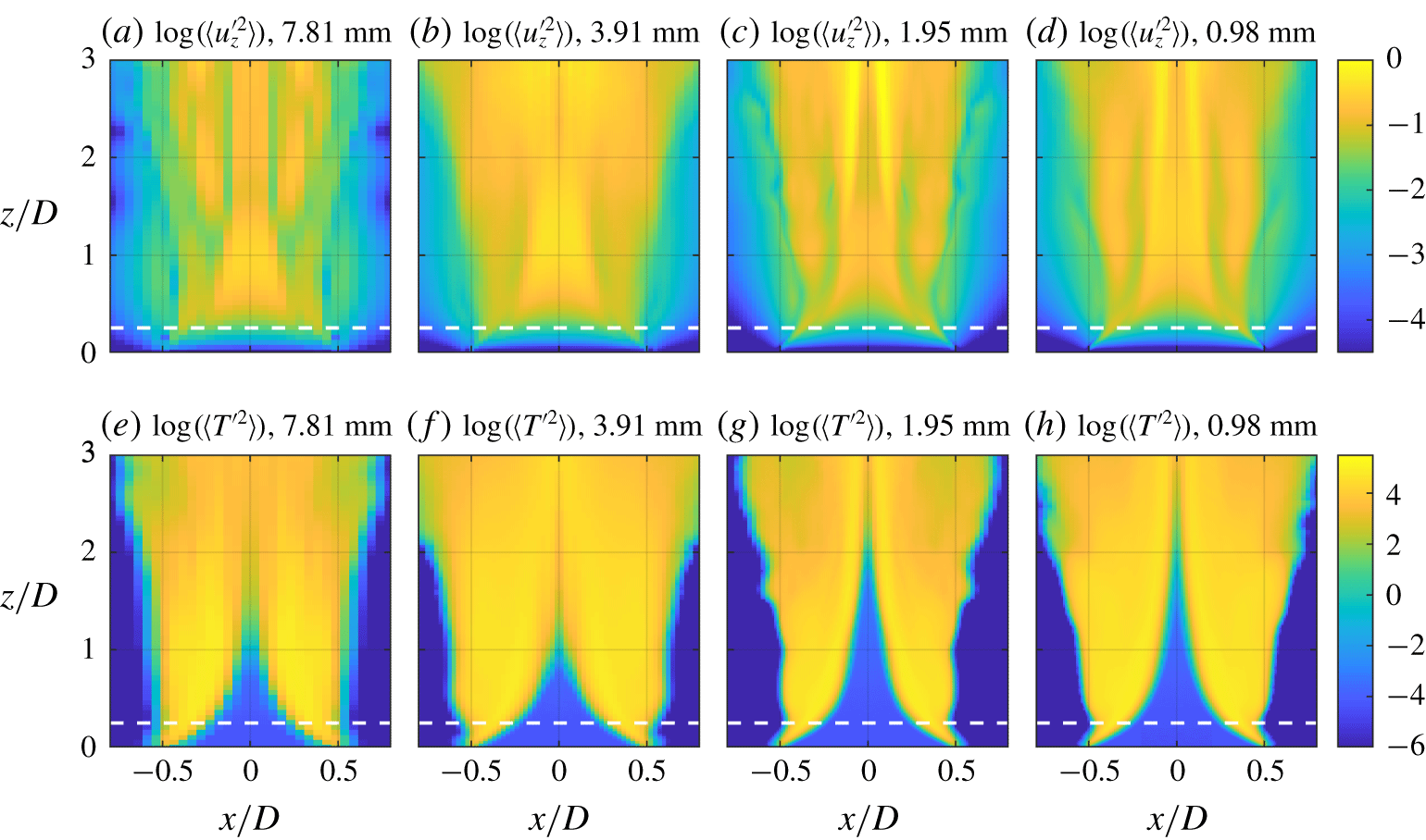
Two-dimensional fields of the time-averaged vertical velocity variance  $\langle u_{z}^{\prime 2}\rangle$ in
 $\text{m}^{2}~\text{s}^{-2}$ (a–d) and the time-averaged temperature variance
 $\langle T^{\prime 2}\rangle$ in
 $\text{K}^{2}$ (e–h) for a circular buoyant jet with
 $D=0.154$ m,
 $T_{0}=1000$ K and
 $V_{0}=0.5~\text{m}~\text{s}^{-1}$ at simulation resolutions of 7.81 mm (a,e), 3.91 mm (b,f), 1.95 mm (c,g) and 0.98 mm (d,h). The horizontal dashed lines indicate the height of the transverse profiles at
 $z/D=0.25$ in figure 5.

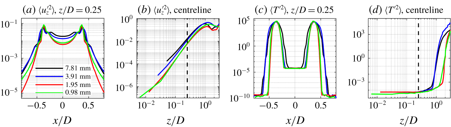
Transverse (a,c) and centreline (b,d) profiles of the time-averaged vertical velocity variance  $\langle u_{z}^{\prime 2}\rangle$ in
 $\text{m}^{2}~\text{s}^{-2}$ (a,b) and the time-averaged temperature variance
 $\langle T^{\prime 2}\rangle$ in
 $\text{K}^{2}$ (c,d) for a circular buoyant jet with
 $D=0.154$ m,
 $T_{0}=1000$ K and
 $V_{0}=0.5~\text{m}~\text{s}^{-1}$ at simulation resolutions of 7.81 mm, 3.91 mm, 1.95 mm and 0.98 mm. The vertical dashed lines in panels (b,c) indicate the location of the transverse profiles at
 $z/D=0.25$ in panels (a,c), and all profiles have been interpolated to uniform grids.

In general, resolution requirements in flow simulations become more strict as the statistical order of the quantity of interest increases, and figure 4 shows 2-D fields of the variances  $\langle u_{z}^{\prime 2}\rangle$ and
 $\langle T^{\prime 2}\rangle$. Compared to the first-order averages in figure 2, figure 4 shows that there are larger changes in
 $\langle u_{z}^{\prime 2}\rangle$ and
 $\langle T^{\prime 2}\rangle$ as the resolution increases. In particular, the spatial variations in
 $\langle u_{z}^{\prime 2}\rangle$ for the finest resolution (0.98 mm) are only captured by the next coarsest resolution (1.95 mm). Similarly,
 $\langle T^{\prime 2}\rangle$ remains small along the centreline up to two diameters above the inlet for the finest simulation, but this feature is not captured for resolutions coarser than 1.95 mm. The transverse and centreline profiles of
 $\langle u_{z}^{\prime 2}\rangle$ and
 $\langle T^{\prime 2}\rangle$ in figure 5 also depend more sensitively on resolution than the first-order profiles in figure 3, now showing that resolutions coarser than 1.95 mm fail to capture the profiles obtained for the finest resolution. The only substantial differences between the two finest resolution cases are in
 $\langle u_{z}^{\prime 2}\rangle$ near the edges of the inlet, as shown in figure 5(a), but the values of
 $\langle u_{z}^{\prime 2}\rangle$ in this region are roughly four orders of magnitude smaller than the peak values and the differences in the profiles are consequently of less concern.
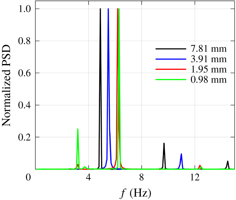
Power spectral densities, PSD, of the vertical velocity for three different resolution simulations of a circular buoyant plume with  $D=0.154$ m,
 $V_{0}=0.5~\text{m}~\text{s}^{-1}$ and
 $T_{0}=1000$ K. The frequencies corresponding to the peaks in the PSD for each of the simulations are 4.90 Hz (resolution of 7.81 mm), 5.49 Hz (resolution of 3.91 mm), 6.19 Hz (resolution of 1.95 mm) and 6.29 Hz (resolution of 0.98 mm).

With respect to the quantity of primary interest in this study – the puffing frequency – figure 6 shows the power spectral density (PSD) of the vertical component of velocity taken half a diameter above the inlet. The peak puffing frequency changes rapidly with the physical resolution of the simulation until a resolution of 1.95 mm is reached. Once again, consistent with the first- and second-order statistical results shown in figures 2–5, results for the two finest resolutions are in good agreement.
Since the peak in the puffing frequency changes by only approximately 2 % between the finest two resolution simulations but the computational cost differs by nearly a factor of four, we selected two levels of AMR and a minimum resolution of 1.95 mm for all simulations performed here. Because 22 simulations were performed in the present study, reducing the cost of each individual simulation was prioritized over capturing the relatively small changes in puffing frequency achieved by adding additional AMR levels. The results in figures 4–5 also support this choice, where resolutions coarser than 1.95 mm were seen to yield poor convergence for the second-order statistics  $\langle u_{z}^{\prime 2}\rangle$ and
 $\langle T^{\prime 2}\rangle$.
3 Results
3.1 Global evolution
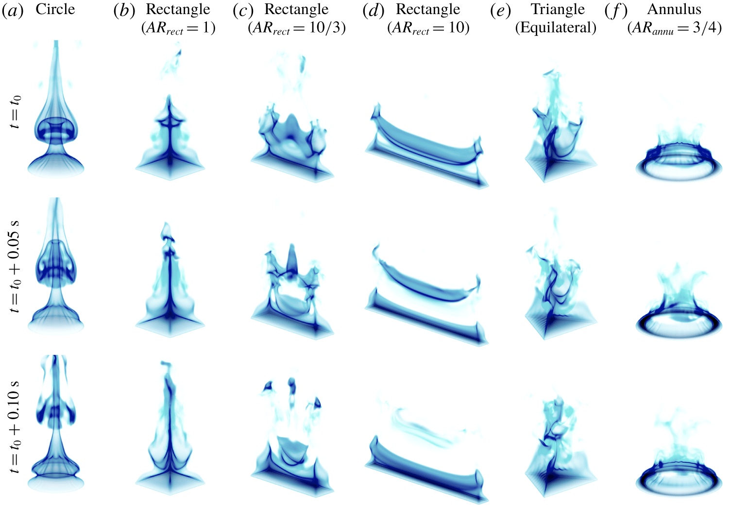
Figure 7 shows time series of temperature isosurfaces for each of the inlet geometries, with  $V_{0}=0.25~\text{m}~\text{s}^{-1}$ in each case. For the circular inlet in figure 7(a), the hot air entering the domain is lighter than the ambient air and is accelerated upwards along the centreline due to buoyancy. The more dense ambient air resting on top of the less dense inlet gases forms a Rayleigh–Taylor (RT) instability which drives the upward motion of the plume. The upward acceleration of the plume subsequently causes entrainment of more dense cold air from the sides, pinching the hot gases towards the centre of the inlet and creating a shear layer between the hot gases and cooler ambient air. This shear layer, combined with the difference in density across the layer, leads to an axisymmetric Kelvin–Helmholtz (KH) instability around the circumference of the inlet. The combination of the RT and KH instabilities causes a roll-up into a toroidal vortex ring that eventually pinches off and is shed, as indicated by the sequence of toroidal temperature isosurfaces rising above the inlet in figure 7(a).
Both the RT instability and shear-driven KH instability impact the overall flow field in these buoyant jets and plumes. Recently, Chakravarthy et al. (Reference Chakravarthy, Lesshafft and Huerre2018) performed a sensitivity analysis of the growth rate of round buoyant jets and plumes over a wide range of Richardson numbers, spanning  $Ri_{D}=10^{-4}$–
 $10^{3}$. They found that, for buoyant jets with low Richardson numbers (i.e.,
 $Ri_{D}=10^{-4}$–
 $10^{0}$), shear and the associated KH instability played a dominant role in the growth of the global flow instability, with baroclinic torque contributing less. However, for buoyant plumes with larger Richardson numbers (i.e.,
 $Ri_{D}=10^{0}$–
 $10^{3}$) buoyancy had a much larger impact, and for Richardson numbers larger than 100, the baroclinic torque was a stabilizing force and did not contribute to the growth of the overall instability.
Isosurfaces of the temperature field as a function of time (snapshots are separated by 0.05 s) for (a) a circular buoyant jet with  $D=0.154$ m; (b–d) rectangular buoyant jets with
 $AR_{rect}=1,10/3,10$; (e) an equilateral triangle buoyant jet with side
 $0.208$ m; (f) an annular buoyant jet with
 $AR_{annu}=3/4$. The inlet velocity in each case was
 $V_{0}=0.25~\text{m}~\text{s}^{-1}$.

Figure 7(b) shows that the flow evolution for an  $AR_{rect}=1$ rectangular inlet is similar to that of the circular inlet, although the resulting structures differ. Hot air is still accelerated upwards upon entering the domain due to the buoyant force, again leading to entrainment of cold air from the sides and pinching of the hot gases towards the centroid of the square. However, the entrained flow along the sides of the inlet reaches the centroid before the flow originating from the corners. This leads to the roll-up and shedding of vortical structures (again indicated by the temperature isosurfaces) that are less coherent than in the circular case shown in figure 7(a).
As the aspect ratio of the rectangle increases to  $AR_{rect}=10/3$ and
 $10$, shown in figures 7(c) and (d), respectively, the shed vortical structures become increasingly elongated. Since the aspect ratio is greater than one in these cases, the long sides of the rectangle are closer to the centroid than the short sides and, as a result, the long-sided shear layer pinches off before the short-sided shear layer has time to develop. This causes the shedding of elongated vortices that are reminiscent of stretched vortex rings.
For the equilateral triangle inlet in figure 7(e), the entrained flow from the sides reaches the centroid before the flow from the corners. This results in the formation of a three-sided vortical structure similar to the four-sided vortical structure of the square buoyant jet in figure 7(b).
Finally, figure 7(f) shows the structure and development of the buoyant jet for the annular inlet. As the hot air enters the domain, ambient air is again entrained, not towards the centreline of the shape, but rather towards the average of the inner and outer radii (i.e., directly above each section of the inlet). This location of converging flow and subsequent puffing causes ambient air to be entrained in the negative radial direction at locations greater than the outer radius, and in the positive radial direction at locations less than the inner radius. Consequently, the shear layer, roll-up and subsequent shedding of vortical structures are all centred above the average of the inner and outer radii. This results in toroidal vortices within the inner radius that create a net downward motion at the centre of the annulus and counteract the upward acceleration of fluid due to buoyancy.
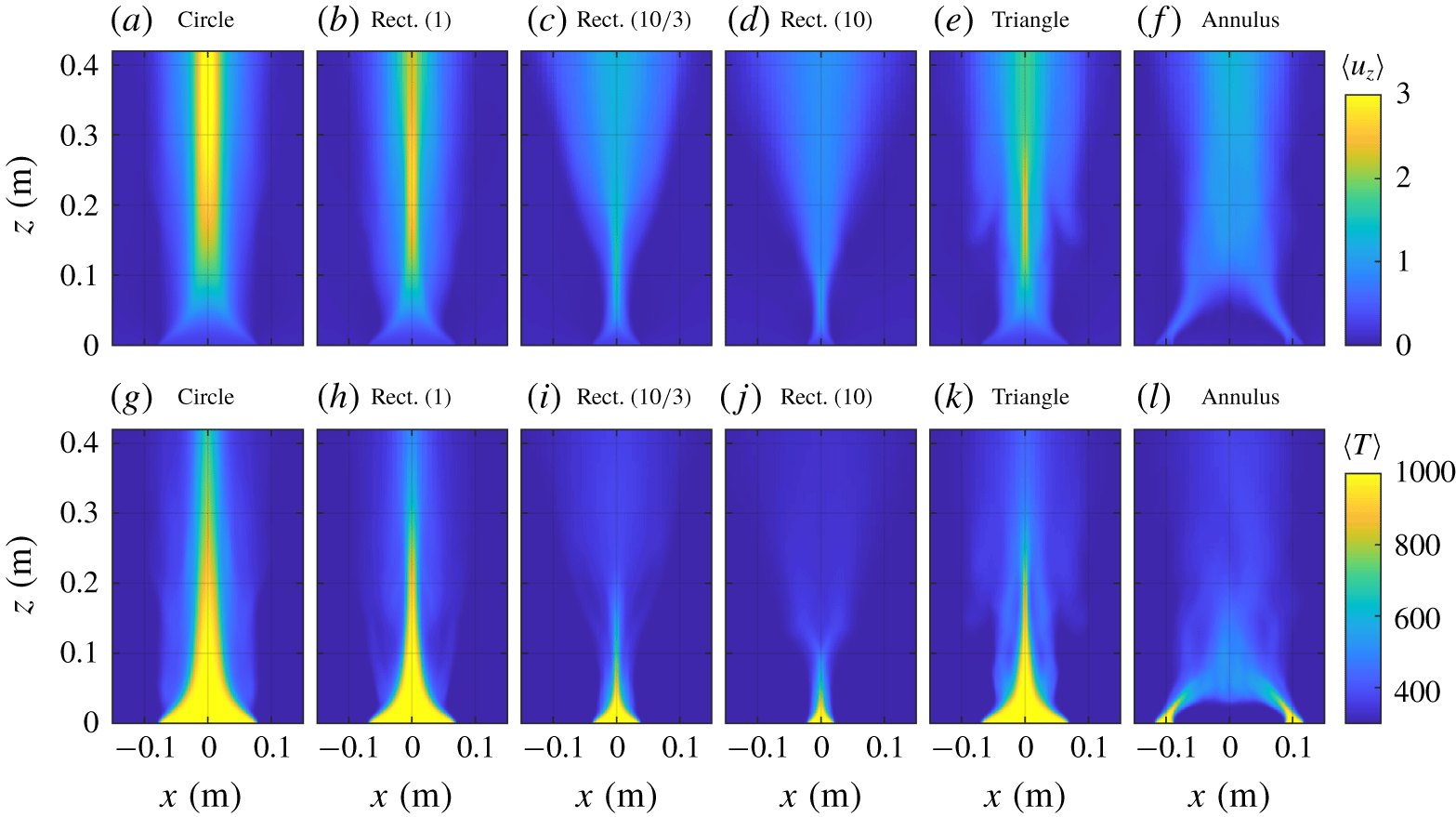
Two-dimensional fields of the time-averaged vertical velocity  $\langle u_{z}\rangle$ in
 $\text{m}~\text{s}^{-1}$ (a–f) and the time-averaged temperature
 $\langle T\rangle$ in K (g–l) for (a,g) a circular buoyant jet with
 $D=0.154$ m; (b–d,h–j) rectangular buoyant jets with
 $AR_{rect}=1,10/3,10$; (e,k) an equilateral triangle buoyant jet with side
 $0.208$ m; (f,l) an annular buoyant jet with
 $AR_{annu}=3/4$. The inlet velocity in each case was
 $V_{0}=0.25~\text{m}~\text{s}^{-1}$ and the planes along which the 2-D fields are shown are indicated in figure 1.

3.2 Flow statistics
Figure 8 shows 2-D fields of the time-averaged vertical velocity,  $\langle u_{z}\rangle$, and time-averaged temperature
 $\langle T\rangle$ for the same six cases shown in figure 7. Each of the cases reveals an increase in the vertical velocity above the inlet due to buoyancy, although the greatest increases are observed for the circle, square (
 $AR_{rect}=1$) and equilateral triangle inlets shown in figure 8(a,b,e). As compared to the other inlet shapes, the high-temperature flow correspondingly extends higher into the domain for each of these cases, as shown in figure 8(g,h,k). For the annulus shown in figure 8(f,l), there is a rapid ‘necking’ inwards of the flow from the inlet, with flow from the two sides of the inlet merging at roughly half a diameter above the centre of the annulus.
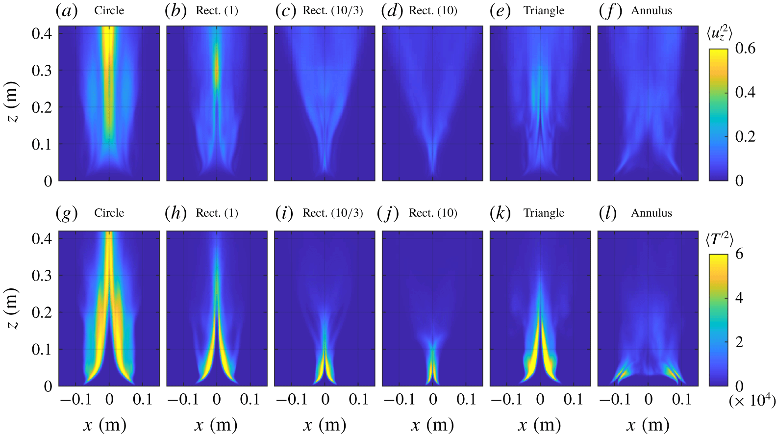
Two-dimensional fields of the time-averaged vertical velocity variance  $\langle u_{z}^{\prime 2}\rangle$ in
 $\text{m}^{2}~\text{s}^{-2}$ (a–f) and the time-averaged temperature variance
 $\langle T^{\prime 2}\rangle$ in
 $\text{K}^{2}$ (g–l) for (a,g) a circular buoyant jet with
 $D=0.154$ m; (b–d,h–j) rectangular buoyant jets with
 $AR_{rect}=1,10/3,10$; (e,k) an equilateral triangle buoyant jet with side 0.208 m; (f,l) an annular buoyant jet with
 $AR_{annu}=3/4$. The inlet velocity in each case was
 $V_{0}=0.25~\text{m}~\text{s}^{-1}$ and the planes along which the 2-D fields are shown are indicated in figure 1.

Variances of vertical velocity and temperature,  $\langle u_{z}^{\prime 2}\rangle$ and
 $\langle T^{\prime 2}\rangle$, respectively, are shown for each of the inlet shapes in figure 9. Once again, fields for the circle, square (
 $AR_{rect}=1$) and equilateral triangle inlets are qualitatively similar, with larger vertical velocity variances along the centreline and higher in the domain, and larger temperature variances along the interface between the low-temperature ambient fluid and high-temperature inlet fluid. Interestingly, there are similarities in the temperature variance fields for the high aspect ratio rectangle (
 $AR_{rect}=10$) and annular inlets shown in figures 9(j) and 9(l), respectively, with flow at the annulus inlet resembling a high aspect ratio rectangular inlet directed at an angle towards the centre of the annulus.
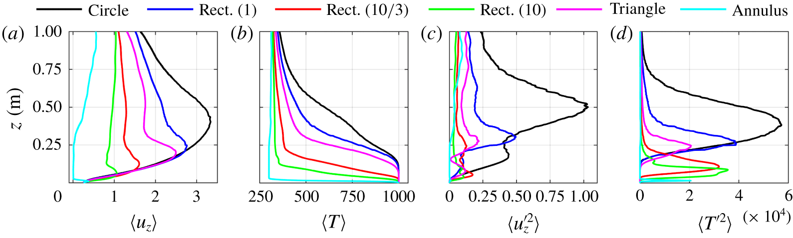
(a) Centreline profiles of the time-averaged vertical velocity  $\langle u_{z}\rangle$ in
 $\text{m}~\text{s}^{-1}$, (b) the time-averaged temperature
 $\langle T\rangle$ in K, (c) the vertical velocity variance
 $\langle u_{z}^{\prime 2}\rangle$ in
 $\text{m}^{2}~\text{s}^{-2}$ and (d) the temperature variance
 $\langle T^{\prime 2}\rangle$ in
 $\text{K}^{2}$ for a circular buoyant jet with
 $D=0.154$ m, rectangular buoyant jets with
 $AR_{rect}=1,10/3,10$, an equilateral triangle buoyant jet with side 0.208 m and an annular buoyant jet with
 $AR_{annu}=3/4$. The inlet velocity in each case was
 $V_{0}=0.25~\text{m}~\text{s}^{-1}$.

Centreline profiles of the first- and second-order statistics of  $u_{z}$ and
 $T$ are shown for each of the inlet shapes in figure 10. Note that the profile for the annulus is taken above the centre of the annulus inlet, as opposed the geometric centre of the annulus as a whole. Figure 10(a,b) shows that there is a general similarity in the profiles of
 $\langle u_{z}\rangle$ and
 $\langle T\rangle$ between the different shapes, with
 $\langle u_{z}\rangle$ increasing immediately above the inlet for all but the annulus, and
 $\langle T\rangle$ decreasing. The rapid decreases in
 $\langle u_{z}\rangle$ and
 $\langle T\rangle$ above the inlet for the annulus are due to the inward angling of the flow from the inlet for this case, as shown in figures 8 and 9. Centreline profiles of the variances
 $\langle u_{z}^{\prime 2}\rangle$ and
 $\langle T^{\prime 2}\rangle$ in figure 10(c,d) again reveal qualitative similarities in the circle, square (
 $AR_{rect}=1$) and equilateral triangle inlets, with the largest variances observed for the circle. Across each of the first- and second-order statistics examined here, there are generally substantial similarities in the fields and profiles for the two higher aspect ratio rectangular cases.
3.3 Puffing frequencies
For each of the inlet shapes examined here, the sequence of vertical buoyancy-driven flow associated with the RT instability, entrainment of ambient air, pinching of hot gases, development of the KH instability, and subsequent shedding of vortical structures outlined in § 3.1 and shown in figure 7 is repeated indefinitely, resulting in characteristic puffing frequencies for each case. From a quantitative perspective, the dominant puffing frequency can be determined using a number of methods, and here we use a fast Fourier transform (known as FFT) of the vertical velocity time series at a point above the centroid of the circular, rectangular and triangular buoyant jets, and above the average radius for the annular buoyant jet. The dominant frequency was found not to depend on height above the inlet within the near field, and a height equal to the hydraulic radius  $R_{h}=A/P$ was thus used for each case, where
 $A$ is the geometric area of the inlet and
 $P$ is its perimeter. Figure 1 provides formulae for
 $A$ and
 $P$ for each of the inlet shapes.
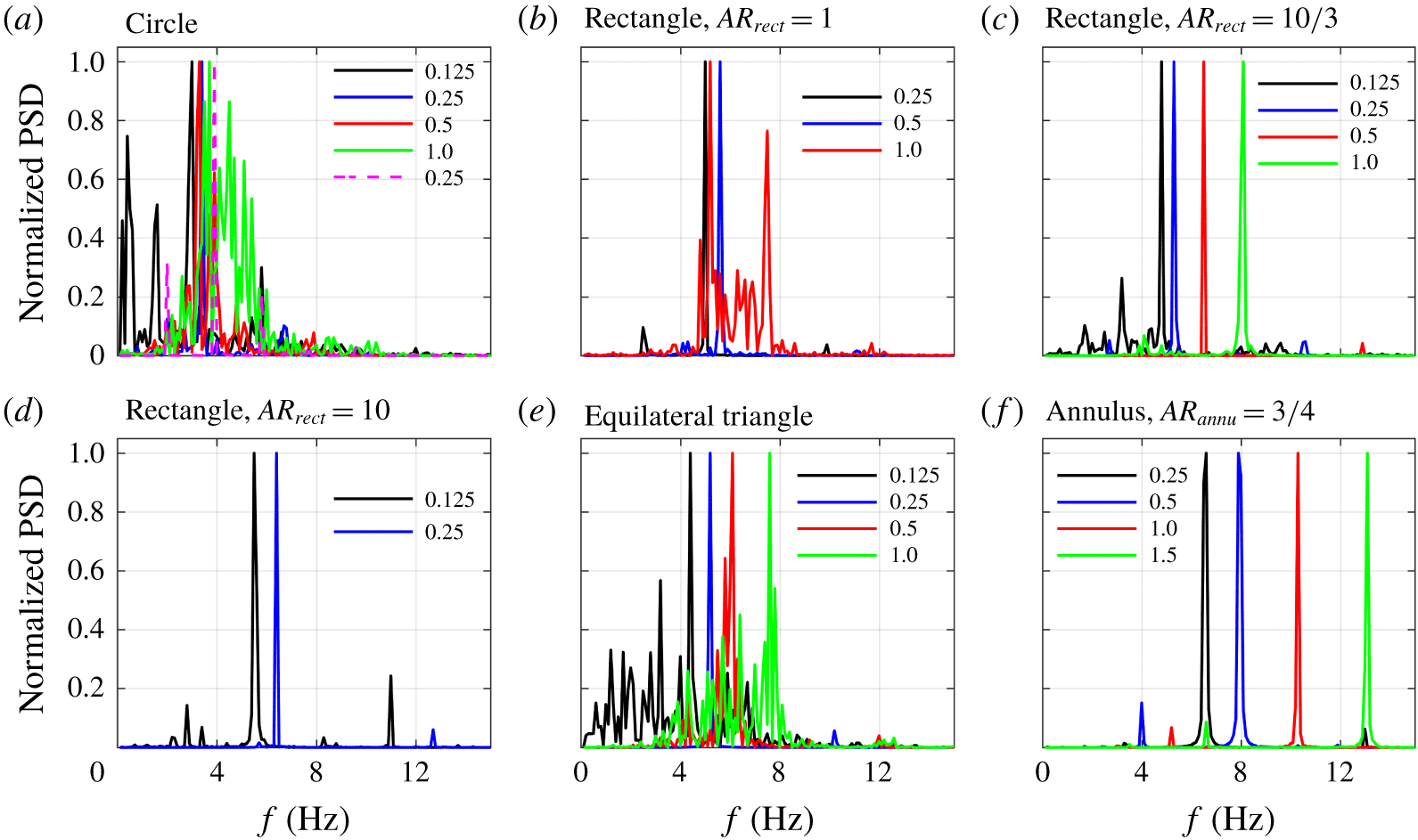
Power spectral densities of the vertical velocity for (a) circular; (b–d) rectangular (with  $AR_{rect}=1,10/3,10$); (e) triangular; (f) annular buoyant jets. Inlet velocities,
 $V_{0}$, are indicated in the legends in units of
 $\text{m}~\text{s}^{-1}$. In panel (a), solid lines denote results for the
 $D=0.274$ m inlet and the dashed line corresponds to the
 $D=0.154$ m inlet. Power spectral densities are computed one hydraulic radius above the inlet centroid for the circular, rectangular, and triangular inlets, and above the average radius for the annular inlet.

The resulting power spectral densities, shown in figure 11, display distinct peaks for each of the inlet shapes and velocities. Peak frequencies increase with inlet velocity for all shapes, and a comparison of the three rectangular cases in figure 11(b–d) shows that the peak frequencies also increase as the aspect ratio increases. The highest peak frequencies are obtained for the annular case shown in figure 11(f). Notably, despite the self-interacting nature of the annular buoyant jet and the subsequent difference in structure compared to the other inlet shapes, the flow still exhibits a characteristic puffing behaviour. This indicates that the puffing phenomenon is largely independent of the inlet shape, and is instead determined by the underlying dynamics associated with buoyancy and the RT instability, entrainment, pinching, KH roll-up and vortex shedding.
4 Discussion
Following the analysis outlined in Bharadwaj & Das (Reference Bharadwaj and Das2017) for helium jets and plumes and in Chakravarthy et al. (Reference Chakravarthy, Lesshafft and Huerre2018) for thermal jets and plumes, five non-dimensional groups can be formed from the dominant puffing frequency  $f$, the parameters that describe the high- temperature flow of air through the inlet (i.e.,
 $V_{0}$,
 $\ell$,
 $\unicode[STIX]{x1D70C}_{0}$,
 $\unicode[STIX]{x1D707}_{0}$,
 $\unicode[STIX]{x1D706}_{0}$; see table 1), and the gravitational acceleration
 $g$; namely
 $$\begin{eqnarray}\displaystyle St_{\ell }=\frac{f\ell }{V_{0}},\quad Re_{\ell }=\frac{\unicode[STIX]{x1D70C}_{0}V_{0}\ell }{\unicode[STIX]{x1D707}_{0}},\quad Fr_{\ell }=\frac{V_{0}}{\sqrt{g\ell }},\quad Pr_{0}=\frac{\unicode[STIX]{x1D707}_{0}}{\unicode[STIX]{x1D70C}_{0}\unicode[STIX]{x1D706}_{0}},\quad S=\frac{\unicode[STIX]{x1D70C}_{0}}{\unicode[STIX]{x1D70C}_{\infty }}, & & \displaystyle\end{eqnarray}$$
where these parameters correspond, respectively, to the Strouhal, Reynolds, Froude and Prandtl numbers, as well as the density ratio,  $S$. Although some prior studies have focused on the separate effects of
 $Fr_{\ell }$ and
 $S$ on
 $St_{\ell }$ (e.g., Soteriou, Dong & Cetegen Reference Soteriou, Dong and Cetegen2002, Nichols, Schmid & Riley Reference Nichols, Schmid and Riley2007, Bharadwaj & Das Reference Bharadwaj and Das2017), it is common to instead combine these two parameters into the Richardson number as
 $Ri_{\ell }=(1-S)Fr_{\ell }^{-2}$ (Bharadwaj & Das Reference Bharadwaj and Das2019), and this is the approach taken in the current study. This is equivalent to replacing
 $g$ with the reduced gravity
 $g^{\prime }=g(1-\unicode[STIX]{x1D70C}_{0}/\unicode[STIX]{x1D70C}_{\infty })$ in the dimensional analysis, reflecting the fact that
 $g$ is only a relevant parameter when density differences are present in the flow. It should be noted that temperature
 $T$ is not included in the dimensional analysis, since, for a constant inflow pressure
 $p_{0}$ and composition (taken to be air at atmospheric pressure),
 $\unicode[STIX]{x1D70C}_{0}$ and
 $T_{0}$ are inversely proportional, yielding
 $T_{0}/T_{\infty }=S^{-1}$. The mass diffusivities
 $D_{\unicode[STIX]{x1D6FC}}$ are also not included since the present simulations consist of hot air flowing into cooler ambient air, and thus the thermal diffusivity
 $\unicode[STIX]{x1D706}_{0}$ and Prandtl number
 $Pr_{0}$ are of greater relevance. Ultimately, the primary focus in many prior studies has been to determine the dependence of
 $St_{\ell }$ on
 $Ri_{\ell }$ and the remaining non-dimensional parameters, and we follow a similar approach here.
To this end, prior work on round and planar buoyant jets has shown that  $St_{\ell }$ is independent of
 $Re_{\ell }$ (Cetegen Reference Cetegen1997), and we consequently do not examine the dependence of
 $St_{\ell }$ on
 $Re_{\ell }$ here. Similarly, although some differences between helium and thermal buoyant plumes have been identified (e.g., through comparison of the global linear stability analyses by Bharadwaj & Das (Reference Bharadwaj and Das2017) and Chakravarthy et al. (Reference Chakravarthy, Lesshafft and Huerre2018)),
 $Pr_{0}$ is typically close to unity (it is 0.71 in the present simulations; see table 1) and is not considered further here. However, both the Prandtl and Schmidt numbers likely do have an effect on
 $St_{\ell }$ for values that differ substantially from unity, and deserve further study in the future. Following previous studies, we thus seek a scaling relation of the form
 $St_{\ell }=bRi_{\ell }^{a}$, where
 $a$ and
 $b$ are constants that will be determined from the present simulations.
It is worth noting that, in order for  $f$ to increase with inlet velocity
 $V_{0}$, as is suggested for all inlet shapes by figure 11, the exponent
 $a$ must be smaller than
 $1/2$. Prior empirical scaling relations have all been consistent with this constraint; for example, for round buoyant jets, Cetegen & Kasper (Reference Cetegen and Kasper1996) found
 $a=0.38$ for
 $1<Ri_{D}<100$ and
 $a=0.28$ for
 $Ri_{D}>100$, and for planar buoyant jets, Cetegen et al. (Reference Cetegen, Dong and Soteriou1998) found
 $a=0.45$ for
 $1<Ri<100$, with no secondary scaling relation reported.
Prior scaling relations between  $St_{\ell }$ and
 $Ri_{\ell }$ have primarily used a characteristic length scale
 $\ell$ associated with the diameter or width of the inlet. As an initial step, here we follow a similar approach and examine the scaling of
 $St_{\ell }$ using width-based length scales for each inlet shape. For the circular inlets,
 $\ell$ is taken to be the diameter,
 $D$. For the three rectangular inlets, the smallest side length (i.e., the width,
 $W$) is used for
 $\ell$, since this is the scale most relevant to the pinching and subsequent shedding of vortical structures. For equilateral triangles, similar to squares, the length of one side is used for
 $\ell$. Finally, for the annulus,
 $\ell$ is taken to be the difference between the outer and inner radii, i.e.,
 $\ell =(D_{out}-D_{in})/2$.
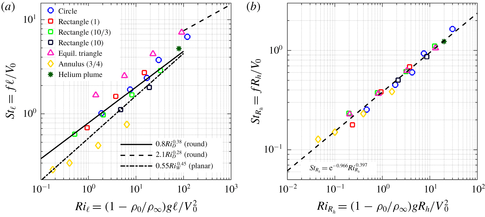
Strouhal number as a function of Richardson number for circular, rectangular ( $AR_{rect}=1,10/3,10$), triangular (equilateral) and annular (
 $AR_{annu}=3/4$) buoyant jets. Panel (a) shows results for characteristic lengths
 $\ell$ based on the diameter (circles), width (rectangles), side (triangles) and the difference between outer and inner radii (annuli). Panel (b) shows results when the characteristic length is taken to be the hydraulic radius,
 $R_{h}$. Scaling relations from Cetegen & Kasper (Reference Cetegen and Kasper1996) and Cetegen et al. (Reference Cetegen, Dong and Soteriou1998) are also shown in panel (a), and a least squares fit to the data is shown in panel (b).

Figure 12(a) shows  $St_{\ell }$ versus
 $Ri_{\ell }$ for each of the simulations performed in the present study, as well as for the round helium plume case from Wimer et al. (Reference Wimer, Day, Lapointe, Makowiecki, Glusman, Daily, Rieker and Hamlington2019). Scaling relations from prior experimental studies of round (Cetegen & Kasper Reference Cetegen and Kasper1996) and planar (Cetegen et al. Reference Cetegen, Dong and Soteriou1998) buoyant jets are also shown. The circular buoyant jet results follow the round jet scaling relations from Cetegen & Kasper (Reference Cetegen and Kasper1996), including an apparent transition at
 $Ri_{D}\approx 100$. The rectangular buoyant jet results fall between prior round and planar scaling relations, with the lower aspect ratio rectangles more closely resembling the round scaling and the higher aspect ratio rectangles more closely resembling the planar scaling. The latter correspondence occurs because, as the rectangle becomes longer relative to its width (i.e., as aspect ratio increases), locations above the centroid appear more and more two-dimensional as corner effects become increasingly negligible. The triangular buoyant jet results follow a similar relation to that for the circular buoyant jets, but with larger values of
 $St_{\ell }$. Interestingly, the annular buoyant jets also closely follow the round jet scaling slope, but with smaller values of
 $St_{\ell }$.
Although scaling relations for each of the different inlet shapes could be obtained separately using least squares fits to the data in figure 12(a), we instead seek a single scaling relation between appropriately defined Strouhal and Richardson numbers for any inlet shape. Similar to the recent work by Bharadwaj & Das (Reference Bharadwaj and Das2019), here we use Strouhal and Richardson numbers, denoted  $St_{R_{h}}$ and
 $Ri_{R_{h}}$, respectively, based on the hydraulic radius of the inlet,
 $R_{h}$, as the characteristic length
 $\ell$ (in their study, Bharadwaj & Das (Reference Bharadwaj and Das2019) used the hydraulic diameter, but this differs from
 $R_{h}$ simply by a constant factor of
 $4$, which we have chosen to exclude in favour of the simpler expression for
 $R_{h}$ in terms of just the inlet area,
 $A$, and perimeter,
 $P$). As an example, the hydraulic radius of a circle with diameter
 $D$ is
 $R_{h}=\unicode[STIX]{x03C0}(D/2)^{2}/(\unicode[STIX]{x03C0}D)=D/4$, and the functional forms of
 $R_{h}$ for other inlet shapes are similarly straightforward to determine from the expressions for
 $A$ and
 $P$ in figure 1.
It should be noted that there is substantial reason to suspect the importance of the hydraulic radius in the formulation of a geometry-independent scaling relation for the puffing Strouhal number. As has already been noted, Bharadwaj & Das (Reference Bharadwaj and Das2019) recently showed that Strouhal and Richardson numbers based on the hydraulic diameter resulted in a single scaling relation for a series of rectangular buoyant jets with different aspect ratios; the present study seeks to determine whether a similar collapse can be achieved when using the hydraulic radius for other shapes. From a physical standpoint, the inlet area and perimeter used to determine the hydraulic radius are also dynamically significant; the area determines, in part, the total buoyancy flux introduced into the domain, and the shear layer that leads to KH roll-up and subsequent vortex shedding forms along the inlet perimeter.
Figure 12(b) shows the resulting relationship between  $St_{R_{h}}$ and
 $Ri_{R_{h}}$ for each of the inlet shapes and velocities. Most notably, all results now fall close to a single scaling relation that was determined using a least squares fit to be
 $St_{R_{h}}=\text{e}^{-0.966}Ri_{R_{h}}^{0.397}$, with an
 $r^{2}=0.981$ coefficient of determination. The secondary scaling associated with circular buoyant jets, observed by Cetegen & Kasper (Reference Cetegen and Kasper1996), is eliminated, and all round buoyant jets, including the helium plume simulation from Wimer et al. (Reference Wimer, Day, Lapointe, Makowiecki, Glusman, Daily, Rieker and Hamlington2019), follow the same scaling relation. Additionally, the various rectangular, triangular and annular results all also follow this relation.
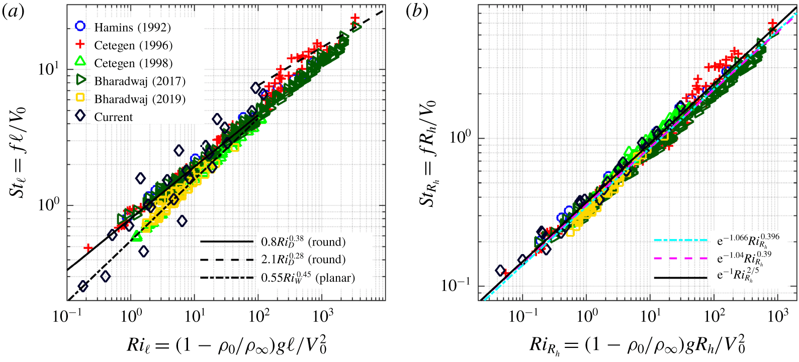
Given the collapse demonstrated in figure 12(b), an obvious next question is whether a similar collapse can be achieved using the broad range of prior experimental studies described in § 1. Figure 13 shows data from the present simulations along with all prior experimental data from Hamins et al. (Reference Hamins, Yang and Kashiwagi1992), Cetegen & Kasper (Reference Cetegen and Kasper1996) and Cetegen et al. (Reference Cetegen, Dong and Soteriou1998), as well as recent experimental data from Bharadwaj & Das (Reference Bharadwaj and Das2017, Reference Bharadwaj and Das2019). Figure 13(a) shows that, once again, when we use a width- or diameter-based formulation for  $\ell$, there is no single scaling relation that accurately describes all available data.
Strouhal number as a function of Richardson number for the present simulations and prior experiments from Hamins et al. (Reference Hamins, Yang and Kashiwagi1992), Cetegen & Kasper (Reference Cetegen and Kasper1996), Cetegen et al. (Reference Cetegen, Dong and Soteriou1998), Bharadwaj & Das (Reference Bharadwaj and Das2017) and Bharadwaj & Das (Reference Bharadwaj and Das2019) (see legend in (a)). Definitions of  $\ell$ in (a) and (b) are the same as those in figure 12. In (b), we also show the least squares fit to all data (cyan dash-dot line), the linear stability analysis result from Bharadwaj & Das (Reference Bharadwaj and Das2017) (magenta dashed line), as well as the proposed relationship from (4.2) (solid black line).

However, when the Strouhal and Richardson numbers are instead computed using the hydraulic radius, the experimental and computational results all fall close to a single line, as shown in figure 13(b). The least squares fit to all available data is  $St_{R_{h}}=\text{e}^{-1.066}Ri_{R_{h}}^{0.396}$ with
 $r^{2}=0.984$, which is close to the scaling relation obtained for the simulation data alone (see figure 12b). Figure 13(b) also shows that the data are accurately described by the scaling relation
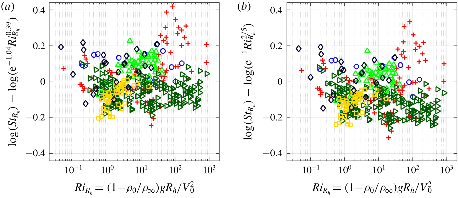
 $St_{R_{h}}=\text{e}^{-1.04}Ri_{R_{h}}^{0.39}$ obtained by Bharadwaj & Das (Reference Bharadwaj and Das2017) from global linear stability analysis of round buoyant jets and plumes. This agreement is also demonstrated by the residuals between the available computational and experimental data and the scaling relation from linear stability analysis shown in figure 14(a).
Based on the current simulation and prior experimental results shown in figure 13(b), as well as the similarity of the computed scaling coefficients to rational numbers, we propose the following shape-independent scaling relation between  $St_{R_{h}}$ and
 $Ri_{R_{h}}$:
 $$\begin{eqnarray}St_{R_{h}}=\text{e}^{-1}Ri_{R_{h}}^{2/5}.\end{eqnarray}$$
The coefficient of determination between this relation and the simulation and experimental data is  $r^{2}=0.976$. The accuracy of the proposed relation compared to the data can also be determined by examining the residuals of the data with respect to the proposed fit, as shown in figure 14(b). For the proposed relation to be considered an acceptable fit to the data, the residuals should be scattered about zero and show no discernible trends with respect to the dependent variable (i.e.,
 $Ri_{R_{h}}$). Figure 14(c) shows that the residuals for all current and prior data are scattered about zero, indicating the lack of any persistent bias in (4.2) with respect to this data. It is worth noting that Bharadwaj & Das (Reference Bharadwaj and Das2019) used an effective velocity instead of
 $V_{0}$ in their scaling relations, but the data collapse shown in figures 12 and 13 was found not to require this correction.
(a) Residuals between the linear stability relation from Bharadwaj & Das (Reference Bharadwaj and Das2017) and (b) the proposed scaling relation from (4.2) for the present simulations and prior experiments from Hamins et al. (Reference Hamins, Yang and Kashiwagi1992), Cetegen & Kasper (Reference Cetegen and Kasper1996), Cetegen et al. (Reference Cetegen, Dong and Soteriou1998), Bharadwaj & Das (Reference Bharadwaj and Das2017) and Bharadwaj & Das (Reference Bharadwaj and Das2019) (see legend in figure 13a).

It is emphasized that (4.2) is an empirical proposed relation that is suggested by results from simulations, experiments and stability analyses. Further research is required to determine whether this relation can be given a theoretical basis, as well as the range of Richardson numbers and inlet geometries over which it is valid. Nevertheless, support for this relation is provided by a broad range of sources. In particular, nearly all prior scaling relations have yielded scaling exponents of 0.4, when rounded to one decimal, and it is difficult given experimental uncertainties (many of which were discussed in Bharadwaj & Das (Reference Bharadwaj and Das2017)) to determine whether differences in the next decimal place are statistically significant, particularly when comparing results collected over nearly thirty years from widely different experimental and simulation configurations for both helium and thermal buoyant flows.
5 Conclusions
Adaptive mesh numerical simulations of buoyant jets and plumes have been performed for seven different inlet shapes: two circular inlets (corresponding to different diameters), three rectangular inlets (corresponding to different aspect ratios), an equilateral triangle inlet and an annular inlet. A range of inlet velocities were simulated for each geometry, giving a range of inlet Richardson numbers for each case, and the resulting puffing Strouhal numbers were measured above the inlets.
Fundamental aspects of the flow evolution were found to be similar for each of the inlet shapes, including the buoyant rise of hot inlet gases and the associated RT instability, entrainment of cold ambient gases, pinching of the hot gases towards a central location above each inlet, formation of a KH instability along the interface between the hot and cold gases, and the subsequent pinch-off and shedding of vortical structures. This process was observed for each inlet shape, but the shed vortices were found to become less coherent as the complexity of the inlet increased. We found that, in general, the puffing frequency increased with inlet velocity and, for the rectangular cases, aspect ratio.
Using width-based puffing Strouhal and inlet Richardson numbers, our results are consistent with prior experimental studies of round and planar jets, with the highest aspect ratio rectangular cases examined here closely corresponding to prior planar results. However, when using such width-based non-dimensional parameters, we did not find a single scaling relation that accurately describes the Strouhal–Richardson relationship for all inlet shapes.
By contrast, if we instead use Strouhal and Richardson numbers based on the hydraulic radius, similar to the use of hydraulic diameter coupled with an effective velocity by Bharadwaj & Das (Reference Bharadwaj and Das2019), we do recover a single scaling relation, given in (4.2), that accurately describes the present computational results and prior planar and round experimental data. The scaling relation in (4.2) was found to closely describe both experimental and simulation results for Richardson numbers spanning four orders of magnitude. We found that the use of the effective velocity proposed by Bharadwaj & Das (Reference Bharadwaj and Das2019), as opposed to simply the inlet velocity, was not required to obtain consistent agreement between the proposed scaling relation and all other data. Further examination of the potential role of modified forms of the inlet velocity are nevertheless an important direction for future research.
It is tempting to propose (4.2) as a universal scaling relation for buoyant jet puffing that can be applied to any inlet shape. However, a broader range of inlet shapes, spanning a wider range of Richardson numbers, must be examined before this claim can be made with confidence. In particular, complex inlet shapes without any symmetries, or those with narrow connection points, require further study. Given the identification of multiple puffing modes by Bharadwaj & Das (Reference Bharadwaj and Das2017), as well as the transition between the modes at high Richardson number, it is of interest to explore the range of validity of the relation in (4.2), particularly for very low and high Richardson numbers. The rational exponents in (4.2) are also suggestive of a theoretically based scaling relation, and further study may provide a rigorous justification for the proposed exponents. Finally, the present results and scaling relations span both helium and high-temperature buoyant flows, but it is still possible that the Schmidt and Prandtl numbers may have an additional impact on the puffing frequency, and the study of these effects is a further important direction for future research.
Acknowledgements
Helpful discussions with M. S. Day, A. Nonaka and W. J. A. Dahm are gratefully acknowledged and experimental data from Bharadwaj & Das (Reference Bharadwaj and Das2017, Reference Bharadwaj and Das2019) was helpfully provided by D. Das and K. Bharadwaj. N.T.W., G.B.R. and P.E.H. were supported, in part, by the Strategic Environmental Research and Development Program under grant W912HQ-16-C-0026. C.L. was supported by the National Science Foundation Graduate Fellowship Program under grant no. NSF GRFP, DGE 1144083. Gift support from the 3M Company is also gratefully acknowledged.
Declaration of interests
The authors report no conflict of interest.