

More than forty years ago the Supreme Court took a profound step toward improving the equality of political representation in the United States. In a series of cases beginning in 1962, the Court established the “one-person, one-vote” rule.1
See Baker v. Carr, 369 U.S. 186 (1962); Gray v. Sanders, 372 U.S. 368 (1963); Wesberry v. Sanders, 376 U.S. 1 (1964); Reynolds v. Sims, 377 U.S. 533 (1964).
Wesberry, 376 U.S. at 8.
The Supreme Court spoke forcefully against malapportionment by stressing that it was “counter to our fundamental ideas of democratic government,” and if permitted, “it would cast aside the principle of a House of Representatives elected ‘by the People,’ a principle tenaciously fought for and established at the constitutional Convention.”3
Ibid. at 8.
Ibid.
White v. Weiser 412 U.S. 783, 790 (1973). The original wording is drawn from Kirkpatrick v. Preisler, 394 U.S. 526, 531 (1969). In the latter case, the Court found that the population discrepancy of 25,802 individuals between Missouri's largest and a smallest congressional district was unconstitutional.
White, 412 U.S. at 790.
Karcher v. Daggett, 462 U.S. 725 (1983).
Over the past forty years, the Supreme Court vigorously has corrected the intrastate malapportionment of U.S. House districts.8
See Rogowski 1981 for a theoretical discussion of representation and the case history of intrastate malapportionment.
Interstate malapportionment is an unintended and understudied byproduct of four interrelated factors: (1) uneven population distribution among the states; (2) territorially defined congressional districts; (3) current apportionment method; and (4) the fixed and limited size of 435 members in the House of Representatives. Intentionally or not, the House has become systematically malapportioned and is likely to become only more so over time. The constitutional, normative, and practical implications of either form of malapportionment are similar. Intrastate malapportionment and interstate malapportionment, though, are quantitatively different; the latter is currently significantly more severe. Based on the 2000 reapportionment, the interstate population discrepancy between two House districts is as much as 410,012 individuals, which is over twenty-one times greater than the intrastate malapportionment ruled unconstitutional in White. Despite the Court's aggressive stance toward intrastate malapportionment, it declined its only opportunity to date to address interstate malapportionment.9
U.S. Commerce v. Montana, 503 U.S. 442 (1992).
White, 412 U.S. at 790, emphasis added.
We argue that interstate malapportionment is all too often overlooked by democratic theorists, political analysts, and the public even though it unnecessarily undermines the procedural recognition of the electoral political equality and fairness embodied by the U.S. House. It also inhibits a fuller establishment of the one-person, one-vote principle. We intentionally say “fuller” instead of “full” because an analysis of the causes of interstate malapportionment also points toward a fundamental paradox between the Constitution's mandate, accepted standards of representative legitimacy, and the Court's current requirements for congressional constituencies. Nonetheless, we suggest that changing the fourth factor, namely, the fixed size of House membership, is the most reasonable and measured solution, albeit limited, to the problem of interstate malapportionment.
The Causes of Interstate Malapportionment
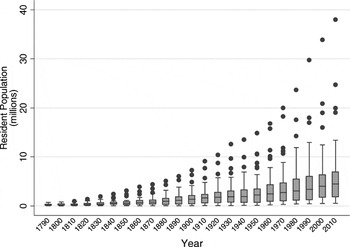
The first cause of interstate malapportionment is uneven population distribution among the states. We assume this requires little verification. Since the founding of the country, its population has grown and so have the average and median state populations. The populations of small and large states, however, have not grown at the same rate, and accordingly, the standard deviation of the mean has increased each year. Figure 1 plots some of the summary statistics for state populations from 1790 to 2010.11
The state population figures for 2010 are, of course, estimates. They are calculated by extrapolating from the population growth rates between 1990 and 2000 for each state. Only resident populations were readily available for the entire time series. Resident and apportionment populations differ in that the latter also includes overseas residents. The difference is relatively insignificant. In 2000, there was a total of 574,330 residents officially registered overseas; the state with the largest number (California) had 59,150 overseas residents (0.175 percent); the state with the largest percentage (Hawaii) had 5,105 overseas residents (0.421 percent).

State population: Increasingly dispersed and skewed
By itself, however, the uneven distribution of state populations does not cause interstate malapportionment. The second factor, territorially bounded congressional districts, is a necessary condition. The territorially bounded districts in the U.S. Senate, for instance, are obvious. Each state, regardless of population, is represented by two senators. Senate apportionment is specifically designed to represent states equally, not individuals. To balance the Senate's definition of constituency, the Framers, in the Great Compromise, created the House with the intent that it represents individuals.12
Madison, Federalist No. 58, in Kesler and Rossiter, eds., 1999, 325.
Without these territorial constraints on the distribution and construction of House seats, every House district, less one, easily could have exactly as many constituents as the national average. The one remaining district would be at most within ± 218 individuals of the national district average. Given these territorial constraints, however, the only circumstance in which one-person, one-vote could be achieved and interstate malapportionment avoided would be if each and every state always had a population equal to a whole-number multiple of the national district average. This has never—not even remotely—occurred, and there is no reason to assume that it ever would. Hence, as long as House constituencies are geographically defined, House seats will never achieve political equality and will always be malapportioned among states. The Supreme Court has acknowledged as much:
The constitutional guarantee of a minimum of one Representative for each State inexorably compels a significant departure from the ideal. In Alaska, Vermont, and Wyoming, where the statewide districts are less populous than the ideal district, every vote is more valuable than the national average. Moreover, the need to allocate a fixed number of indivisible Representatives among 50 States of varying populations makes it virtually impossible to have the same size district in any pair of States, let alone in all 50. Accordingly, although “common sense” supports a test requiring “a good faith effort to achieve precise mathematical equality” within each State, Kirkpatrick v. Preisler, 394 U.S., at 530-531, the constraints imposed by Article I, 2, itself make that goal illusory for the Nation as a whole.13
U.S. Commerce v. Montana, 503 U.S. at 464.
The third cause of interstate malapportionment is the current apportionment method. Given the presence of territorial House boundaries and the absence of state populations equal to a whole-number multiple of the national district average, true political equality calls for some fraction of a representative. As the Supreme Court aptly notes, representatives are indivisible: a state that deserves 1.5 representatives only can receive one or two representatives, not 1.5 representatives.14
Ibid.
Balinski and Young 1982, 1.
This may explain, in part, why since the country's founding, Congress has employed or proposed at least six main apportionment methods, plus variants. Each is known by its author's or proponent's name. They include the Adams, Hamilton, Jefferson, Webster, Dean, and Hill methods.16
For a discussion of the methods, the historical use, and the value of each, see Balinski and Young 1982; Darcy 2004; Huckabee 2000, 2001; U.S. Commerce v. Montana, 503 U.S. 442 (1992).
Act of November 15, 1941, 1, 55 Stat. 761–762, 2 U.S.C. 2a.
The fourth cause of interstate malapportionment is that the size of the U.S. House has been fixed at 435 members since 1910.18
The House was briefly increased to 437 members in 1959 to accommodate the statehood of Alaska and Hawaii. It returned to 435 members after the 1960 reapportionment.
Just as important, because House seats are constitutionally apportioned among territorial units (states), and not across the national constituency (individuals), small states are not able to distribute their district population remainders among multiple districts. A state's population remainder is produced by dividing the state's population by the number of its House seats. It is the number of statewide individuals who will be either over- or underrepresented based on the national average of individuals per district. Large states are able to distribute their population remainders among many districts and, thus, each district is more likely to approximate the national average district size. Even if every state constructed its House districts with a perfectly equal numbers of individuals, as required by the Supreme Court's intrastate malapportionment decisions and its one-person, one-vote rule, interstate malapportionment is unavoidable, and it is exacerbated by the fixed and limited size of the House.
The effects of the four causes of interstate malapportionment just discussed, although easily overlooked, have been predictable.19
See Celler 1951.
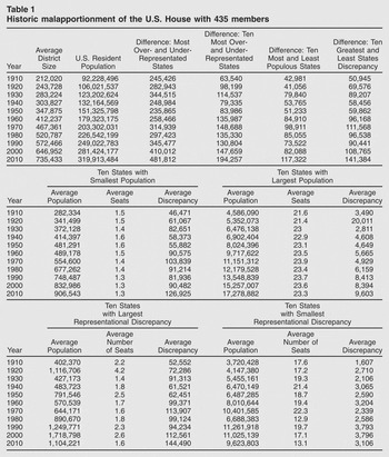
Historic malapportionment of the U.S. House with 435 members

According to figures from the 2000 Census, California's apportionment population was 33,930,798 individuals. The reapportionment based on these data assigned California 53 congressional seats. If one multiplies the national average district size by California's 53 districts and subtracts its actual apportionment population, the equation produces a population remainder of 357,658 (overrepresented) individuals. California, though, was able, and in fact was required, to distribute the remainder among its 53 districts as equally as possible. Thus, California's average district size, 640,204, was nearly the national average. The average discrepancy between California's and the nation's average district size was 6,748 individuals. Even so, California was not the best-apportioned state in 2000. Because of the combination of many districts among which Pennsylvania could distribute its population remainder and a population very near a whole-number multiple of the national district average population, the typical Pennsylvania district had an average discrepancy from the national average of only 452 individuals. Conversely, Utah's population of 2,236,714 individuals entitled it to three House seats, resulting in an average district of 745,571 (underrepresented) individuals. This is an average discrepancy between the state and national average district size of 98,619 individuals: more than 14 times that of California and more than 218 times that of Pennsylvania. The population remainder proves more troublesome for states with only one district. For instance, Montana was malapportioned from the national average by 258,364 (underrepresented) individuals—an average discrepancy more than 38 times that of California and more than 571 times that of Pennsylvania.
Interstate malapportionment is not confined to just a few states. After the 2000 reapportionment, the average discrepancy between the average district size of the ten states with the largest populations and the national average district size was 8,424 individuals; for the ten states with the smallest populations, 90,888 individuals. The calculation of the apportionment discrepancy based solely on population, however, underestimates the extent of the interstate malapportionment. For example, North Dakota had only one district but, like Pennsylvania, had an apportionment population very near a whole-number multiple of the national district average population. As such, North Dakota, with 643,756 individuals, was malapportioned from the national average by only 3,196 individuals. The average discrepancy of the ten states with the smallest apportionment discrepancy was 3,796 individuals; of the ten states with greatest apportionment discrepancy, 112,561 individuals: a difference of nearly 30 times.
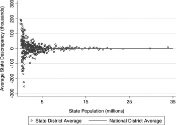
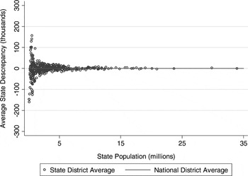
The problem of remainder distribution is a mathematical identity that systematically causes disproportionate interstate malapportionment. Figure 2 displays average state discrepancy and state population from 1920 through 2000—the period during which he House membership was fixed at 435. The average state discrepancy is the number of individuals that each state's average district is either overrepresented (negative numbers) or underrepresented (positive numbers) relative to the national average district size (the flat line at 0) for each decennial apportionment. The pattern is clear: the smaller the state, the greater the likelihood and the greater the extent to which that state is malapportioned. The fixed size of House membership, which limits the ability of a small state to distribute its population remainder adequately, accentuates the problem. If the House were to increase its membership, small states would be apportioned a relatively small number of additional districts and large states would be apportioned a relatively larger number of additional districts. Together, the distribution problem of population remainders would be less acute, which, in turn, would also better approximate equal representation between the small and large states.

Interstate malapportionment by state size: 1920–2000 with 435 members
Although no system of representative democracy will ever be able to meet the one-person, one-vote rule perfectly, a nation with a heterogeneously distributed population, a federal system of representation with territorial constraints, and a legislature without size adjustments causes unusually severe interstate malapportionment—more severe than the malapportionment found in many intrastate cases. Again, after the 2000 reapportionment, one example of interstate malapportionment was more than 21 times greater than the intrastate malapportionment ruled unconstitutional in White.
Although the increase in interstate malapportionment since 1910 is not strictly linear (see table 1), the trend is positive and steep. There are few reasons to anticipate any significant changes in the trend, given the distribution and growth rates of state populations and the attendant constitutional and mathematical issues. Indeed, if each state's population increases at the same rate as it did from 1990 to 2000, the 2010 reapportionment will result in a national average district size of 735,433 and a maximum difference of 481,812 individuals between the most under- and overrepresented districts.20
Population growth rates are calculated using the 1990 and 2000 U.S. Census, and apportionment was assigned using the Equal Portions (Hill) Method as described by the U.S. Census.
Assessing the Remedies for Interstate Malapportionment
Given the nature of the first cause of interstate malapportionment, namely, uneven population distribution among the states, there is little, if anything at all, that can be done about it. The uneven and skewed distribution of state populations is a function of interstate mobility and birth rates. These cannot, or at the very least ought not, be regulated. Reminiscent of Madison's argument in Federalist No.10 about the solutions for the causes of factions: the remedy for the dispersed and skewed state populations is “worse than the disease” because it would require “destroying the liberty which is essential to its existence.”21
Madison, Federalist No. 10, in Kesler and Rossiter, eds., 1999, 72–73.
Assessing the remaining causes is more difficult. To do so, we first need to evaluate the standards by which we judge the adequacy of representative institutions in providing political equality and fairness. In other words, we ask whether interstate malapportionment is something that is normatively unacceptable. Normative acceptability can be assessed, Beitz argues, through a system of complex proceduralism. “Complex proceduralism does not embrace any single value (such as the conservation of power) as definitive of political fairness; it recognizes a plurality of reasons why a procedural regime might be judged to be unfair.”22
Beitz 1989, 100.
Ibid.
Ibid., 107.
Ibid., 106.
Nonetheless, within the context of each issue and institution, there are constraints. Parties are prevented from “seeking procedural advantages for themselves that conflict with [the regulative] interests which all are assumed to share.”26
Ibid., 105.
Ibid., 109. “Reasonableness” is our label of Beitz's concept.
To make specific assessments of the representative institutions of the United States, we begin with the theoretical conceptualizations and practical implications of congressional constituencies. We begin again in the Senate, which naturally begs the question why should we be concerned about interstate malapportionment in the House when the interstate malapportionment in the Senate is so much more severe? The assignment of two senators to every state regardless of population makes the Senate one of most malapportioned chambers in the world.28
Samuels and Snyder 2001.
The Senate's apportionment, however, is explicitly rooted in the Constitution and is specifically designed to represent states, not individuals, equally.29
Dahl 2002 argues that the apportionment of the Senate is a fundamental flaw of the Constitution.
Zagarri 1987.
Since their country's founding, Americans generally have accepted the Senate's apportionment as a unique part of American democracy despite its obvious “undemocraticness.” The Senate, then, seems to exemplify Beitz's argument that political equality and fairness must treat each institution in question as “a freestanding moral issue” and account for “the historical circumstances” that gave rise to the institution. In other words, if Americans generally recognize and accept the inequality inherent in the Senate, then the institution may not violate the normative requirements of political fairness.32
Beitz 1989, 94.
In many ways, evaluating the House is more difficult. The Framers agreed in the Great Compromise to split the difference among them by creating the Senate (to represent place) and the House (to represent individuals). After that, “population equality became the central rule of representation” for the lower chamber.33
Rehfeld 2001, 76. The principle of population equality, though, was certainly not broadly defined. See, for instance, the Three-Fifths Clause of the Constitution.
As the foregoing discussion of the Senate and the House demonstrates, there are different yet legitimate definitions of constituencies and standards of democracy for representative institutions.34
Rehfeld argues that American electoral constituencies “could be (and could have been) defined by descriptive or ascriptive characteristics: for example, by profession, religion, ideology, or identity. They could be defined by race or political party, as territorial districts most often are defined today.”35Rehfeld 2001, 54.
The infinite number and types of extraconstitutional options and their consequences make analyses infeasible for the discreet scope of this study. Thus, in our context, we view amending the Constitution, for instance, to eliminate the territorial boundaries of House districts as “unreasonable.” Our significantly more modest and pragmatic goal is to assess the constitutional procedures and their interpretations as they now stand. This approach also is normatively appealing because it respects Beitz's theory of accepting the unique “historical circumstances” that have surrounded institutional design and development. In accepting the uneven distribution of state populations and the constitutional requirements of territorially defined House districts, we also have accepted the inevitability of interstate malapportionment. But, to invoke the language of the intrastate malapportionment cases, we ask whether the current institutional arrangements make individuals “as mathematically equal as reasonably possible.” This consideration also limits us to statutory changes, and it brings us to the final two causes of interstate malapportionment and their practical consequences.
Because none of the different apportionment methods can eliminate interstate malapportionment entirely, the issue is which method objectively embodies current American standards of democracy with the least bias. This may seem like a straightforward empirical question, but it is not. Leading up to the 1930 Census and reapportionment, debate raged among politicians and mathematicians about the value and bias of each method.37
Balinski and Young 1982, 46–59.
Ibid., 70. The Alabama paradox arises when an apportionment formula assigns a state fewer representatives when the size of the chamber increases. The population paradox arises when a state with a faster growth rate loses a seat to a state with a slower growth rate. The new-state paradox occurs when a new state is provided its “fair” representation and the chamber's size is accordingly increased, but the apportionment for other states is nonetheless affected.
Despite a 1929 National Academy of Sciences report commissioned by House speaker Nicholas Longworth endorsing the Hill method, the issue remained unresolved for the 1930 reapportionment. Because of a coincidental distribution of state populations in 1930, the Hill and Webster methods produced the same apportionment and, thus, Congress balked. According to the 1940 Census, however, the state populations were not similarly aligned. The Hill method, as opposed to the Webster method, would provide one more seat to Arkansas and one less to Michigan. The majority party of Congress, the Democrats, with their base of support in the solidly Democratic South, passed and the president, Democrat Franklin D. Roosevelt, signed legislation designating use of the Hill method. It has been used since, but that has not ended the debate. Reexaminations have questioned Huntington's work.39
Balinski and Young 1982 (51) state that Huntington omitted tables from his work that would have supported the Webster method.
Ibid., 76. Also see Young 2001.
Darcy 2004. Balinski and Young 1982 (53) concur that the Dean method minimizes the absolute difference in constituency size but argue that it does not minimize each state's distance from the quota, or its fair representation.
After the 1990 Census, the Supreme Court had the opportunity to judge the constitutionality and fairness of the different apportionment methods. In U.S. Commerce v. Montana (1992), Montana asserted that the Hill method was unconstitutional and that the Dean method was closer to democratic standards. If the Dean method were to be used instead of the Hill method, Montana, not Washington, would have received the last apportioned House seat (number 435).42
This is the only seat that would have changed after the 1990 Census if the Dean method had been adopted.
The Court concluded that it did not possess the capacity to validate one mathematical method over another, and left resolution of this important constitutional question up to Congress and the public. Writing for the majority, Justice Stevens explained:
What is the better measure of inequality—absolute difference in district size, absolute difference in share of a Representative, or relative difference in district size or share? Neither mathematical analysis nor constitutional interpretation provides a conclusive answer. In none of these alternative measures of inequality do we find a substantive principle of commanding constitutional significance. The polestar of equal representation does not provide sufficient guidance to allow us to discern a single constitutionally permissible course.43
U.S. Commerce v. Montana, 503 at 464. It may be significant to note that Justice Stevens writes about measuring “inequality” instead of invoking the intrastate standard of political equality.
After nearly eighty years of silence since the enactment of the 1929 act, it is important that there be an open and public discussion to assess the apportionment methods and which method best approximates the democratic standards of representation commonly accepted for the House. In addition, there are certainly some noteworthy consequences for the states that would gain or lose seats. Had Montana prevailed in U.S. Commerce v. Montana, it would have doubled its representation in the House. Overall, however, changing apportionment methods would do little to diminish interstate malapportionment. If we compare a switch in methods among the three most-promoted (the Dean, the Hill, and the Webster), only a few of the states and districts would be affected. For the ten apportionments from 1910 to 2000 (the period of the 435-member House), 4,350 seats were apportioned. The cumulative number of seats that would change (i.e., counting, as in U.S. Commerce v. Montana, the switch of one seat from Washington to Montana as a change of two seats), comparing the Dean method to the Hill method, is 14 (0.32 percent), comparing the Hill method to the Webster method, is 20 (0.46 percent), and, comparing the Dean method to the Webster method, is 32 (0.74 percent).44
Because each state is constitutionally guaranteed at least one seat, it could be argued that counting all 435 seats overestimates the number of seats eligible to change and thus underestimates the effects of changing apportionment methods. If we assume, then, that only 385 seats are actually eligible to change, then the percentages of seats that change are 0.36 percent, 0.52 percent, and 0.83 percent, respectively.
The fourth cause of interstate malapportionment is the fixed and limited size of House membership. The apportionment of representatives and the size of their chamber were hotly debated by the Framers. James Madison, in Federalist Nos. 55, 56, and 58, argues in favor of a system of decennial augmentations to the number of House seats and their allotment among the states in accordance with changes in the national and state populations. He asserts repeatedly that the Constitution would ensure such changes. “The foresight of the [constitutional] convention has accordingly taken care that the progress of population may be accompanied with a proper increase of the representative branch of government.”45
Madison, Federalist No. 56, in Kesler and Rossiter, eds., 1999, 317.
Madison, Federalist No. 58, in Kesler and Rossiter, eds., 1999, 324.
Madison's insistence on periodic apportionment augmentations rests on at least two premises. The first is the normative standard of equal representation of individuals that the Framers agreed to in the Great Compromise. Periodic enumerations and reapportionments would ensure that the standard is met, given the constantly changing populations of the states. The delegates to the 1787 Convention were keenly aware that the failure to do so would jeopardize House members' communication and contacts with their local constituencies—a point to which we shall return. The second premise is that the state-based definition of constituency and apportionment of the Senate makes accurate individual-based apportionment of the House imperative. It follows that decennial adjustments to the size of the House membership are of paramount concern for the constitutional balance of power and the proper functioning of American democracy.47
Ibid., 325.
This concern was so paramount to the first Congress that it passed a constitutional amendment to guarantee apportionment augmentations. The amendment was included in the original twelve amendments sent to the states for ratification. The ten that were ratified were to become known, of course, as the Bill of Rights. The first of the original twelve amendments passed by Congress on September 25, 1789, stated the following:
Article the first… After the first enumeration required by the first Article of the Constitution, there shall be one Representative for every thirty thousand, until the number shall amount to one hundred, after which, the proportion shall be so regulated by Congress, that there shall be not less than one hundred Representatives, nor less than one Representative for every forty thousand persons, until the number of Representatives shall amount to two hundred, after which the proportion shall be so regulated by Congress, that there shall not be less than two hundred Representatives, nor more than one Representative for every fifty thousand persons.48
Mount 2004.
The amendment was ratified by one state less than required to add it to the Constitution. In a strange twist of history, the other amendment that failed, which concerned congressional pay raises and was originally passed by six states and rejected by five, became the 27th Amendment to the Constitution in 1992.49
Gregory Watson, a University of Texas undergraduate, rediscovered this ‘sleeping amendment’ in 1982. In a paper for an Introduction to American Politics course, he argued that because no time limit had been placed on the amendment (similar to the apportionment amendment) it could still be ratified. Despite receiving a grade of C on the paper, he pursued the issue with each state. With some later assistance by Ralph Nader and others, he eventually persuaded enough states to pass the amendment. The Archivist of the United States ruled on May 18, 1992, that the original Second Amendment was finally ratified as the Twenty-seventh Amendment (Dean 2002).
Although not constitutionally mandated, the House adjusted the number of seats in the chamber after every decennial Census from 1790 through 1910. The 1910 reapportionment increased the chamber to 435 members. Congress, however, failed to pass reapportionment legislation after the 1920 Census.50
Eagles 1990. The 66th Congress's House Census Committee proposed increasing House membership to 483 and the 67th Congress's House Census Committee proposed increasing the House membership to 460 (Lucas and McDonald 2000, 373). Neither proposal succeeded.
Ibid. These are basically the same alignments in the concomitant debate over apportionment methods discussed above.
Congress remained deadlocked on a new House apportionment over the next decade, failing to legislate a new apportionment. Under increased pressure due to the pending 1930 Census, President Hoover called a special session of Congress, which passed the 1929 Apportionment Act. The act established a mechanism for future automatic reapportionments of the existing number of members if Congress failed again to act in accord with its decennial constitutional responsibility. Because Congress abdicated its once-active and decennial role relative to the House's representativeness, House membership has remained at 435 despite the fact that the 1929 act and its minor 1941 amendment do not explicitly specify a numerical size.53
Kromkowski and Kromkowski 1991.
After 1910, the U.S. population grew tremendously but, as discussed, unevenly, creating an increasingly skewed population distribution among the states. The distribution combined with territorially defined districts, the apportionment method, and the fixed size of House membership are all elements that combine to create significant interstate malapportionment. The remedy for the first element would do more harm than good; the remedy for the second element would require extreme constitutional amendments; and the remedy for the third element would result in minimal changes in House seats and might even increase interstate malapportionment. None of these elements meets both objective and reasonable requirements of a feasible alternative. To remedy the fixed size of the House would require only a statutory change. That begs the questions: Ought Congress increase its size? If so, to what? And, what effects would returning to the tradition of reapportioning the House to the growing U.S. population have on interstate malapportionment?
To answer the first question we reexamine the standards of House representation and the House definition of constituency. The intrastate malapportionment cases have established the one-person, one-vote rule as the constitutional standard by which to measure the democratic legitimacy of the House. It makes the equality of individuals the definition of the House constituency. This, however, is a relatively modern constitutional interpretation; it first was stated in Reynolds v. Sims (1964).54
Rehfeld 2001, n5.
Colegrove v. Green, 328 U.S. 549 (1946).
The short of it is that the Constitution has conferred upon Congress exclusive authority to secure fair representation by the States in the popular House and left to that House determination whether States have fulfilled their responsibility. If Congress failed in exercising its powers, whereby standards of fairness are offended, the remedy ultimately lies with the people. Whether Congress faithfully discharges its duty or not, the subject has been committed to the exclusive control of Congress.56
Ibid. at 554.
Later, in Baker v. Carr (1962), the court overruled Colegrove v. Green, opening the door for a subsequent wave of Court cases that established the modern one-person, one-vote rule. The cases arose mainly from disputes in southern states, among them Tennessee, Georgia, and Texas, and in the historical circumstances of southern racial segregation and disenfranchisement, the civil rights movement, and the Voting Rights Act (1965). In essence, it constructed this “quantitative” rule to mitigate the qualitative problems of geography, class, ethnic, and racial bias.57
Tribe 1978.
The Court has since reaffirmed the rule's centrality by repeated advertence to it. Beitz argues that the rule has become so widely accepted in the United States as the standard of democratic legitimacy that it “has become a settled matter,”58
Beitz 1989, 141.
Beitz 1989, xv.
Beitz 1989, 8, 141–142.
Still, as we have shown, the malapportionment that “has become a settled matter,” namely, intrastate malapportionment, is only one of two types of malapportionment problems. Beitz and others have overlooked interstate malapportionment. If the normative precept of one-person, one-vote is currently the judicially and publicly accepted basis of political equality and fairness in the House, there is no normative, logical, or constitutional reason to prejudice one type of malapportionment over another. The same reasoning and enforcement ought to be applied to interstate malapportionment that is applied to intrastate malapportionment. If increasing the size of House membership would considerably mitigate malapportionment and more fully meet the accepted standards of democratic legitimacy and definitions of constituency, then an alternative procedural arrangement (e.g., size of the chamber) may be both objective and reasonable. Thus, under present conditions, at least two of Beitz's regulatory interests—recognition and equitable treatment—would be unduly violated. According to complex proceduralism, the inequality of interstate malapportionment in the House and thus, possibly, the fixed size of House membership can be deemed politically unfair and normatively suspect. In that vein, a number of social scientists have also argued that the fixed size of House membership undermines the original constitutional intent and is too small to meet the present needs of representation adequately.61
Anderson 2000; Kromkowski 2002; Kromkowski and Kromkowski 1991, 1992; Lijphart 1998; Lucas and McDonald 2000; Zimmerman and Rule 1998.
The determination of the normative claim, though, rests on the feasibility and impact of alternative procedural arrangements. We have argued that the full implementation of one-person, one-vote is impossible under current constitutional arrangements. Given the first three causes of interstate malapportionment, the only remaining means of fully implementing the constitutional rule mandated by the Court is increasing House membership to that of the size of the apportionment population: everyone is a representative. De facto direct democracy, though, is wholly infeasible, impractical and unwise.62
Madison, Federalist No. 10, in Kesler and Rossiter, eds., 1999, 73–74.
Beitz 1989.
Madison, Federalist No. 55, in Kesler and Rossiter, eds., 1999, 339–340.
Ibid.
The two communication demands have competing logics. More members would decrease constituency size and thereby ease communications demands between representative and constituency. More members, however, also increase the membership size of the legisture and thereby increase the internal difficulties of communicating, organizing, and legislating. Rein Taagepera, in his seminal article “The Size of National Assemblies,” embraces these competing dimensions.66
Taagepera 1972.
We invoke communication demands as an additional standard for three reasons. First, it is consistent with the standards of democratic legitimacy as stated by the Framers and the Constitution. Second, it is not contradictory but in fact complementary to the Court's constitutionally interpreted standard of “one-person, one-vote.” Third, it provides a discrete upper threshold to the size of the House and, thus, avoids the otherwise intractable problems of objectively determining the appropriate, yet limited, size of the chamber. The “cube-root law” furnishes what we view as an objective and reasonable answer to the question: if Congress were to increase the membership size of the House, how many members should it have?
The U.S. apportionment population in 2000 was 281,424,177, and the cube root of that number is approximately 655. This suggests that the House is undersized by 220 members and that the communication demands of House members with their constituents have not been reasonably minimized. Contemporary journalistic and anecdotal accounts lend credence to this conclusion. More systematic interview accounts from a number of decades ago by Dexter (1968) and Fenno (1978) document the difficulties that House members already were having in communicating with their constituents.68
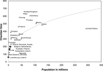
Taagepera's cube-root equation has been accurate in estimating the legislature size-to-population ratio for most advanced democracies. Figure 3 plots the population of all of the countries from the Organization of Economic Co-operation and Development (OECD), the size of their lower chambers, and a cube-root trend line.69
The data are from the 2004 U.S. Central Intelligence Agency's Factbook. See https://www.cia.gov/cia/publications/factbook/.
The ten worse negatively apportioned lower chambers belong, in descending order, to: India, United States, Bangladesh, Pakistan, Philippines, Columbia, Peru, Saudi Arabia, Kazakhstan, and Nigeria. The lower chamber's membership size is not the most important issue determining the quality of representation in many of these countries.

Populations and sizes of lower chamber, OECD countries
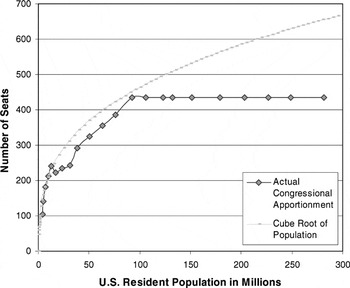
The history of House membership demonstrates that when Congress adjusted the apportionment size of the House, its size coincidently conformed to the cube-root law. Figure 4 plots the size of the House and the U.S. population after each decennial reapportionment since 1790. Because the U.S. population increased each decade, the plotted points are also in chronological order. Every decade from 1790 to 1910, the House apportionment changed, including a decrease in the House membership size in 1840. These decennial adjustments map closely with the cube root of the U.S. population. In some ways, this endorses the logic inherent in Madison's arguments and in the “cube-root law.” After 1910, the flat line in figure 4 indicates the fixed size of the House membership at 435. The growing discrepancy from the cube root of the U.S. population is apparent: from 1790 to 1910, the House membership size and reapportionment closely followed what today would be consistent with the cube root of the population. Only after 1910 does the apportionment of the U.S. House increasingly diverge from its historical tradition and the present practice of most advanced democracies.

U.S. House apportionment, 1790–2000
Given the uneven distribution of state populations, the territorial basis of congressional representation, and the vexations attendant upon apportioning population remainders, interstate malapportionment will never be absolutely eliminated. A U.S. House apportioned to the cube root of the population, however, would significantly diminish its extent. Figure 5 plots the average state discrepancy (the difference between a state's average district size and the nation's average district size) of all states from 1920 (the first failure to reapportion) through 2000. Negative values indicate overrepresented states; positive values, underrepresented states; and the flat line (at 0) is the national average for each decade. Similar to figure 2, some interstate malapportionment remains. Unlike figure 2, the average district discrepancies for most of the states hew closely to the national district average. The chart, however, may visually underrepresent the change. The current constitutionally accepted measurement standard of one-person, one-vote set by U.S. Commerce v. Montana is the sum of squared difference of each state's average district size from the national average. The cumulative sum of squares from 1920 to 2000 for the 435-members chamber is 1.06 E+12, and the sum of squares for the cube root chamber is 4.32 E+11, a decrease in interstate malapportionment of almost 60 percent.

Interstate malapportionment by state size: 1920–2000 apportioned by cube-root
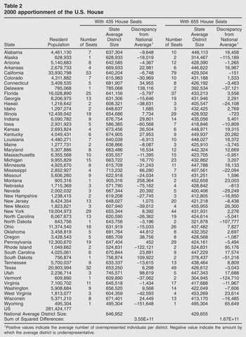
Focusing on the current apportionment, table 2 displays the apportionment population, the average district size, and the average discrepancy between the state and national average district size for all states in a 435-member chamber and a 655-member chamber. The average interstate malapportionment among the states with the greatest discrepancies between each state's average congressional size and the national average in the hypothetical 655-member House (the average would be 67,650 individuals) is reduced by 40 percent compared to the 435-member House. Among the ten states with the smallest discrepancies (the average would be 1,443 individuals), interstate malapportionment is reduced by 65 percent. Among the ten smallest states (the average discrepancy would be 66,080 individuals), it is reduced by 27 percent; and, among the ten largest states (the average discrepancy would be 3,701 individuals), it is reduced by 56 percent.72
The percentages are simply the difference between the 2000 average aggregate discrepancy for each category for the 435-member chamber and the 2000 average aggregate discrepancy for each category for the 655-members chamber, divided by the former.
The sum of squares for the 435-member House is 3.55 E+11; the sum of squares for the 655-member House is 1.67 E+11. The sum of absolute differences (the Dean method) is also reduced (by 30 percent) from 7.56 E+6 to 5.31 E+6.
2000 apportionment of the U.S. House

The decline in interstate malapportionment with a 655-member chamber is in part due to the fact that only one state, Wyoming, would have the minimum of one House member. Although not every state would decrease the discrepancy between its average district population and the national average, the representation of every individual regardless of state residence would become more equal (as measured by the sum of squared differences); the average national district population would decrease from 646,952 to 429,655 individuals; and, most important, one-person, one-vote would be more fully realized. Hence, increasing the membership of the U.S. House of Representatives to the cube root of the U.S. apportionment population in order to aid in remedying interstate malapportionment is a practical and normatively feasible alternative.
This might well have been an advantageous argument for Montana. Perhaps foreseeing the conservative line of reasoning of the Court in U.S. Commerce v. Montana (foreshadowed in Colegrove v. Green in 1946), Montana may have been wise not to argue against the constitutionality of the apportionment method, but rather against the constitutionality of the 1929 Automatic Apportionment Act and the fixed size of House membership.74
Kromkowski and Kromkowski 1991, 135.
Consequences of Increasing the Size of the House
We have identified a significant and serious concern that has received little attention in the popular press and academic literature: interstate malapportionment among U.S. House districts. We have also suggested one possible reform to ameliorate the problem: increasing the size of the House membership to the cube root of the U.S. resident population. Nonetheless, there are naturally more than a few critiques of enlarging the House that are, at the very least, viscerally appealing.75
For instance, do we really want more politicians? Increasing the number of members would also create practical challenges, such as accommodating them within the physical dimensions of the chamber and its offices. A larger House membership might mitigate malapportionment at the expense of greater political acrimony.76 Or, because a larger membership would diminish the relative strength of each individual member, would it not make such a reform unlikely to pass? There is no way conclusively to rebut these and other critiques.77Kromkowski and Kromkowski 1991 list twenty-five possible benefits that, for the most part, add to the benefits discussed here.
Notwithstanding that interstate malapportionment presents serious constitutional, normative, and practical concerns, which undermine the political equality and fairness that define the standards of American democracy and representation, increasing the size of House membership is the only feasible alternative reform that would have a significant impact on the population discrepancies without amending the Constitution. Furthermore, minimizing interstate malapportionment by increasing the size of House membership could have additional positive effects throughout the federal system.
Apportionment can have considerable distribution consequences.78
Kromkowski 2002, xvii.
Cho 1976, 71.
If the rural/urban divide corresponds with partisan preferences—as Lang and Sanchez argue—the effects of malapportionment are not limited to Congress and the distribution of federal funds.81
Lang and Sanchez 2006.
This result is based on the assumption that Bush won Florida; all of the districts of Maine and Nebraska still voted for Gore and Bush, respectively; and that Washington, D.C. only has three electoral votes. Washington, D.C. had a population of 606,900 in the 1990 U.S. Census. This amount is large enough to have earned two “ghost” members in the U.S. House and thus four Electoral College votes. However, the Twenty-Third Amendment to the Constitution states that the number of electors assigned to Washington, D.C. should “in no event [be] more than the least populous State.” Because Alaska and Wyoming still would have had three electoral votes, so would the District.
Neubauer and Zeitlin 2003.
An increase in the membership of the House could have other positive externalities as well, such as increasing the likelihood that more African-Americans, Hispanics, and women would be elected.84
Darcy and Choike 1986.
Leib and Webster 1997.
Canon 1999.
Mansbridge 1999.
Kromkowski and Kromkowski 1991, 143.
Further, the relationship between the number of votes a political party receives and the number of seats that it wins varies with the size of the legislative chamber.89
The smaller the chamber, the more the majority party will be disproportionally overrepresented. For example, in a chamber of one seat, the candidate receiving the plurality of votes wins all of the seats while the candidate(s) receiving less than a plurality of votes wins no seats. Lucas and McDonald argue that because single-member districts have been assumed to produce a votes-to-seats ratio close to the cube-root law, the House should be reapportioned to the cube root of the U.S. population.90Lucas and McDonald 2000, 377.
Bond and Fleisher 2000.
Lucas and McDonald 2000, 377–78.
Conclusion
During the 1960s, the Supreme Court took aim at a highly undemocratic form of disenfranchisement: intrastate malapportionment. It did so with a doctrine that underscores the recognition of the essential equality of every individual required by the U.S. Constitution and, more generally, representative democracy. Today, however, the problematic effects of another type of malapportionment, interstate malapportionment, rarely are discussed. Unlike the sets of undemocratic intentions and conditions that triggered the Court's original intervention, the causes of contemporary interstate malapportionment are more difficult to attribute to nefarious intentions. Instead, the causes are the uneven distribution of state populations; the territorially-based House districts; the apportionment method; and the fixed and limited House membership. Nonetheless, interstate malapportionment should be considered no less significant than intrastate malapportionment. The presence of systematic and disproportional interstate malapportionment poses serious constitutional, normative, and practical problems, which warrant appreciably greater consideration. We suggest that increasing House membership from its current size of 435 to the cube root of the nation's resident population is the only feasible alternative procedural remedy that more fully achieves the current principles, interpretations, and standards of the Constitution.
Our suggestion is made with due caution and the recognition that “no political problem is less susceptible of a precise solution than that which relates to the number most convenient for a representative legislature.”93
Madison, Federalist No. 55, in Kesler and Rossiter, eds., 1999, 309.
Moscardelli and Haspel 2007.