2.1. An extension of K41 by the idea of LRT

In the study of TSF, it is common practice to decompose the filed ${\tilde {{\boldsymbol {u}}}}$ into a mean ${\boldsymbol {U}}$ and fluctuating part ${\boldsymbol {u}}$ such that ${\tilde {{\boldsymbol {u}}}}={\boldsymbol {U}}+{\boldsymbol {u}}$. Corresponding to this decomposition, ${\tilde {{\boldsymbol {v}}}}$ defined by (2.3) can be decomposed as

(2.4)\begin{equation} {\tilde{{\boldsymbol{v}}}}={\tilde{{\boldsymbol{v}}}}({\boldsymbol{r}},s)= {\boldsymbol{V}}({\boldsymbol{r}},s)+{\boldsymbol{v}}({\boldsymbol{r}}, s), \end{equation}

where

(2.5)\begin{gather} {\boldsymbol{V}}={\boldsymbol{V}}({\boldsymbol{r}},s)= {\boldsymbol{U}}({\boldsymbol{r}} +{\boldsymbol{r}}_0,s+t_0) -{\boldsymbol{U}}({{\boldsymbol{x}}}_0, t_0), \end{gather}

(2.6)\begin{gather} {\boldsymbol{v}}={\boldsymbol{v}}({\boldsymbol{r}},s)= {\boldsymbol{u}}({\boldsymbol{r}} +{\boldsymbol{r}}_0, s+t_0)-{\boldsymbol{u}}({{\boldsymbol{x}}}_0, t_0). \end{gather}

In the frame $\mathcal {F}$, we have

(2.7)\begin{equation} \frac{\partial}{\partial s} {{\boldsymbol{v}}}={-}({\boldsymbol{V}}\boldsymbol{\cdot} \boldsymbol{\nabla}){ {\boldsymbol{v}}}- ({\boldsymbol{v}} \boldsymbol{\cdot}\boldsymbol{\nabla}) {\boldsymbol{V}} - ({{\boldsymbol{v}}} \boldsymbol{\cdot} {\boldsymbol{\nabla}}) {{\boldsymbol{v}}} +\left\langle ({{\boldsymbol{v}}} \boldsymbol{\cdot} {\boldsymbol{\nabla}}) {{\boldsymbol{v}}} \right\rangle -\frac{1}{\rho } \boldsymbol{\nabla} p+ \nu \nabla^2 {\boldsymbol{v}} - \boldsymbol{R}, \end{equation}

for the fluctuating field $({\boldsymbol {v}},p)$, where $p\equiv {\tilde {p}}-\left \langle p \right \rangle$, $\boldsymbol{R}\equiv (\boldsymbol{u}(\boldsymbol{x}_0,t_0)\cdot \boldsymbol{\nabla}) \boldsymbol{V}$, $\boldsymbol {\nabla }=(\partial /\partial x_1, \partial /\partial x_2, \partial /\partial x_3)= (\partial /\partial r_1, \partial /\partial r_2, \partial /\partial r_3)$, and $a_i$ is the ith Cartesian component of vector $\boldsymbol{a}$.

In this subsection, we propose an extension of K41 on the basis of the application of the idea of the LRT. The application is based on rough estimates of terms in (2.7) for eddies of scales $\sim \eta$. As seen below, the estimates can be obtained in a simple way similar to those presented in studies including e.g. Kaneda & Yoshida (Reference Kaneda and Yoshida2004), Kaneda (Reference Kaneda2020), which give estimates for eddies of scales $\ll L_U$, in the context of the applications of the idea of LRT to turbulent flows, where $L_U$ is the characteristic length scale of ${\boldsymbol {U}}$.

Since at time $t=t_0$, i.e. $s=0$, ${\boldsymbol {V}}$ can be expanded for $r \equiv |{\boldsymbol {r}}| \ll L_U$ as

(2.8) \begin{equation} \boldsymbol{V}=\boldsymbol{U}({\boldsymbol{r}}+{\boldsymbol{x}}_0,t_0)-\boldsymbol{U}({\boldsymbol{x}}_0,t_0) = \frac{\partial \boldsymbol{U}}{\partial x_\alpha}r_\alpha +\cdots, \end{equation}

we have at the time instant $s=0$,

(2.9) \begin{equation} ({\boldsymbol{V}} \boldsymbol{\cdot} \boldsymbol{\nabla}){ {\boldsymbol{v}}} + ({\boldsymbol{v}} \boldsymbol{\cdot}\boldsymbol{\nabla}) {\boldsymbol{V}}= \left( \frac{\partial U_\alpha}{\partial x_\beta} r_\beta \right) \frac{\partial \boldsymbol{v}}{\partial r_\alpha} + v_\alpha \frac{\partial \boldsymbol{U}}{\partial x_\alpha} + \cdots, \end{equation}

for $r \ll L_U$, where the summation convention is used for repeated Greek indices, $\partial U_i/{\partial x_j}$ are the mean flow gradients at ${\boldsymbol {x}}={\boldsymbol {x}}_0$, i.e. they are ${\partial U_{i}}/{\partial x_j}|_{{\boldsymbol {x}}={\boldsymbol {x}}_0}$ and we omit the symbol ‘$|_{{\boldsymbol {x}}={\boldsymbol {x}}_0}$’ for ease of writing, and we have used $\partial u_i/\partial x_j=\partial v_i/\partial r_j$. We assume time dependence of ${\boldsymbol {U}}$ to be negligible in the following. We also assume that $L_U$ is so large that the gradients of $\boldsymbol {R}$ in (2.7) are sufficiently small, i.e. $\boldsymbol{R}$ is almost constant in the domain $r \ll L_U$, and therefore $\boldsymbol{R}$ is negligible in considering the small-scale statistics, such as those of velocity differences between two points, in the domain.

Rough order estimates of the first three terms on the right-hand side of (2.7) and the terms in (2.9) for $r \sim \eta$ can be obtained by putting ${\boldsymbol {v}} \sim v_\eta$, $\boldsymbol{\nabla} \boldsymbol{v} \sim v_\eta/\eta$ and $\nabla^2 \boldsymbol{v} \sim v_\eta/\eta^2$, where $\eta$ is the Kolmogorov length scale given by $\eta =(\nu ^3/\left \langle \epsilon \right \rangle )^{1/4}$, $v_\eta$ is the characteristic velocity scale of eddies of scales $\sim \eta$ and given by $v_\eta \sim (\left \langle \epsilon \right \rangle \nu )^{1/4}$, $\epsilon$ is the local rate of the energy dissipation per unit mass that is due to solely the fluctuating part $\boldsymbol{u}$ and defined independently of the mean flow $\boldsymbol{U}$ ($\epsilon$ is simply called the energy dissipation rate in the following) and the symbol ‘$\sim$’ denotes equality in the order of magnitude. Then, we obtain

(2.10) \begin{gather} \left( \frac{\partial U_\alpha}{\partial x_\beta} r_\beta \right) \frac{\partial \boldsymbol{v}}{\partial r_\alpha} + v_\alpha \frac{\partial \boldsymbol{U}}{\partial x_\alpha} \sim S v_\eta =S(\left\langle \epsilon \right\rangle \nu)^{1/4}, \end{gather}

(2.11)\begin{gather} ({{\boldsymbol{v}}} \boldsymbol{\cdot} {\boldsymbol{\nabla}}) {{\boldsymbol{v}}} \sim \frac{v_\eta^2}{\eta} = \left( \frac{\left\langle \epsilon \right\rangle ^3}{\nu} \right)^{1/4}, \end{gather}

and

(2.12)\begin{equation} \nu \nabla^2 {\boldsymbol{v}} \sim \frac{\nu v_\eta}{\eta^2}= \left( \frac{\left\langle \epsilon \right\rangle ^3}{\nu}\right)^{1/4}, \end{equation}

where $S$ is an appropriate norm of the tensor $(\partial U_i/\partial x_j)$ such as $[(\partial U_\alpha /\partial x_\beta )(\partial U_\alpha /\partial x_\beta )]^{1/2}$, and it is assumed that $\eta \ll L_U$ and $L$.

Equations (2.10)–(2.12) give

(2.13)\begin{equation} ({\boldsymbol{V}} \boldsymbol{\cdot} \boldsymbol{\nabla}){ {\boldsymbol{v}}} + ({\boldsymbol{v}} \boldsymbol{\cdot}\boldsymbol{\nabla}) {\boldsymbol{V}} \sim \gamma [ ({{\boldsymbol{v}}} \boldsymbol{\cdot} {\boldsymbol{\nabla}}) {{\boldsymbol{v}}} ] \sim \gamma [ \nu \nabla^2 {\boldsymbol{v}}] , \end{equation}

where $\gamma$ is the ratio of the time scale $\tau _\eta \equiv \eta /v_\eta$ of small eddies of size $\sim \eta$ to the time scale $\tau _S \equiv 1/S$ associated with the mean shear,

(2.14)\begin{equation} \gamma \equiv \frac{\eta/v_\eta}{1/S}= S \frac{\eta}{v_\eta} =\frac{S(\left\langle \epsilon \right\rangle \nu)^{1/4}}{ (\left\langle \epsilon \right\rangle ^3/\nu)^{1/4}}=S\left( \frac{\nu}{\left\langle \epsilon \right\rangle }\right)^{1/2}. \end{equation}

Equation (2.13) implies that $\gamma$ may be interpreted not only as the time ratio $\tau _\eta /\tau _S$, but also as the time ratio $\tau _N/\tau _S$ for eddies of scales $\sim \eta$, where $\tau _N$ is the characteristic time scale associated with the convection term $({{\boldsymbol {v}}} \boldsymbol {\cdot } {\boldsymbol {\nabla }}) {{\boldsymbol {v}}}$.

Equation (2.13) also implies that if

(2.15)\begin{equation} \gamma \equiv S\left( \frac{\nu}{\left\langle \epsilon \right\rangle }\right)^{1/2} \ll 1, \end{equation}

then the magnitude of the first two terms on the right-hand side of (2.7), i.e. the terms representing the direct coupling between ${\boldsymbol {v}}$ and the mean flow ${\boldsymbol {V}}$, is negligibly small compared with that of the nonlinear coupling term $({{\boldsymbol {v}}}\boldsymbol {\cdot } {\boldsymbol {\nabla }}) {{\boldsymbol {v}}}$ and the viscous term $\nu \nabla ^2 {\boldsymbol {v}}$. This suggests that, if $\gamma \ll 1$, then the influence of the two terms on the distribution law of probabilities $F_n$ for $r \sim \eta$, is negligibly small compared with those of $({{\boldsymbol {v}}}\boldsymbol {\cdot } {\boldsymbol {\nabla }}) {{\boldsymbol {v}}}$ and $\nu \nabla ^2 {\boldsymbol {v}}$. If the two terms and $\boldsymbol{R}$ can be ignored, then the equation of motion (2.7) is compatible with isotropy, i.e. invariant to arbitrary rotation of the coordinate system.

(Note: by comparing the characteristic inertial transfer time scale and the time scale ($\sim 1/S$) associated with the mean shear in the wavenumber range $\sim k$, and by using the ISR energy spectrum given by K41, Corrsin (Reference Corrsin1958) argued that

(2.16)\begin{equation} k^{2/3} \gg \left\langle \epsilon \right\rangle ^{{-}1/3} S \end{equation}

need be satisfied for the local isotropy of the statistics in the wavenumber range $\sim k$ in the ISR of TSF. Here, we are ignoring constants of order unity. If we put $k \sim 1/\eta$, then (2.16) gives (2.15). In terms of length scales, the inequalities (2.15) and (2.16) are respectively equivalent to $\eta /L_C \ll 1$ and $\ell /L_C \ll 1$ with $\ell \sim 1/k$, where $L_C$ is Corrsin's length scale given by $L_C=(\left \langle \epsilon \right \rangle /S^3)^{1/2}$.)

These observations suggest to us to exploit the idea of LRT of turbulence. LRT is based on the assumption of the existence of a certain kind of equilibrium state under certain conditions. Suppose that a disturbance, say $X$, is added to a system that is in an equilibrium state in the absence of $X$. Then, in response to this disturbance, the statistical average $\left \langle B \right \rangle$ of observable $B$ changes from $\left \langle B \right \rangle _e$ to

(2.17)\begin{equation} \left\langle B \right\rangle= \left\langle B \right\rangle _e + \Delta \left\langle B \right\rangle, \end{equation}

where $\left \langle B \right \rangle _e$ is the average in the equilibrium state in the absence of $X$, and $\Delta \left \langle B \right \rangle$ denotes the change owing to $X$. In LRT, it is assumed that if $X$ is appropriately small, then $\Delta \left \langle B \right \rangle$ can be approximated to be the first order in $X$, i.e.

(2.18)\begin{equation} \Delta \left\langle B \right\rangle= \Delta_1\left\langle B \right\rangle + \cdots, \end{equation}

where $\Delta _1 \left \langle B \right \rangle$ denotes a first-order term in $X$ and ‘$\cdots$’ denotes higher-order terms in $X$; $\Delta _1 \left \langle B \right \rangle$ can be written as

(2.19)\begin{equation} \Delta_1 \left\langle B \right\rangle= c X, \end{equation}

in which X is to be understood as a measure representing the disturbance in an appropriate sense, and $c$ is a coefficient determined by the nature of the equilibrium state, independently of $X$. If the disturbance consists of more than one type of disturbance, $X_1, X_2, \ldots$, (2.19) is to be understood as

(2.20)\begin{equation} \Delta_1 \left\langle B \right\rangle= c_1X_1+c_2X_2 +\cdots, \end{equation}

where $c_1$ and $c_2$ are constants. Readers may refer to Kaneda (Reference Kaneda2020) for some details on the idea of LRT applied to turbulent flows.

In accordance with K41, we assume here that, in the limit of small $\gamma$, the turbulence domain $G$ under consideration is in a locally isotropic equilibrium state satisfying the first hypothesis of similarity, and we apply the idea of LRT to estimate the influence of small but finite $\gamma$ on the statistics at small scales $\sim \eta$ in TSF. Let $B$ be an observable whose average is dominated by the statistics at scales $r \sim \eta$. We assume the following three hypotheses.

1. (i) The first hypothesis of similarity for TSF.

   In the limit $\gamma \to 0$, the statistics of $B$ are locally isotropic, and the average $\left \langle B \right \rangle$ is uniquely determined by $\nu$ and the local quantity $\left \langle \epsilon \right \rangle$ independently of the mean flow gradients $\partial U_i/\partial x_j$.

Regarding the effect of small but finite $\gamma$:

1. (ii) The second hypothesis of similarity for TSF.

   For sufficiently small but finite $\gamma$, the change $\Delta \left \langle B \right \rangle$ of $\left \langle B \right \rangle$ owing to the mean shear can be approximated to be linear in $\gamma$, i.e. $\Delta \left \langle B \right \rangle \approx \Delta _1 \left \langle B \right \rangle$, where $\Delta _1 \left \langle B \right \rangle = c \gamma$, in which the coefficient $c$ is independent of $\gamma$.

2. (iii) The third hypothesis of similarity for TSF.

   The coefficient $c$ is uniquely determined by the locally isotropic equilibrium state in the absence of mean shear, so that it is uniquely determined by $\nu$ and the local quantity $\left\langle\epsilon \right\rangle$.

In the context considering the dependence of statistics on $\gamma$ at small $\gamma$, the symbol ‘$\approx$’ denotes equality in the sense of neglecting terms of order higher in $\gamma$ than that (those) of the retained term(s).

The local equilibrium state assumed in K41 and the first hypothesis of similarity for TSF can in general be disturbed not only by the mean shear, but also by other effects such as the anisotropy in energy-containing eddies and inhomogeneity of the pressure field due to the existence of the boundary wall. Regarding the influence of anisotropy in energy-containing eddies, see the discussions in § 4.1. The main interest of this study is the influence of the mean shear, and it is assumed that the other effects, if there are any, on the statistics at scales $\sim \eta$ are insignificant or at most of an order of magnitude similar to that of the effect of the mean shear. LRT suggests that if such other effects are not negligible, then one may add their influence as in (2.20), provided that they are small in an appropriate sense.

2.2. Application to the statistics of velocity gradients

Let $g_{ij}$ be the gradient of the fluctuating velocity field given by

(2.21)\begin{equation} g_{ij}\equiv g_{ij} ({\boldsymbol{x}},t) \equiv \frac{\partial u_i}{\partial x_j}= \frac{\partial v_i}{\partial r_j}. \end{equation}

It is natural to assume that the $p$th-order moments $\left \langle g_{ij}g_{mn}\cdots \right \rangle$ are dominated by the statistics of small eddies in the energy dissipation scale range. The application of the first hypothesis of similarity for TSF to $B=g_{ij}g_{mn}\cdots$ then gives the following for $p$th-order moments

(2.22)\begin{equation} \left\langle g_{ij}g_{mn}\cdots \right\rangle \to \left\langle g_{ij}g_{mn}\cdots \right\rangle_e = f^{(\,p)}_{ijmn\ldots}(\nu, \left\langle \epsilon \right\rangle ), \end{equation}

in the limit of sufficiently small $\gamma$, where $f^{(\,p)}_{ijmn\ldots }$ is an appropriate isotropic tensor depending only on $\nu$ and local average $\left \langle \epsilon \right \rangle$ at position ${\boldsymbol {x}}$. A dimensional consideration gives

(2.23)\begin{equation} \left\langle g_{ij}g_{mn}\cdots \right\rangle_e= \left( \frac{\left\langle \epsilon \right\rangle }{\nu} \right)^{p/2} C^{(\,p)}_{e,ijmn\cdots}, \end{equation}

where $C^{(\,p)}_{e,ijmn\cdots }$ are dimensionless $2p$th-order isotropic tensors. If $\gamma$ is small but finite, then $\left \langle g_{ij}g_{mn}\cdots \right \rangle$ generally change from $\left \langle g_{ij}g_{mn}\cdots \right \rangle _e$ to

(2.24)\begin{equation} \left\langle g_{ij}g_{mn}\cdots \right\rangle = \left\langle g_{ij}g_{mn}\cdots \right\rangle_e + \Delta \left\langle g_{ij}g_{mn}\cdots \right\rangle, \end{equation}

where 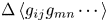$\Delta \left \langle g_{ij}g_{mn}\cdots \right \rangle$ are the changes due to the disturbance by the small but finite mean shear, represented by $\gamma$. The second hypothesis of similarity for TSF implies that $\Delta \left \langle g_{ij}g_{mn}\cdots \right \rangle$ can be approximated to be linear in $\gamma$, so that

(2.25)\begin{equation} \Delta \left\langle g_{ij}g_{mn}\cdots \right\rangle \approx \Delta_1 \left\langle g_{ij}g_{mn}\cdots \right\rangle = c^{(\,p)}_{1,ijmn \ldots} \gamma, \end{equation}

in which the coefficients $c^{(\,p)}_{1,ijmn \ldots }$ are independent of $\gamma$. The third hypothesis of similarity for TSF implies that the coefficients $c_{1,ijmn \cdots }$ depend only on $\left \langle \epsilon \right \rangle$ and $\nu$. A dimensional consideration then gives

(2.26)\begin{equation} \Delta_1 \left\langle g_{ij}g_{mn}\cdots \right\rangle = \gamma \left( \frac{\left\langle \epsilon \right\rangle }{\nu}\right)^{p/2} C^{(\,p)}_{1,ijmn\cdots}, \end{equation}

where $C^{(\,p)}_{1,ijmn\cdots }$ are dimensionless constants.

From (2.23)–(2.26), we have for $p=2$,

(2.27)\begin{equation} \left\langle g_{ij}g_{mn} \right\rangle \approx \left\langle g_{ij}g_{mn} \right\rangle _e + \Delta_1 \left\langle g_{ij}g_{mn} \right\rangle = \frac{\left\langle \epsilon \right\rangle }{\nu} \left(C_{e,ijmn}+\gamma C_{1,ijmn}\right), \end{equation}

where $C_{e,ijmn}$ and $C_{1,ijmn}$ are dimensionless constants independent of $\nu , \left \langle \epsilon \right \rangle$ and $S$, and superscript ‘$(2)$’ is omitted for simplicity. The second hypothesis of similarity for TSF implies that $C^{(\,p)}_{1,ijmn\ldots }$ are dimensionless constant tensors that are independent of the norm $S$, but it does not exclude the possibility of the dependence of $C_{1,ijmn}$ on components $(\partial U_i/\partial x_j)/S$. (See discussions in § 4.2.)

Since $C_{e,ijmn}$ is a fourth-order isotropic tensor, it may be written without loss of generality as

(2.28)\begin{equation} C_{e,ijmn} =a \delta_{ij}\delta_{mn} + b \delta_{im}\delta_{jn} + c \delta_{in}\delta_{jm}, \end{equation}

where $a,b$ and $c$ are dimensionless constants that are independent of $\left \langle \epsilon \right \rangle$ and $\nu$. (This $c$ is to be not confused with $c$ in the other contexts such as in (2.19).) Since $g_{\alpha \alpha }=0$ due to the incompressibility condition, we have $C_{e,\alpha \alpha m n}=0$ for any $m,n$, so that

(2.29)\begin{equation} C_{e,\alpha\alpha mn} =3a\delta_{mn} + b \delta_{mn} + c \delta_{mn}=0, \end{equation}

i.e.

(2.30)\begin{equation} 3a+b+c=0. \end{equation}

If the flow statistics are homogeneous in two Cartesian directions, say in the $x_1$- and $x_3$-directions, then

(2.31)\begin{align} \left\langle g_{13}g_{31}\right\rangle-\left\langle g_{11}g_{33}\right\rangle &=\left\langle \frac{\partial u_1}{\partial x_3}\frac{\partial u_3}{\partial x_1}\right\rangle - \left\langle \frac{\partial u_1}{\partial x_1}\frac{\partial u_3}{\partial x_3}\right\rangle \nonumber\\ &= \frac{\partial }{\partial x_3} \left\langle u_1\frac{\partial u_3}{\partial x_1}\right\rangle- \frac{\partial }{\partial x_1} \left\langle u_1\frac{\partial u_3}{\partial x_3}\right\rangle=0. \end{align}

Equation (2.31) implies $C_{e,1331}=C_{e,1133}$, so that we have $c=a$ from (2.28) (cf. Kida & Orszag (Reference Kida and Orszag1990)). Then, (2.30) gives $b=-4a$, so that (2.28) can be reduced to

(2.32)\begin{equation} C_{e,ijmn} =a \left( \delta_{ij}\delta_{mn} -4 \delta_{im}\delta_{jn} + \delta_{in}\delta_{jm} \right). \end{equation}

Because

(2.33)\begin{equation} \epsilon= 2\nu s_{\alpha\beta}s_{\alpha\beta}, \end{equation}

in which $s_{ij}=(g_{ij}+g_{ji})/2$, we have $\left \langle \epsilon \right \rangle /\nu = \left \langle (g_{\alpha \beta }+g_{\beta \alpha }) g_{\alpha \beta }\right \rangle$. Therefore, (2.27) yields $C_{e,\alpha \beta \alpha \beta }=1$. Thus (2.32) gives

(2.34)\begin{equation} a={-}\tfrac{1}{30} \end{equation}

(see § 3.1). Note that statistical homogeneity in the $x_2$-direction is not assumed in the derivation of (2.32), but (2.32) is still the same as the well-known expression for $\left \langle g_{ij}g_{mn} \right \rangle$ in homogeneous and isotropic turbulence (cf. e.g. Hinze Reference Hinze1975; Kida & Orszag Reference Kida and Orszag1990; Pumir Reference Pumir2017).

Equations (2.27), (2.32) and (2.34) give among others

(2.35)\begin{gather} \frac{\nu}{\left\langle \epsilon \right\rangle } \left\langle \left( \frac{\partial u_i}{\partial x_i}\right)^2 \right\rangle =\frac{\nu}{\left\langle \epsilon \right\rangle } \left\langle g_{ii}g_{ii}\right\rangle \approx \frac{1}{15}+ \gamma C_{1, iiii} , \end{gather}

(2.36)\begin{gather} \frac{\nu}{\left\langle \epsilon \right\rangle } \left\langle \left( \frac{\partial u_i}{\partial x_j}\right)^2 \right\rangle =\frac{\nu}{\left\langle \epsilon \right\rangle } \left\langle g_{ij}g_{ij}\right\rangle \approx \frac{2}{15}+ \gamma C_{1, ijij} , \end{gather}

(2.37)\begin{gather} \frac{\nu}{\left\langle \epsilon \right\rangle } \left\langle \frac{\partial u_i}{\partial x_j}\frac{\partial u_k}{\partial x_j}\right\rangle =\frac{\nu}{\left\langle \epsilon \right\rangle } \left\langle g_{ij}g_{kj}\right\rangle \approx \gamma C_{1, ijkj}, \end{gather}

and

(2.38)\begin{equation} \frac{\left\langle \left( {\partial u_i}/{\partial x_j}\right)^2 \right\rangle} {\left\langle \left( {\partial u_i}/{\partial x_i}\right)^2 \right\rangle} = \frac{\left\langle g_{ij}g_{ij} \right\rangle}{ \left\langle g_{ii}g_{ii} \right\rangle} \approx 2+ \gamma( 15C_{1,ijij}-30C_{1,iiii}), \end{equation}

where $i \ne j$, $i \ne k$, no summation is taken over repeated italic indices and in (2.37) we have used $C_{e,ijkj}=0$ because of (2.32).

Equations (2.27), (2.32) and (2.34) also give

(2.39)\begin{equation} \frac{\nu}{\left\langle \epsilon \right\rangle } \left\langle \frac{\partial u_i}{\partial x_\alpha }\frac{\partial u_j}{\partial x_\alpha} \right\rangle =\frac{\nu}{\left\langle \epsilon \right\rangle } \left\langle g_{i\alpha}g_{j\alpha}\right\rangle =\frac{\epsilon_{ij}}{2\left\langle \epsilon \right\rangle } \approx \frac{1}{3} \delta_{ij} + \gamma C_{1, i\alpha j\alpha } , \end{equation}

where $\epsilon _{ij}$ is defined by $\epsilon _{ij} \equiv 2\nu \left \langle g_{i\alpha }g_{j\alpha } \right \rangle$, and we used $C_{e, i\alpha j\alpha }=(1/3)\delta _{ij}$.

Constants $1/15, 2/15, 2$ and $1/3$ on the right-hand side of (2.35), (2.36), (2.38) and (2.39) are derived from the isotropic tensor $C_{e,ijmn}$ given by (2.32) with (2.34), i.e. they agree with the results obtained by ignoring the anisotropy of statistics.

2.3. Statistics in the inertial sublayer of the turbulent boundary layer

It is known that in a turbulent boundary layer with mean flow ${{\boldsymbol {U}}}=(U_1,U_2,U_3) \equiv \left \langle {\tilde {{\boldsymbol {u}}}} \right \rangle =(U(y),0,0)$ at sufficiently large $Re_\tau$ and $y^+$, there is flow region called the inertial sublayer in which the mean flow $U(y)$ is approximately given by

(2.40)\begin{equation} \left( \frac{\textrm{d}U}{\textrm{d}y} \right)^+{\approx} \frac{1}{ \kappa y^+}, \end{equation}

where the coefficient $\kappa$ is a dimensionless constant known as the constant of von Kármán, $y$ is the distance from the wall, symbol $^+$ denotes the normalisation by the wall-friction velocity given by $u_\tau ^2=\nu (\textrm {d}U/{\textrm {d}y})|_{y=0}$ and the wall-friction length is defined by $\ell _\tau =\nu/u_\tau$. The friction Reynolds number $Re_\tau$ is given by $Re_\tau \equiv u_\tau \delta /\nu$, where $\delta$ is the channel half-width. In this study, we use ${{\boldsymbol {x}}}=(x_1,x_2,x_3)=(x,y,z)$, and we assume $(\textrm {d}U/{\textrm {d}y})>0$ unless otherwise stated.

It is also known that the mean energy dissipation rate $\left \langle \epsilon \right \rangle$ in the inertial sublayer is approximately given by

(2.41)\begin{equation} \left\langle \epsilon \right\rangle ^+{\approx} \frac{1}{ \kappa_\epsilon y^+}, \end{equation}

where $\kappa _\epsilon$ is a dimensionless constant (see the discussion in § 3.2). If $-\left \langle u_1u_2 \right \rangle \approx (u_\tau )^2$ and if the turbulence production rate $-\left \langle u_1u_2 \right \rangle \, \textrm {d}U/{\textrm {d}y}$ is mainly balanced by the mean energy dissipation rate $\left \langle \epsilon \right \rangle$ in the inertial sublayer, then we have (2.41) with $\kappa _\epsilon =\kappa$ (see e.g. Tennekes & Lumley Reference Tennekes and Lumley1972).

In such a layer, we have

(2.42)\begin{equation} \gamma = S\left( \frac{\nu}{\left\langle \epsilon \right\rangle }\right)^{1/2} \approx K (y^+)^{{-}1/2}, \quad \left( K \equiv \frac{\kappa_\epsilon^{1/2}}{\kappa} \right), \end{equation}

and

(2.43)\begin{equation} \eta^+{\equiv} \left[ \left( \frac{\nu^3}{\left\langle \epsilon \right\rangle } \right)^{1/4} \right]^+{\approx} (\kappa_\epsilon y^+)^{1/4}, \end{equation}

where $\textrm {d}U/{\textrm {d}y}$ is used as the norm $S$ of the gradient tensor $(\textrm {d}U_i/\textrm {d}x_j )$ of the mean velocity.

Substitution of (2.42) into (2.35)–(2.39) gives

(2.44)\begin{gather} \frac{\nu}{\left\langle \epsilon \right\rangle } \left\langle \left( \frac{\partial u_i}{\partial x_i} \right)^2 \right\rangle =\frac{\nu}{\left\langle \epsilon \right\rangle }\left\langle g_{ii}g_{ii} \right\rangle \approx \frac{1}{15} + C_{1, iiii }\times K \times (y^+)^{{-}1/2}, \end{gather}

(2.45)\begin{gather} \frac{\nu}{\left\langle \epsilon \right\rangle } \left\langle \left( \frac{\partial u_i}{\partial x_j}\right)^2 \right\rangle =\frac{\nu}{\left\langle \epsilon \right\rangle }\left\langle g_{ij}g_{ij} \right\rangle \approx \frac{2}{15} + C_{1, ijij } \times K \times (y^+)^{{-}1/2}, \end{gather}

(2.46)\begin{gather} \frac{\nu}{\left\langle \epsilon \right\rangle } \left\langle\frac{\partial u_i}{\partial x_j}\frac{\partial u_k}{\partial x_j}\right\rangle =\frac{\nu}{\left\langle \epsilon \right\rangle }\left\langle g_{ij}g_{kj} \right\rangle \approx C_{1,ijkj} \times K \times (y^+)^{{-}1/2}, \end{gather}

(2.47)\begin{gather} \frac{\left\langle \left({\partial u_i}/{\partial x_j}\right)^2 \right\rangle} {\left\langle \left( {\partial u_i}/{\partial x_i}\right)^2 \right\rangle} = \frac{\left\langle g_{ij}g_{ij} \right\rangle}{\left\langle g_{ii}g_{ii} \right\rangle} \approx 2+ (15 C_{1,ijij}-30C_{1,iiii}) \times K \times (y^+)^{{-}1/2} , \end{gather}

and

(2.48)\begin{equation} \frac{\epsilon_{ij}}{2\left\langle \epsilon \right\rangle } \approx \frac{1}{3}\delta_{ij} + C_{1, i\alpha j\alpha } \times K \times (y^+)^{{-}1/2}, \end{equation}

to the leading order of small $1/y^+$; higher-order terms in $1/y^+$ are omitted in (2.44)–(2.48).

3.1. Data resources

Our statistical analysis was based on a database, which we call DB-TCF, produced from a series of DNSs of TCF with friction Reynolds numbers $Re_\tau$ up to approximately $8000$. The DNSs use a Fourier-spectral method in the wall-parallel, i.e. $x$- and $z$-directions, and a second-order accurate finite-difference method in the wall-normal, i.e. $y$ direction. Alias errors associated with the pseudo-spectral method are removed using the $3/2$ rule. This implies that $(N_x N_z)\times (3/2)^2$ collocation points are used to evaluate the nonlinear convolution terms at each $y$ in the DNSs. Readers may refer to Yamamoto & Kunugi (Reference Yamamoto and Kunugi2011, Reference Yamamoto and Kunugi2016) for the details of the numerical schemes used in the DNSs.

Some of the key DNS parameters are listed in table 1. The initial conditions of R8000 were given by a field generated in a previous DNS (Yamamoto & Tsuji Reference Yamamoto and Tsuji2018) at $Re_\tau \approx 8000$, which used a spatial-resolution and discretisation scheme differing from those of R8000. The statistics of R8000 presented below were obtained from a time interval after a certain initial transient period. In practice, we put the initial transient period of R8000 to be $3Re_\tau$ in wall units. The length of the simulation time interval $7.5 Re_\tau$ in wall units as shown in table 1 is approximately equal to 11.7 $T_w$, where $T_w$ is the wash-out time given by $T_w \equiv L_x/U_c$, in which $U_c$ is the mean centre-line velocity. The statistics of the other runs were also obtained from a time interval (denoted by $T$ in table 1) after a certain initial transient period, which we put to at least $3Re_\tau$ in wall units. It was confirmed that the total shear stress fits the linear profile in all the runs within an error of at most 0.05 in wall units as in previous DNSs (Yamamoto & Tsuji Reference Yamamoto and Tsuji2018). Furthermore, the mean spanwise velocity component normalised by the mean streamwise velocity component is less than 0.07 % at any $y$ in all the runs.

Table 1.

DNS parameters. Here, $U_{b}$ is the bulk velocity, $L_{x}$ and $L_{z}$ are respectively the fundamental periodicity length in the $x$- and $z$-directions, $N_{x}$ ($\Delta x$), $N_{y}$ ($\Delta y$) and $N_{z}$ ($\Delta z$) are respectively the grid numbers (width) in the $x$-,$y$- and $z$-directions, $T$ is the simulation time interval after the initial transient period and $N_{t}$ is the number of flow fields used to compute the second-order moments $\left \langle g_{ij}g_{mn}\right \rangle$ of the fluctuating velocity gradients.

The second-order moments $\left \langle g_{ij}g_{mn} \right \rangle$ of the fluctuating velocity gradients were computed by using several velocity fields stored in the DB-TCF database, and by taking the averages over the homogeneous directions (i.e. the $x$- and $z$-directions) and time. The number of fields is denoted as $N_t$ in table 1. With regards to R4000, such a field is not available in the database, so that no statistics of $\left \langle g_{ij}g_{mn} \right \rangle$ by R4000 are presented below.

Let $\epsilon _g \equiv \nu g_{\alpha \beta } g_{\alpha \beta }$. In homogeneous turbulence, we have $\left \langle \epsilon _g\right \rangle = \left \langle \epsilon \right \rangle$. It is easy to reformulate or re-interpret the theory presented in § 2 using $\epsilon _g$ instead of $\epsilon$. Then, we only need to change appropriately $\epsilon$ to $\epsilon _g$ in and after the first hypothesis of similarity for TSF in § 2. Regarding (2.33), it is to be replaced by $\epsilon _g=\nu g_{\alpha \beta } g_{\alpha \beta }$, but (2.27), (2.32) and (2.34) with $\epsilon$ replaced by $\epsilon _g$ remain valid.

In the analysis of the energy budget in WBT, $\epsilon _g$ plays key roles (see Appendix A), and it is convenient to use $\epsilon _g$ rather than $\epsilon$ as a measure representing the energy dissipation rate. In fact, $\epsilon _g$ has been commonly used in research investigating the WBT budget. The use of $\epsilon _g$ makes it easier for us to compare the DNS results in this study with the reported findings, as shown in figures 2(a) and 2(b) below. In the following in this section and in Appendix A, we therefore use $\epsilon _g$ instead of $\epsilon$ as the measure representing the energy dissipation rate, and we omit the subscript $g$, i.e. we use the symbol $\epsilon _g$ to mean $\nu g_{\alpha \beta } g_{\alpha \beta }$, unless otherwise stated. It is known that the difference between $\left \langle \epsilon \right \rangle$ and $\left \langle \epsilon _g \right \rangle$ is small in WBT for a wide range of Reynolds numbers, at least outside near the wall region (see e.g. Antonia et al. Reference Antonia, Kim and Browne1991; Bradshaw & Perot Reference Bradshaw and Perot1993; Folz & Wallace Reference Folz and Wallace2010; Tardu Reference Tardu2017). This is also confirmed in our DNS results as shown in figure 1. It is unlikely that the difference would significantly affect the discussions in this paper.

Figure 1.

Comparison between $\left \langle \epsilon _g \right \rangle$ and $\left \langle \epsilon \right \rangle$. (a) Distributions of $\left \langle \epsilon _g \right \rangle$ and $\left \langle \epsilon \right \rangle$ and (b) ratio $\left \langle \epsilon _g \right \rangle /\left \langle \epsilon \right \rangle$.

R1000L and R1000H were performed to check the possible influence of spatial resolution on the statistics at the energy DR scales. Although the grid width $\Delta y$ in the wall-normal direction in the runs listed in table 1 is smaller than or similar to $\eta$, those in the wall-parallel directions are larger than $\eta$. Therefore, particular attention was paid to the influence of grid widths $\Delta x$ and $\Delta z$.

Figure 2(a) shows a comparison of $k$-budget terms by R1000L and DNS by Lee & Moser (Reference Lee and Moser2015) at $Re_\tau = 1000$, here $k (= \left \langle u_{\alpha }u_{\alpha } \right \rangle /2)$ is the mean turbulent kinetic energy per unit mass. The grid widths $(\Delta x)^+ = 18.5, (\Delta z)^+ =8.9$ in the former are larger than $(\Delta x)^+ = 10.9, (\Delta z)^+ =4.6$ in the latter. Figure 2(b) shows a comparison of the mean energy dissipation rate ($\left \langle \epsilon \right \rangle$)-budget terms of R1000L and R1000H that is with finer resolution $(\Delta x)^+ = 7.8, (\Delta z)^+ =4.2$. (The data of $\left \langle \epsilon \right \rangle$-budget terms for such a comparison are not available in Lee & Moser Reference Lee and Moser2015.) The definition of the $k$- and $\left \langle \epsilon \right \rangle$-budget terms used in the figures is given in Appendix A ($k$ is not wavenumber in this section nor in Appendix A).

Figure 2.

Grid-sensitivity analysis for R1000L, (a) $k$-budget terms in comparison with DNS by Lee & Moser (Reference Lee and Moser2015), (b) $\left \langle \epsilon \right \rangle$-budget terms in comparison with R1000H.

In both figures 2(a) and 2(b), it is observed that the statistics of R1000L with lower resolution $(\Delta x)^+ = 18.5, (\Delta z)^+ =8.9$ agree well with those of DNSs with higher resolution. The Kolmogorov length scale $\eta$ is generally a function of $Re_\tau$ and $y$. At a given $y$, the scale $\eta$ at higher $Re_\tau$ is similar to $\eta$ at smaller $Re_\tau$ in the region including the inertial sublayer, as shown in Morishita, Ishihara & Kaneda (Reference Morishita, Ishihara and Kaneda2019) and Lee & Moser (Reference Lee and Moser2019). This result and table 1 imply that the grid width in units of $\eta$ of all the runs at $Re_\tau \ge 1000$ listed in table 1 is similar to that in R1000L. The agreement of the $k$- and $\left \langle \epsilon \right \rangle$-budget terms of R1000L with those of DNSs with higher resolution is encouraging for us to use the DNS data for the analysis of the second-order moments of the fluctuating velocity gradients.

3.2. Mean flow, energy dissipation rate and ratio $\gamma$

Figures 3(a) and 3(b) confirm (2.40) and (2.41), where data by DNSs with larger computational domains (Lee & Moser Reference Lee and Moser2015; Hoyas & Jiménez Reference Hoyas and Jiménez2006; Bernardini, Pirozzoli & Orlandi Reference Bernardini, Pirozzoli and Orlandi2014) are also plotted as coloured lines ($\epsilon$ given by (2.33) was used in Bernardini et al. Reference Bernardini, Pirozzoli and Orlandi2014). Figure 3(a) demonstrates that the mean flow profile $U(y)$ fits (2.40) well in a certain range of $y^+$, especially for R8000. Figure 3(b) shows that, although the approximation (2.41) for $\left \langle \epsilon \right \rangle$ is not as good as the approximation (2.40) for $U(y)$, the $y$-dependence of $\left \langle \epsilon \right \rangle y$ in the DNS is fairly weak in that range. In this sense, the results shown in figures 3(a) and 3(b) agree with the observations in Kaneda, Morishita & Ishihara (Reference Kaneda, Morishita and Ishihara2013), Abe & Antonia (Reference Abe and Antonia2016), Morishita et al. (Reference Morishita, Ishihara and Kaneda2019) and Lee & Moser (Reference Lee and Moser2019) (Kaneda et al. (Reference Kaneda, Morishita and Ishihara2013) and Morishita et al. (Reference Morishita, Ishihara and Kaneda2019) used $\epsilon$ given by (2.33)).

Figure 3.

Normalised mean velocity gradient and energy dissipation rate, (a) $(\textrm {d}U^+/{\textrm {d}y}^+)y^+$ vs $y^+$. Thin solid straight lines represent $(\textrm {d}U^+/{\textrm {d}y}^+)y^+$ with $\kappa =0.39$, (b) $\left \langle \epsilon \right \rangle ^+y^+$ vs $y^+$. Thin solid straight lines correspond to $\left \langle \epsilon \right \rangle ^+y^+=1/\kappa _{\epsilon }$ with $\kappa _{\epsilon }=0.45$. Thick straight lines show the ranges $y^+ \in [2.6 Re_\tau ^{1/2}, 0.2Re_{\tau }]$.

Figures 3(a) and 3(b) show that the DNS profiles of $U(y)$ and $\left \langle \epsilon \right \rangle (y)$ depend on $Re_\tau$ and they approach those obtained from simple theories such as (2.40) and (2.41) with an increase in $Re_\tau$. Readers may refer to Jiménez & Moser (Reference Jiménez and Moser2007) and Abe & Antonia (Reference Abe and Antonia2016) for theories on the influence of finite $Re_\tau$ on $U(y)$ and $\left \langle \epsilon \right \rangle (y)$, respectively.

A least squares fit of (2.40) and (2.41) to the DNS data in the range $y^+ \in [2.6 Re_\tau ^{1/2}, 0.2Re_{\tau }]$ (Klewicki Reference Klewicki2010; Chin et al. Reference Chin, Philip, Klewicki, Ooi and Marusic2014) for the run at $Re_\tau \approx 8000$, for which $[2.6 Re_{\tau }^{1/2}, 0.2 Re_{\tau }]\approx [232, 1600]$, gives

(3.1a–c)\begin{equation} \kappa = 0.39, \quad \kappa_{\epsilon} = 0.45, \quad K \equiv \frac{\kappa_\epsilon^{1/2}}{\kappa} = 1.72. \end{equation}

Figure 4(a) plots $\gamma$ as a function of $y^+$ and confirms that, in each run, there is a range of $y$ where $\gamma$ is small. The existence of such a range is a prerequisite for the theory proposed in § 2. In figure 4(b), $\gamma$ in each run is seen to scale well with $(y^+)^{-1/2}$ in an appropriate range, in accordance with (2.42).

Figure 4.

(a) Ratio $\gamma$ vs $y^+$, (b) $y^{+1/2}\gamma$ vs $y^+$. Thin solid straight lines show $\gamma = K(y^+)^{-1/2}$ with $K=1.72$. The meaning of thick straight lines is the same as in figure 3.

3.3. Second-order moments of $g_{ij}$

Figures 5(a,c,e) and 5(b,d,f) show the moments $(\nu /\left \langle \epsilon \right \rangle ) \left \langle g_{ii}^2 \right \rangle$ and the anisotropy correction $| (\nu /\left \langle \epsilon \right \rangle )\left \langle g_{ii}^2 \right \rangle -1/15 |$ for $i, j =1,2$ and $3$, as functions of $y^+$, respectively. Figure 5(a,c,e) displays that, with an increase in $y^+$, i.e. a decrease of $\gamma$, the moments approach the constant $1/15$ in an appropriate range of $y^+$. This is in accordance with (2.44). The slope of anisotropy correction for $i=1$ in figure 5(b,d,f) is approximately $-1/2$, in accordance with (2.44). The slope $-1/2$ for $i=1$ agrees with the value by Lee & Moser (Reference Lee and Moser2019), who computed $(1-15\nu \left \langle g_{11}^2\right \rangle /\left \langle \epsilon \right \rangle )$ and noted that it varies in a manner similar to $(y^+)^{-1/2}$. This slope $-1/2$ for $i=1$ agrees with the value by Lee & Moser (Reference Lee and Moser2019), who computed $(1-15\nu \left \langle g_{11}^2\right \rangle /\left \langle \epsilon \right \rangle )$ and noted that it varies in a manner similar to $(y^+)^{-1/2}$.

Figure 5.

(a,c,e) Value of $\nu \left \langle (g_{ii})^2 \right \rangle /\left \langle \epsilon \right \rangle$ vs $y^+$ for $i=1,2$ and $3$. (b,d,f) The same as (a,c,e) but for $|\nu \left \langle (g_{ii})^2 \right \rangle /\left \langle \epsilon \right \rangle -1/15|$. Thin solid straight lines in (a,c,e) and (b,d,f), respectively, show $\nu \left \langle (g_{ii})^2 \right \rangle /\left \langle \epsilon \right \rangle =1/15$ and the slope $-1/2$. The meaning of thick straight lines is the same as in figure 3.

Figure 5(b,d,f) shows that the moments $(\nu /\left \langle \epsilon \right \rangle ) \left \langle g_{ii}^2 \right \rangle$ for $i=2$ and $3$ approach the isotropy value of $1/15$ with an increase in $y^+$, and the approaches are considerably faster than that of $(\nu /\left \langle \epsilon \right \rangle ) \left \langle g_{11}^2 \right \rangle$. Correspondingly to this difference, the anisotropy corrections $|(\nu /\left \langle \epsilon \right \rangle )\left \langle g_{ii}^2 \right \rangle -1/15 |$ for $i=2,3$ seen in figure 5(b,d,f) are considerably smaller than the correction for $i=1$. This suggests that the anisotropy correction coefficients $C_{1, iiii}$ for $i=2,3$ are considerably smaller than $C_{1, 1111}$.

One might think that the agreement of (2.44) with the DNS is poor. However, it is to be recalled that terms of $O(\gamma ^1)$ are discarded in (2.35) and (2.44). The discarded terms may not be negligible compared with the $C_{1,iiii}$-term for $i=2,3$. If this is the case, then the departure of the DNS curves from the $(y^+)^{-1/2}$ scaling would be not surprising.

Figure 6 displays the moments $(\nu /\left \langle \epsilon \right \rangle ) \left \langle (g_{ij})^2 \right \rangle$ for $i, j =1,2$ and $3$ with $i \ne j$ and figure 7 shows the same but for the anisotropy corrections $| (\nu /\left \langle \epsilon \right \rangle )\left \langle (g_{ij})^2\right \rangle -2/15 |$. In accordance with (2.45), all moments in figure 6 approach the isotropy value $2/15$ and the slopes of the moments in figure 6 are approximately $-1/2$ except for $(i,j)=(2,3)$. The smallness of the anisotropy correction value for $(i,j)=(2,3)$ compared with those for the other set of $(i,j)$ observed in figure 7 suggests that the difference of the slopes for $(i,j)=(2,3)$ by DNS and the theory in (2.45) is due to the smallness of the anisotropy correction coefficient $C_{1,ijij}$.

Figure 6.

Value of 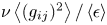$\nu \left \langle (g_{ij})^2 \right \rangle /\left \langle \epsilon \right \rangle$ vs $y^+$ for (a) $(i,j)=(1,2)$, (b) $(i,j)=(2,1)$, (c) $(i,j)=(2,3)$, (d) $(i,j)=(3,2)$, (e) $(i,j)=(3,1)$, (f) $(i,j)=(1,3)$. Thin solid straight lines show $\nu \left \langle (g_{ij})^2 \right \rangle /\left \langle \epsilon \right \rangle =2/15$. The meaning of thick lines is the same as in figure 3.

Figure 7.

Same as in figure 6, but for $|\nu \left \langle (g_{ij})^2 \right \rangle /\left \langle \epsilon \right \rangle -2/15|$. Thin solid straight lines show the slope $-1/2$. The meaning of thick lines is the same as in figure 3; (a) $(i,j)=(1,2)$, (b) $(i,j)=(2,1)$, (c) $(i,j)=(2,3)$, (d) $(i,j)=(3,2)$, (e) $(i,j)=(3,1)$, (f) $(i,j)=(1,3)$.

Let $\lambda _{ijk}$ be the length scale (Taylor microlength scale) defined by

(3.2)\begin{equation} \frac{1}{(\lambda_{ijk})^2} \left\langle u_i({{\boldsymbol{x}}})u_j({{\boldsymbol{x}}}) \right\rangle = \left.-\frac{\partial ^2}{\partial r_k^2} \left\langle u_i({{\boldsymbol{x}}})u_j({{\boldsymbol{x}}+{{\boldsymbol{r}}}}) \right\rangle \right|_{{{\boldsymbol{r}}}=0}. \end{equation}

These length scales are a generalisation of those studied by Vreman & Kuerten (Reference Vreman and Kuerten2014) who computed $\lambda _i\equiv \lambda _{iii}$ in DNS with $Re_\tau$ up to $590$. In TCF, in which the statistics of the fluctuating field ${\boldsymbol {u}}$ are homogeneous in the $x_1$ and $x_3$ directions, we have

(3.3)\begin{equation} \left.-\frac{\partial ^2}{\partial r_k^2} \left\langle u_i({{\boldsymbol{x}}})u_j({{\boldsymbol{x}}}+{{\boldsymbol{r}}}) \right\rangle \right|_{{{\boldsymbol{r}}}={0}} ={-}\delta_{k2} \frac{\partial }{\partial x_2} \left\langle u_i({{\boldsymbol{x}}})\frac{\partial }{\partial x_2} u_j({{\boldsymbol{x}}}) \right\rangle +C_{ikjk}({{\boldsymbol{x}}}). \end{equation}

If the inhomogeneity in the $x_2$ direction is weak so that the first term on the right-hand side of (3.3) and the $x_2$-dependence of $\left \langle u_i({{\boldsymbol {x}}})u_j({{\boldsymbol {x}}}) \right \rangle$ are negligible, then (3.2) and (3.3) with (2.41) and (2.44), (2.45) yield $\lambda _{iik} \propto (y^+)^{1/2}$. This is consistent with the results by Morishita et al. (Reference Morishita, Ishihara and Kaneda2019), who computed $\lambda _{iik}$ (in the present notation) in DNSs of TCF with $Re_\tau$ up to $\approx 5200$.

Figure 8 displays the moments $(\left \langle \epsilon \right \rangle /\nu ) \left \langle g_{1j}g_{2j} \right \rangle =(\left \langle \epsilon \right \rangle /\nu ) \left \langle g_{2j}g_{1j} \right \rangle$. In view of the geometrical symmetry of TCF, it is natural to assume that $\left \langle u_3(x,y,z))u_k(x+x',y+ y',z) \right \rangle =0$ and $\left \langle u_3(x,y,z))u_k(x,y,z+z') \right \rangle =0$ is odd in $z'$ for any $x,y,z$ and $(x',y')$ if $k=1$ or $2$, so that $\left \langle g_{ij}g_{kj} \right \rangle =0$ unless $(i,k)=(1,2)$ or $(2,1)$. Therefore, these moments are not shown here unless $(i,k)=(1,2)$ or $(2,1)$. It is observed that the slope of $(\left \langle \epsilon \right \rangle /\nu ) \left \langle g_{13}g_{23} \right \rangle$ is approximately $-1/2$ in an appropriate range of $y^+$ (e.g. $y^+ \sim 10^3$) in the run with $Re_\tau \approx 8000$, in accordance with (2.46). The difference of the slopes from (2.46) for $j=1$ and $2$ is presumably due to the smallness of the anisotropy correction coefficient $C_{1,1j2j}$ for $j=1$ and $2$.

Figure 8.

Value of $\nu \left \langle (g_{ij}g_{kj}) \right \rangle /\left \langle \epsilon \right \rangle$ vs $y^+$ for $(i,k)=(1,2)$ and $j=1,2,3$; (a) $j =1$, (b) $j = 2$ and (c) $j=3$. Thin solid straight lines show the slope $-1/2$. The meaning of thick lines is the same as in figure 3.

Figure 9 presents the ratios $\left \langle (g_{ij})^2\right \rangle /\left \langle (g_{ii})^2\right \rangle$ for $i,j=1,2$, and $3$ with $i\ne j$. It is observed that, with an increase in $y^+$ i.e. with a decrease in $\gamma$, they approach the isotropy value of two, in accordance with the theoretical conjecture (2.47). The results in figure 9 are consistent with those in Pumir et al. (Reference Pumir, Xu and Siggia2016) who computed the ratios $\xi _i\equiv \left \langle (\partial u_1/\partial x_i)^2\right \rangle /\left \langle (\partial u_1/\partial x_1)^2\right \rangle$ in the DNS of TCF at $Re_\tau \approx 1000$ and showed that the ratios $\xi _2$ and $\xi _3$ decrease towards two near the centre of the channel in the DNS.

Figure 9.

Ratios $\left \langle (g_{ij})^2\right \rangle /\left \langle (g_{ii})^2\right \rangle$ vs $y^+$ for $i, j=1,2$ and $3$ with $i\ne j$; (a) $(i,j)=(1,2)$, (b) $(i,j)=(1,3)$, (c) $(i,j)=(2,1)$, (d) $(i,j)=(2,3)$, (e) $(i,j)=(3,1)$, (f) $(i,j)=(3,2)$. Thin solid straight lines show $\left \langle (g_{ij})^2\right \rangle /\left \langle (g_{ii})^2\right \rangle =2$. The meaning of thick lines is the same as in figure 3.

Figure 10 displays the anisotropy corrections $| \left \langle (g_{ij})^2\right \rangle /\left \langle (g_{ii})^2\right \rangle -2 |$ for $i,j=1,2$ and $3$ with $i\ne j$. The slopes at large $y^+$ are close to $-1/2$ in accordance with (2.47), except for $(i,j)=(2,3)$. The difference in the slope from (2.47) for $(i,j)=(2,3)$ is presumably due to the smallness of the anisotropy correction coefficient $C_{1,12323}$, as suggested by the curve for $(i,j)=(2,3)$ in figure 7(c) and the fast approach to $2$ in the curve for $(i,j)=(2,3)$ in figure 9(d).

Figure 10.

Same as figure 9, but for $| \left \langle (g_{ij})^2\right \rangle /\left \langle g_{ii})^2 \right \rangle -2 |$. Thin solid straight lines show the slope $-1/2$. The meaning of thick lines is the same as in figure 3; (a) $(i,j)=(1,2)$, (b) $(i,j)=(1,3)$, (c) $(i,j)=(2,1)$, (d) $(i,j)=(2,3)$, (e) $(i,j)=(3,1)$, (f) $(i,j)=(3,2)$.

3.4. Energy dissipation rate tensor

Figure 11(a,b,c) presents $\epsilon _{ii}/(2\left \langle \epsilon \right \rangle )$ for $i=1,2$ and $3$. Additionally, figure 12 shows the magnitude of the deviatoric parts $d_{ij}$ of $\epsilon _{ij}/(2\left \langle \epsilon \right \rangle )$ for $\{i,j\}=\{1,2,3\}$, where

(3.4)\begin{equation} d_{ij}\equiv \frac{\epsilon_{ij}}{2\left\langle \epsilon \right\rangle }-\frac{1}{3} \delta_{ij}. \end{equation}

As noted above, a consideration of the geometrical symmetry of TCF gives $\left \langle g_{ik}g_{ik} \right \rangle =0$, so that $d_{ij}=0$ if $(i,j)=(2,3),(3,2), (3,1)$ or $(1,3)$. Therefore, $d_{23}, d_{32}, d_{13}$ and $d_{31}$ are not plotted in figure 12.

Figure 11(a,b,c) demonstrates that $\epsilon _{ii}/(2\left \langle \epsilon \right \rangle )$ for $i=1,2$ and $3$ approach the isotropy value of $1/3$ with an increase in $y^+$ in accordance with (2.48). The slopes of $d_{11}$ and $d_{22}$ from the DNS at $y^+ \sim 10^3$ are approximately $-1/2$ in accordance with (2.48). Regarding $d_{33}$ in figure 12(c), the departure of the slope from $-1/2$ is presumably due to the smallness of $C_{1,3\alpha 3\alpha }$.

Figure 11.

Values of $\epsilon _{ii}/(2\left \langle \epsilon \right \rangle$) for $i=1,2$ and $3$ vs $y^+$. Thin solid straight lines show $\epsilon _{ii}/(2\left \langle \epsilon \right \rangle )=1/3$. The meaning of thick lines is the same as in figure 3.

Figure 12.

Values of $|d_{11}|$, $|d_{22}|$, $|d_{33}|$ and $|d_{12}|=|d_{21}|$. Thin solid straight lines show the slope $-1/2$. The meaning of thick lines is the same as in figure 3.

Using the data of a series of DNSs of TCF with $Re_\tau$ up to $5200$, Lee & Moser (Reference Lee and Moser2019) computed the second invariant $II_\epsilon$ of $d_{ij}$ as suggested by Antonia et al. (Reference Antonia, Kim and Browne1991) and Antonia, Djenidi & Spalart (Reference Antonia, Djenidi and Spalart1994), which is given in the present notation as

(3.5)\begin{equation} II_\epsilon \equiv \tfrac{1}{2} d_{\alpha\beta}d_{\beta\alpha} = \tfrac{1}{2} \left[ (d_{11})^2 + (d_{22})^2+ (d_{33})^2 +2 (d_{12})^2 \right]. \end{equation}

They noted that, in the overlap region ($y^+ \approx 100$ to $y/\delta \approx 0.2)$, $II_\epsilon$ varies as $(y^+)^{-5/4}$, where $2\delta$ is the channel width. This exponent $-5/4$ appears to be consistent with figure 13(a).

In contrast, (2.39), (2.48), (3.4) and (3.5) give

(3.6)\begin{equation} II_\epsilon \approx C_{II} \gamma^2, \end{equation}

and $II_\epsilon \propto (y^+)^{-1}$ for large $y^+$, where $C_{II}$ is a dimensionless constant determined using the constants $C_{1,ijkj}$. Thus, the slope obtained by (2.48) appears to be in conflict with that obtained by DNS. However, it is to be recalled that (2.39) is based on (2.27), which discards possible corrections of the $O(\gamma )$ terms for small $\gamma$ to $\Delta \left \langle g_{ij}g_{mn}\cdots \right \rangle$, as well as corrections due to effects other than the mean shear, which are not taken into account by the parameter $\gamma$.

As regards the correction, say $\Delta _{2\gamma }$, to $\Delta \left \langle g_{ij}g_{mn} \right \rangle$ by terms of $O(\gamma )$, a naive idea suggests that one may approximate it by a term such as $c_2 \gamma ^\alpha$, where $c_2$ and $\alpha (>1)$ are constants. If one simply puts $\alpha =2$, then the addition of the correction term $c_2 \gamma ^2$ to (2.27) gives

(3.7)\begin{equation} II_\epsilon \approx C_{II} {\gamma^2} + D_{II} \gamma^3 . \end{equation}

Substitution of (2.42) into (3.7) gives

(3.8)\begin{equation} {II_\epsilon} \approx C_{II} (y^+)^{{-}1} + D'_{II} (y^+)^{-\beta} , \quad (\beta=3/2), \end{equation}

where $C_{II}, D_{II}$ and $D'_{II}$ are dimensionless constants, and $D'_{II}=CD_{II}$. Here, terms of $O(\gamma ^3)$ in (3.7) and $O((y^+)^{-\beta })$ in (3.8) are ignored.

Regarding possible corrections by effects other than the mean shear, one can consider those related to the finiteness of the distance, say $y$, from the wall. In this respect, it is of interest to note that (2.43) gives $\eta /y \propto (y^+)^{-3/4}$ in the inertial sublayer. If one assumes (i) that such a correction, say $\Delta _w$, due to the finiteness of $1/y$ is linear in $1/y$, so that it is given by the form $\Delta _w \approx c'_w/y$ as a first approximation, and (ii) that the coefficient $c'_w$ depends only on $\nu$ and $\left \langle \epsilon \right \rangle$, then one has $c_w' \propto \eta$, so that $\Delta _w\approx c_w(y^+)^{-3/4}$, where $c_w$ is a dimensionless constant. The addition of such correction term to (2.27) gives ${II_\epsilon }$ but with $\beta =5/4$.

It is of interest to ask how much the difference between the theory and DNS is attributable to these corrections. Figures 13 and 14 may give an idea on this question. Figure 13(b) shows $II_\epsilon /\gamma ^2$ vs $\gamma$. A least squares fit of $II_\epsilon /\gamma ^2$ given by (3.7) with $\beta =3/2$ to the DNS data in the range of $\gamma$ that corresponds to the range $y^+ \in [232,1600]$ provides

(3.9a,b)\begin{equation} C_{II}= 4.40\times 10^{{-}2} , \quad D_{II} = 1.08. \end{equation}

The value given by (3.7) with (3.9a,b) is plotted together with the DNS data. It is observed that $II_\epsilon$ is well approximated by (3.7) in a certain range of $\gamma$.

Figure 14(a) shows ${II_\epsilon }{y^+}$ vs $y^+$. A least squares fit of $II_\epsilon y^+$ given by (3.8) with $\beta =3/2$ and $5/4$ to the DNS data in the range of $y^+ \in [2.6Re_\tau ^{1/2}, 0.2Re_\tau ]\approx [232,1600]$ gives

(3.10a,b)\begin{gather} \beta = 3/2; C_{II}=1.64\times 10^{{-}1}, \quad D'_{II}=4.83, \end{gather}

(3.11a,b)\begin{gather} \beta = 5/4; C_{II}={-}3.16\times 10^{{-}2}, \quad D'_{II}=1.96. \end{gather}

Figure 13.

(a) Second invariant $II_\epsilon$ of tensor $(d_{ij})$. Thin solid straight and dotted straight lines denote the slopes $-1$ and $-5/4$, respectively. (b) Value of $II_\epsilon /\gamma ^2$ vs $\gamma$; broken lines represent the fit (3.7) with $C_{II}=4.40 \times 10^{-2}$ and $D_{II}=1.08$. The meaning of thick lines is the same as in figure 3.

Figure 14.

(a) Value of $II_\epsilon y^+$ vs $y^+$. Broken line shows the fit (3.8) with $\beta = 3/2$, $C_{II}=1.64 \times 10^{-1}$ and $D'_{II}=4.83$, and the dotted line displays the fit (3.8) with $\beta = 5/4$, $C_{II}=-3.16 \times 10^{-2}$ and $D'_{II}=1,96$, and (b) $II_\epsilon$ vs $\gamma$.

The values given by (3.8) with (3.10a,b) and (3.11a,b) are plotted in figure 14(a) together with the DNS data. It is observed that $II_\epsilon y^+$ is well approximated by (3.8) in the range of $y^+ \in [232,1600]$. This result suggests that the difference between the slope $-5/4$ observed in DNS data and $-1$ by the theory is attributable at least partly to the finiteness of $\gamma$. However, the possibility that the slope $-5/4$ is an intrinsic feature and remains constant $-5/4$ in an appropriate range of $y^+$ at $Re_\tau \to \infty$ is not excluded, and the question of how to fix the best value of the exponent $\beta$ in (3.8) is not yet settled.

Figure 13(a) shows that, at small $\gamma$, (e.g. $\gamma < 0.03$), DNS data for $II_\epsilon /\gamma ^2$ do not fit well to (3.6), but blow up like $\propto \gamma ^{m}$ with $m \approx -2$. This result implies that $II_\epsilon \approx$ constant, in the small$-\gamma$ range, as confirmed by figure 14(b), which shows $II_\epsilon$ vs $\gamma$. This disagreement of DNS data with (3.6) is not surprising because the anisotropy in $\epsilon _{ij}$ can in general be induced not only by the mean shear, but also by other factors, in particular the anisotropy of energy-containing eddies, while the effect of the latter is assumed to be negligible compared with those of the former in the derivation of (3.6). In the central region of the channel, the statistics of the large-scale eddies are anisotropic, and their influence on small-scale statistics can remain finite, even if $\gamma$ is very small. This implies that, in this region, the anisotropy measure $II_\epsilon$ can remain finite, independently of the smallness of $\gamma$. This picture is consistent with figure 14(b), which shows that $II_\epsilon$ is small but finite at $\gamma \ll 1$.