1. Introduction
A shock train is a common and complex flow phenomenon in a scramjet isolator, functioning to compress the flow to the required combustion pressure and prevent downstream disturbances from propagating upstream (Matsuo, Miyazato & Kim Reference Matsuo, Miyazato and Kim1999; Gnani, Zare-Behtash & Kontis Reference Gnani, Zare-Behtash and Kontis2016; Huang et al. Reference Huang2023). The main structure of this phenomenon consists of a sequence of shock waves. As the incoming Mach number increases, the shock-wave structure evolves from a
 $\lambda$
-type to an
 $X$
-type (Tamaki et al. Reference Tamaki, Tomita and Yamane1970, Reference Tamaki, Tomita and Yamane1971). The flow structure characterised by
 $\lambda$
-type shock waves is referred to as a normal shock train, while the primary flow structure featuring
 $X$
-type shock waves is known as an oblique shock train (Hunt & Gamba Reference Hunt and Gamba2018).
The primary focus for shock trains lies in their static pressure distributions and dynamic characteristics. In terms of static pressure distributions (Tu & Segal Reference Tu and Segal2010), the initial stage of a normal shock train exhibits a rapid increase in pressure, followed by a more gradual change. For oblique shock trains, the pressure rise exhibits a relatively gradual change, and the slope of the pressure rise remains fairly constant for most of the shock train’s length. According to the empirical relationship proposed by Waltrup & Billig (Reference Waltrup and Billig1973), the pressure rise has a quadratic correlation with the flow direction position, which aligns better with the variations in pressure rise observed in normal shock trains. Consequently, some studies (Merkli Reference Merkli1999; Fotia & Driscoll Reference Fotia and Driscoll2012) that utilised this relationship to predict the pressure rise of oblique shock trains have yielded inaccurate predictions. To address this, Smart (Reference Smart2015) has established a one-dimensional analysis model for accurately calculating the shock train. This model effectively estimates the length of oblique shock trains and provides precise static pressure distribution. The dynamic characteristics of shock trains, also known as self-excited oscillation characteristics under steady backpressure, involve not only the frequency distribution but also the sources that induce this instability. Both normal and oblique shock trains exhibit wideband spectral characteristics (Xiong et al. Reference Xiong, Wang, Fan and Wang2017; James, Vignesh & Kim Reference James, Vignesh Ram and Kim2023). Recent research (Hunt & Gamba Reference Hunt and Gamba2019) on normal shock trains indicates that instability is primarily caused by three sources of disturbances: acoustic waves generated by separation bubble instabilities near the second shock, vortices generated by shear-layer instabilities in separation bubbles that propagate downstream and acoustic waves originating from downstream. However, the instability between the top and bottom walls of oblique shock trains differs due to their asymmetric structure (Xiong et al. Reference Xiong, Wang, Fan and Wang2017). A similar discussion on the sources of disturbances causing instabilities in oblique shock trains is currently lacking.
Since the isolator’s downstream section is directly connected to the combustor, pressure fluctuations from combustion instability significantly affect the shock train (Lin et al. Reference Lin, Jackson, Behdadnia, Jackson, Ma and Yang2022; Laurence et al. Reference Laurence, Karl, Schramm and Hannemann2013). Under these conditions, the shock train undergoes forced oscillations. This phenomenon has attracted significant research attention, leading to various studies (Klomparens, Driscoll & Gamba Reference Klomparens, Driscoll and Gamba2016; Su, Ji & Chen Reference Su, Ji and Chen2016; Gnani et al. Reference Gnani, Zare-Behtash, White and Kontis2018), where downstream excitation is often simplified as periodic disturbances. Given the continuous motion of the shock train, researchers primarily focus on instantaneous static pressure distributions (Edelman et al. Reference Edelman, Gamba, Hunt, Auslender, Donbar and Hagenmaier2021), frequency characteristics (Xiong et al. Reference Xiong, Fan, Wang and Tao2018), disturbance propagation characteristics (Wang, Xiong & Fan Reference Wang, Xiong and Fan2021) and the prediction of shock-motion amplitude (Xiong et al. Reference Xiong, Fan, Wang and Tao2018; Cheng, Wang & Cheng Reference Cheng, Wang and Cheng2019).
Edelman et al. (Reference Edelman, Gamba, Hunt, Auslender, Donbar and Hagenmaier2021) conducted an integrated isolator/combustor test and observed a downstream pressure excitation at 270 Hz, causing the leading shock velocity reaching up to 20 % of the incoming flow velocity. This results in significant changes to the shock-train strength, necessitating a revision in the prediction of its static pressure distribution. This study demonstrates that the prediction model utilising the relative Mach number exhibits better agreement with experimental results compared with the model employing only the incoming Mach number. Xiong et al. (Reference Xiong, Fan, Wang and Tao2018) induced oscillating backpressure by positioning a rotating fan downstream of the isolator. Experimental results demonstrate that as the normal shock train moves upstream, its relative Mach number increases, leading to a greater final pressure rise. Conversely, when the shock train moves downstream, both the relative Mach number of the shock train and final pressure rise decrease. Although the empirical relationship proposed by Waltrup & Billig (Reference Waltrup and Billig1973), adjusted for relative Mach number, could partially predict this trend of change, discrepancies remain between predicted and observed values. In fact, the significance of relative Mach number in moving shock–boundary layer interference has been noted in previous forced oscillation experiments of normal shock waves (Bruce & Babinsky Reference Bruce and Babinsky2008).
To investigate the impact of downstream forced disturbances on shock trains with broadband frequency characteristics, Gillespie & Sandham (Reference Gillespie and Sandham2022) conducted a direct numerical simulation study on forced oscillating normal shock trains within a frequency range of 2.5–40 kHz. They found that high excitation frequencies downstream had minimal effect on the shock train, with high-frequency information dissipating rapidly over a short distance. Conversely, low-frequency backpressure excitation significantly amplified shock-train movement and enhanced self-excited oscillations. In contrast, Xiong et al. (Reference Xiong, Fan, Wang and Tao2018) observed that a downstream excitation frequency of 90 Hz effectively suppressed self-excited oscillations in forced oscillations of oblique shock trains, contradicting the findings from normal shock trains. The disparity in results may be attributed to differences in dynamic characteristics between normal and oblique shock trains, as well as variations in the applied excitation frequencies downstream. Additionally, the asymmetric structure of oblique shock trains leads to disparities in the dynamic characteristics between the top and bottom walls. Further research is necessary to comprehensively understand the effects of forced disturbances on different types of shock trains.
Regarding the propagation characteristics of shock trains under forced oscillation conditions, Edelman & Gamba (Reference Edelman and Gamba2019) conducted an experimental research using Mach 2 and observed that downstream disturbances propagated upstream at a speed closely resembling that of acoustic waves. The propagation speed is found to be dependent on the rate of change of downstream disturbances rather than the specific disturbance amplitude. The study conducted by Wang et al. (Reference Wang, Xiong and Fan2021) demonstrates that the propagation speed of disturbance in a forced oscillating oblique shock train is higher compared with that in a forced oscillating normal shock train, and it remains unaffected by the downstream backpressure. Nevertheless, existing research lacks a comparison with the propagation characteristics of self-excited oscillation disturbances, as well as an analysis of the disparities in disturbance propagation on the top and bottom walls of oblique shock trains.
The rapid prediction of motion amplitude for forced oscillating shock trains is of great practical value, as it can not only determine the operating state of an inlet, but also be used as a part of a control system to prevent inlet unstart. Building upon the empirical relationship established by Waltrup & Billig (Reference Waltrup and Billig1973), Xiong et al. (Reference Xiong, Fan, Wang and Tao2018) considered the influence of relative Mach number on pressure rise in a forced oscillating shock train, thereby developing a prediction model for shock-train-motion amplitude utilising small-perturbation theory methods. This theoretical model well describes variations in shock-train-oscillation amplitude with oscillating backpressure and has been validated experimentally. In the study conducted by Cheng et al. (Reference Cheng, Wang and Cheng2019) on forced oscillating oblique shock trains, low-frequency excitations introduced downstream (12–62 Hz) resulted in negligible relative motion between the leading and second shocks. Consequently, simplifying the shock train as a normal shock and employing prediction formulas for forced oscillating normal shock waves are deemed appropriate for analysing an oblique shock train. However, at higher frequencies such as 120 Hz (Wang et al. Reference Wang, Cheng, Cheng and Xue2018), a significant increase in relative motion between the two shocks occurred, resulting in an escalation of prediction errors. This approach oversimplifies the oblique shock train by disregarding its flow structure asymmetry and the complexity of downstream flows, thereby introducing substantial inaccuracies in practical predictions. Li et al. (Reference Li, Chang, Xu, Yu and Bao2021) utilised the methodology proposed by Smart (Reference Smart2015) to establish a low-order dynamic model for normal and oblique shock-train motions. This model effectively predicts the forced oscillation of shock trains with incident shocks; however, it only considers the leading-shock motion on one side while disregarding the leading-shock motion on the other side. Additionally, the model comprises a set of implicit differential equations that are complex to solve, making the quick prediction of oblique shock-train-motion amplitude unfeasible.
Due to the position of the isolator downstream of the inlet and the disparity between the inlet cowl and ramp length, there is an inconsistency in the actual boundary layer on the top side and bottom side at the entrance of the isolator. However, this crucial point is often overlooked in most studies on isolators, where shock trains are analysed assuming equal-thickness boundary layers on both sides. Recognising this issue, our study introduces different lengths for the top and bottom walls to simulate the asymmetry in the incoming flow’s boundary layer at the entrance of the isolator. This article focuses on oblique shock trains, specifically examining variations in static pressure distributions, frequency characteristics and disturbance propagation properties between shock trains under steady backpressure and periodic excitation backpressure. By comprehensively understanding these aspects, we establish a rapid prediction model for forced oscillating shock trains by combining the characteristics of oblique shock trains with small-perturbation theory methods.
2. Experiment methodology
This experiment was conducted in a supersonic wind tunnel of Nanjing University of Aeronautics and Astronautics. The downstream of the wind tunnel is connected to a 300 m
 $^3$
vacuum tank, while the upstream is open to the atmosphere. The nozzle has a 200 mm
 $\times$
200 mm square exit. The operating time of the wind tunnel is longer than 14 s. Upon initiation of wind tunnel operation, the Mach number at the model entrance reaches 2.85.
Figure 1(a) shows the test model, where the cross-section of the isolator is rectangular with a constant area along the duct. The length of the bottom wall in the constant-area section is 267 mm, while that of the top wall is 187 mm. The duct has a height (
 $h$
) of 15 mm and a width (
 $w$
) of 40 mm. The reference point at
 $x$
= 0 mm is established at the leading edge of the bottom wall. To ensure a fully developed turbulent boundary layer on the bottom-wall side, a rough band is positioned 5 mm from the leading edge. Figure 1(b) shows the position of the model relative to the Laval nozzle. This position can avoid the influence of expansion waves generated from the nozzle outlet on the incoming flow of the test model. A movable Pitot tube is used to profile the boundary layer at
 $x$
= 93 mm, yielding a measured thickness of 3.70 mm (at 99 % mainstream velocity). After obtaining the velocity profile of the boundary layer, the Crocco–Busemann formula is employed to derive the temperature and velocity distribution, assuming a turbulence recovery factor
 $r$
= 0.89 and an adiabatic wall condition; then the displacement thickness
 $\delta ^*$
, momentum thickness
 $\theta$
and Reynolds number
 ${\textit{Re}}_\theta$
are obtained. Additionally, the method proposed by Kendall & Koochesfahani (Reference Kendall and Koochesfahani2008) is used to estimate the skin-friction coefficient
 $C_{\!f,0}$
. This estimation approach has been extensively utilised in previous studies (Touré & Schülein Reference Touré and Schülein2020; Li et al. Reference Li, Zhang, Tan, Jin and Li2022), and the parameters for the incoming flow are presented in table 1.
Experimental set-up: (a) diagram of the test model; (b) relative position of the test model and Laval nozzle.

Incoming flow parameters.

The expansion section is positioned downstream of the isolator. To accommodate the disturbance block which is marked by orange in figure 1, a constant-area section with a height (
 $h_1$
) of 28 mm is incorporated within the expansion section. A disturbance block, with an elliptical cross-section, is installed upstream of the throttling cone. For the state discussed below, the minor axis (a) of the ellipse is fixed at 0.35
 $w$
, the major axis (b) is set to 0.80
 $w$
and the height (
 $h_2$
) of the disturbance block corresponds to 0.5
 $h_1$
. Subsequent sections investigate various pressure disturbance amplitudes by maintaining a constant minor axis and adjusting either the elliptical height or major axis accordingly. The specific dimensions are introduced in detail below. The disturbance block is connected to a model aircraft motor, with its vertical centre aligned with the centre of the top and bottom walls of the duct. Periodic disturbances are generated within the duct by rotating the disturbance block. A throttling cone is positioned at the end of the expansion section, creating a downstream throttling throat upon movement, subsequently leading to shock-train formation in the isolator. The average position of the shock train can be adjusted by varying the position of the throttling cone. For steady shock-train tests, the disturbance block is removed, leaving only the downstream throttling system. During forced oscillation shock-train tests, these two systems collaborate to achieve periodic excitation.
To acquire the dynamic characteristics of the shock train, 11 dynamic pressure transducers were installed on both the top and bottom walls of the model, with identical
 $x$
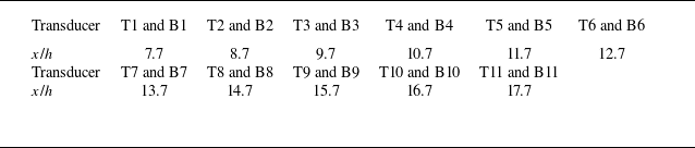
coordinates on both sides. The specific locations for displacement transducers are provided in table 2. Transducers placed on the top wall are denoted as T, while those on the bottom wall are denoted as B. The distance between adjacent transducers along the
 $x$
direction is consistently set at 1.0
 $h$
. The dynamic pressure transducer used in this experiment was a CYG-503AS, manufactured by Double Bridge Inc., with a measurement range of 100 kPa and a sampling frequency of 20 kHz. A ’Z-type’ schlieren system was employed to observe the shock train, with figure 1 showing the placement of the optical glass within the model. The high-speed camera used was an NAC Memrecam HX-3, equipped with a Nikon AF vr80–400 mm
 $f$
/4.5–5.6d optical lens. The acquired schlieren images possessed a resolution of 1664
 $\times$
256 (7 pixels mm
 $^{-1}$
) and were captured at a sampling rate of 6000 frames per second and an exposure time of 50 μs.
Transducer location details.

(a–c) Schematic image of shock-train structure and leading-shock identification under steady backpressure.

3. Experimental results
3.1. Shock-train behaviours under steady backpressure
Before conducting research on a forced oscillating shock train, the behaviours of oblique shock trains under steady backpressure are investigated. Figure 2 illustrates a typical instantaneous schlieren image of the shock train. When the incoming Mach number is 2.85, an
 $X$
-type structure is observed in the leading shock within the duct. Due to differing thicknesses of the boundary layers on the bottom and top walls at identical
 $x$
positions (figure 2
a), the bottom wall experiences greater separation, resulting in a tilt towards the top wall in the mainstream flow of the shock train.
To determine the leading-shock position, this study initially converts the greyscale image (figure 2
b) into a binary image (figure 2
c). Noise in the flow field is then eliminated by assigning a value of 1 (white) to the centre pixel if the sum of its neighbouring values exceeds a certain threshold; otherwise, it is assigned a value of 0 (black), resulting in figure 2(c). The position of the bottom leading shock is detected by sequentially scanning from left to right and bottom to top. Similarly, scanning from left to right and top to bottom identifies the top leading shock. The positions of these shocks are indicated by red markers in figure 2(c). By correlating pixel points with geometric positions, the precise physical location of the leading shock is determined. Finally, manual adjustments are made to identify any implausible positions. The primary source of error in this methodology lies in selecting an appropriate threshold for converting greyscale images to binary images. The maximum potential error from this threshold selection is directly related to the thickness of the leading shock (Hunt & Gamba Reference Hunt and Gamba2019). In our study, we observed a maximum thickness of approximately 2 mm for the leading shock, leading to a potential positional error range of (
 $-$
2, 2 mm) in determining the position of the leading shock.
The instability of oblique shock trains under steady backpressure has been extensively studied. Figure 3 illustrates pressure variations recorded by transducers T11 and B11 under steady-backpressure conditions. Notably, a significant irregular fluctuation in the pressure curve is observed, with greater amplitude on the top wall compared with the bottom wall. These findings indicate pronounced self-excited oscillation characteristics of the shock train.
After obtaining the power spectrum density (PSD) distributions for each pressure transducer, linear interpolation on the PSD data between adjacent transducers is performed to generate figures 3(b) and 3(c). Additionally, these figures indicate the positions of both most upstream (
 $U$
) and most downstream (
 $D$
) leading shocks. Here T and B represent the top and bottom, respectively, and
 $U_{{T}}$
denotes the most upstream position of the leading shock on the top wall. Other abbreviations follow similar connotations. Figure 4 shows the corresponding schlieren images. Due to the inclination of the shock train’s core flow towards the top wall, both the leading and downstream shocks exhibit oscillations, corresponding to significant pressure fluctuations. Consequently, for the top wall, higher PSD values are observed not only near the leading shock but also downstream. For the bottom wall, except for the leading shock, which exhibits continuous oscillations and induces significant pressure changes, all transducers located downstream lie within a separation zone where pressure fluctuations are insignificant, resulting in low PSD values.
(a) Static pressure histories at the downstream transducer under steady backpressure. The PSD distributions along the transducers: (b) the top-wall side; (c) the bottom-wall side.

Schlieren images: (a) upstream leading shocks; (b) downstream leading shocks.

3.2. Shock-train behaviours under periodic excitation backpressure
Periodic excitations applied downstream induce periodic oscillations in the shock train. Figure 5 presents schlieren images capturing the shock train at various positions within one cycle at a downstream excitation frequency of 199.5 Hz. The frequency selected is close to the downstream frequency measured in a scramjet test (Jiang et al. Reference Jiang, Zhang, Liu, Wang and Luo2021). Throughout this motion, the shock train’s core flow consistently inclines towards the top wall. The most notable differences in the leading-shock structure occur at
 $t_1$
= 1.50 ms and
 $t_1$
= 4.17 ms, where the x positions of the leading shock are relatively close but moving in the opposite direction. The velocity of the leading shock is determined by the schlieren snapshot. When moving upstream (
 $t_1$
= 1.50 ms), the moving Mach number of the leading shock is approximately 0.23, whereas when moving downstream (
 $t_1$
= 4.17 ms), it increases to around 0.27. Compared with moving upstream, the leading-shock structure weakens significantly when moving downstream. This phenomenon also occurs during the motion of a normal shock train (Yu et al. Reference Yu, Tan, Li, Li, Zhang and Wang2023), where the weakening of the leading shock indicates a significant change in the instantaneous static pressure distribution of the shock train. In addition, the leading-shock angle does not change significantly during the movement of the shock train. Yu et al. (Reference Yu, Tan, Li, Li, Zhang and Wang2023) also discovered a similar phenomenon and provided an explanation for it.
Instantaneous flow structures of shock train at different times within a typical cycle under downstream periodic excitation.

The instantaneous static pressure distribution at each moment in figure 5 and the average pressure distribution under steady backpressure are presented in figure 6. Significant pressure fluctuations are observed along the top wall, whereas the pressure curve on the bottom wall consistently trends upward. These differences arise from the varying boundary-layer thicknesses on each wall and the differential buffering effects on the expansion waves generated by separation bubbles. Additionally, the linear characteristic of the bottom wall’s pressure distribution becomes more pronounced with increasing Mach number, contrasting with the clear quadratic characteristic observed in normal shock trains (Merkli Reference Merkli1999; Huang et al. Reference Huang, Tan, Sun and Wang2018; Yuan et al. Reference Yuan, Zhang, Liao, Wan, Liu and Lu2024). Notably, both the schlieren image of the shock train in figure 5 and the pressure distribution in figure 6 reveal that the shock train is not fully developed. In the schlieren image, shock waves are still visible near the duct outlet at
 $t_1$
= 3.33 ms (the longest shock train), and significant pressure fluctuations along the top wall at this moment suggest that the shock train has not yet reached the mixing region. This observation is attributed to the length of isolator (
 $\approx$
10
 $h$
) used in the current study. It is worth noting that this isolator length approximates those employed in practical engineering applications (Tan, Sun & Huang Reference Tan, Sun and Huang2012), aligning our research results more closely with an actual situation. Comparing the static pressure distribution of the shock train at
 $t_1$
= 1.50 ms and
 $t_1$
= 4.17 ms on the bottom wall reveals that as the shock train moves upstream, the maximum pressure rise increases, while downstream movement results in a decrease. This phenomenon indicates that the shock train adjusts its relative Mach number to match downstream pressure changes. Due to the shock train’s nearly identical length at both moments, its average pressure rise slope undergoes significant changes during its motion.
Average pressure distributions of different walls under steady backpressure and instantaneous pressure distributions of these walls under periodic excitation backpressure: (a) the top-wall side; (b) the bottom-wall side.

In addition, it is worth mentioning that background shock waves appear in figure 5. Despite efforts to align the model consistently with the incoming flow direction, factors such as the leading-edge chamfer, viscosity and other influences make it nearly impossible to eliminate these background shock waves. However, as observed in figures 5 and 6, the background shock waves do not have a significant impact on the shock-train structure and pressure distribution, so these are weak background shock waves.
Firstly, the static pressure distribution of the bottom wall is evaluated using the Waltrup–Billig empirical relationship (Waltrup & Billig Reference Waltrup and Billig1973; Sullins Reference Sullins1992), where
 $k_{wb}=50(\sqrt {\theta h}/Re_\theta ^{0.2})$
and
 $x_l$
is the distance from the beginning of the pressure rise point. As shown in figure 7(a), after translating the pressure rise curve, both the most upstream and downstream instantaneous pressure distributions during the motion and the average pressure distributions under different steady backpressures deviate from the empirical relationship, so a new method is needed to evaluate the pressure rise change. The average pressure rise slope of the shock train in this study is determined through least-squares fitting of the pressure rise curve. The selected pressure transducers include the last undisturbed transducer as well as other disturbed transducers. In figure 6, the red dashed line represents the least-squares fitting curve for the average pressure rise of the steady shock train, with similar fitting applied to other pressure rise curves. For example, when
 $t_1$
= 0 ms, the fitting transducers selected are B7–B11, and the same principle is followed at other moments. It is evident that the average pressure rise slope exhibits periodic variations during the motion of the shock train. Figure 7(b) illustrates that at the most downstream position of the shock train, the average slope of pressure rise closely approximates that observed under steady backpressure, whereas at the most upstream position, it decreases. This phenomenon occurs due to the gradual flattening of the pressure rise curve as the shock train lengthens, leading to a decrease in its average slope. As the shock train moves upstream, its relative Mach number increases, resulting in an increase in the average pressure rise slope. Conversely, when it moves downstream, both its relative Mach number and average pressure rise slope decrease.
(a) Static pressure distributions of the bottom wall compared with the Waltrup–Billig empirical relationship. (b) Average slope of pressure rise on the bottom wall under steady backpressure and instantaneous pressure rise slope on this wall under periodic excitation backpressure.

When periodic excitation backpressure is applied downstream, as shown in figure 8(a), the pressure exhibits significant periodic fluctuations. High-frequency random fluctuations are more pronounced on the top wall than on the bottom wall. The PSD distribution in figure 8 along each transducer indicates the presence of harmonics in the flow field. Furthermore, the region significantly affected by pressure disturbances corresponds to the area influenced by the shock train’s motion. Notably, the peak PSD values on both the top and bottom walls occur during the shock train’s movement rather than at its most upstream position.
(a) Static pressure histories at the downstream transducers under periodic excitation backpressure. The PSD distributions along the transducers: (b) the top-wall side; (c) the bottom-wall side.

(a) The leading-shock trajectory for 10 cycles. The PSD distributions along the transducers: (b) the top-wall side, with interpolation; (c) the bottom-wall side, with interpolation.

Figure 9(a) shows the leading-shock trajectory for 10 cycles. On the top-wall side,
 $U_{{T}}$
at
 $x/h$
= 12.0 and
 $D_{{T}}$
at
 $x/h$
= 16.7. On the bottom-wall side,
 $U_{{B}}$
at
 $x/h$
= 11.7 and
 $D_{{B}}$
at
 $x/h$
= 17.0. At this time, the accidental motion of the shock train is no longer representative. Therefore, the average of the most upstream and downstream positions of the leading shock with 10 cycles are used. The symbols in figures 9(b) and 9(c) are modified accordingly. To observe the changes in the self-excited oscillation characteristics of the shock train, we set the range of the legends in figures 9(b) and 9(c) to be consistent with figure 3. Additionally, due to the linear interpolation between adjacent transducers, the difference between the identified leading-shock position and actual pressure disturbance position (figure 2
c), using the position where the PSD value vanishes in this figure to determine the most upstream position of the shock train is unreasonable. Similar to the pressure changes observed under steady backpressure, the self-excited oscillation characteristics are more pronounced on the top wall alongside these periodic fluctuations. The PSD distribution indicates that after applying periodic disturbances downstream, higher harmonics are present in the flow field, with this phenomenon being more noticeable on the top wall than on the bottom wall. Furthermore, the PSD distribution reveals that the self-excited oscillation characteristics of the forced oscillating shock train are attenuated compared with those under steady backpressure. In other words, the periodic pressure disturbance downstream weakens the self-excited oscillation characteristics of the shock train, nearly eliminating these features entirely on the bottom-wall side, where only periodic fluctuations remain.
Correlation coefficient and disturbance propagation time between each transducer and the most downstream transducer: (a) under steady backpressure; (b) under periodic excitation backpressure. (c) Static pressure histories of T9, T10 and T11 transducers under periodic excitation backpressure.

3.3. Analysis of disturbance propagation characteristics
To determine the direction of disturbance propagation and the correlation between each measurement point and downstream disturbance, a two-point cross-correlation analysis is conducted with T11 as a reference point. The two-point cross-correlation analysis is a time-domain analysis method. This method is often used to evaluate the time delay between two time series, and its normalised correlation degree can reflect the similarity between two time series. The correlation coefficient is a function of the time delay (Wang et al. Reference Wang, Chang, x. and Yu2020; Jenquin, Johnson & Narayanaswamy Reference Jenquin, Johnson and Narayanaswamy2023). As shown in figure 10, this analysis allows us to obtain the cross-correlation relationship (
 $Co$
(T
 $i$
, T11)) between pressure transducers on the top wall and downstream pressure transducer T11,
 $i$
ranging from 1 to 10. Similarly, using B11 as a reference point, we can establish cross-correlation relationships (
 $Co$
(B
 $i$
, B11)) for pressure transducers on the bottom wall. Additionally, the value of
 $Co$
(
 $\tau$
) at the maximum correlation coefficient and the time delay
 $\tau$
at the peak are statistically analysed. A positive correlation coefficient indicates that pressure fluctuations are in phase with downstream pressure changes, while a positive time delay suggests that disturbances lag behind downstream disturbances (Wang et al. Reference Wang, Chang, x. and Yu2020; Jenquin et al. Reference Jenquin, Johnson and Narayanaswamy2023). Considering the transducer sampling frequency of 20 kHz, the maximum error in calculating time differences between relevant peaks during computation is approximately 0.1 ms.
Firstly, we analyse the propagation of disturbances in the shock train under steady backpressure. In this condition, a strong correlation is observed between T11 and the pressure transducer near the leading shock, whereas other downstream transducers show weaker correlations with T11. Similar characteristics are observed in normal shock trains (Hunt & Gamba Reference Hunt and Gamba2019), where downstream disturbances primarily affect the region near the leading shock. However, there are no significant changes in correlation coefficients between B11 and the bottom-mounted transducers affected by the shock train.
As shown in figure 10(b), when periodic disturbances are introduced downstream, the correlation coefficient between each transducer affected by the shock train and the most downstream transducer increases significantly, regardless of whether it is located on the top or bottom wall. Additionally, within the region influenced by the shock train, the correlation coefficient is consistently higher for the bottom wall compared with the top wall. Specifically, the correlation coefficient for the bottom wall maintains a stable trend, consistently hovering around 0.9. As for the top wall, the highest correlation coefficients are still observed within the range of leading-shock motion.
From the perspective of disturbance propagation time (with a disturbance correlation coefficient greater than 0.2), under steady backpressure, disturbances propagate from upstream to downstream on the bottom wall, while on the top wall, they propagate from downstream to upstream initially. Based on disturbance propagation characteristics observed in normal shock trains (Hunt & Gamba Reference Hunt and Gamba2019), it can be inferred that downstream acoustic disturbances dominate the bottom wall, whereas acoustic waves generated by separation bubble instability (near the second shock) and vortices from the shear layer dominate the top wall, both propagating from upstream to downstream. In forced oscillating shock trains, disturbance propagation times on the top and bottom walls tend to be consistent within the range of leading-shock motion, with downstream disturbances occurring first. This observation indicates that periodic disturbances enhance the propagation of downstream acoustic disturbances.
The pressure signal at T10 exhibits interesting characteristics (figure 10 c), with inconspicuous periodicity in the static pressure history and a low correlation coefficient with T11. Additionally, the direction of disturbance propagation at T10 does not align with that at B10. This discrepancy arises because T10 is always located downstream of the leading shock, where it is influenced by acoustic waves generated by separation bubble instability and vortices induced by the shear layer, disrupting the periodicity of its pressure signal. Conversely, T11 and B11 are close to the downstream expansion section and directly subjected to downstream disturbances. The pressure changes at these positions are highly synchronised, exhibiting clear periodicity. Consequently, the correlation coefficient between T10 and T11 is relatively low, and the disturbance propagation time is uncertain due to the aforementioned factors. However, B10, being within the separation bubble, experiences minimal impact from self-excited oscillations in the shock train, maintaining a high correlation with downstream transducers and exhibiting distinct disturbance propagation characteristics compared with T10.
4. Modelling of unsteady oblique-shock-train motions
4.1. Analytical study
Based on the research discussed above, three key insights have been identified. Firstly, when the shock train is not fully developed at high Mach numbers, the static pressure distribution along the large separation side exhibits linear characteristics. Secondly, applying periodic backpressure downstream causes the shock train to adjust its relative Mach number to match downstream pressure changes, resulting in periodic changes in the average pressure rise slope of the bottom wall. Thirdly, after periodic excitation is applied, there is a strong correlation between the bottom-wall pressure transducers and outlet pressure transducers in the region affected by the shock train. These common characteristics of forced oscillating oblique shock trains are crucial for understanding and modelling their motion amplitudes.
To quickly predict the motion amplitude of the oblique shock train, a simple analysis is conducted below. The primary challenge is accurately characterising the variations in pressure rise within the shock train. Currently, two common methods are used for modelling pressure rise. One method relies on empirical relationships derived from fitting pressure data, such as the Waltrup–Billig quadratic relationship between incoming Mach number and pressure rise (Waltrup & Billig Reference Waltrup and Billig1973). However, this method is inadequate for predicting not fully developed oblique shock trains due to differences in pressure distribution between normal and oblique shock trains (figure 7 a). Another method, proposed by Smart (Reference Smart2015), involves quasi-one-dimensional analysis of shock trains, effectively estimating their length and pressure distribution. However, this model’s implicit differential equations are complex to solve, making rapid prediction of pressure rise distributions unattainable. Nevertheless, the diffuser model proposed by Ortwerth (Reference Ortwerth2001), provides an important relationship, enabling empirical prediction of the inverse pressure gradient within the shock train:
 \begin{equation} \frac {{\rm d}p}{{\rm d}x}=\frac m{D_h}C_{\!f}\left (\frac {\rho u^2}2\right )\!, \end{equation}
where
 $D_h$
is the hydraulic diameter,
 $C_{\!f}$
is the skin-friction coefficient at the initial separation point of the shock train and
 $m$
is an empirical constant determined through experimental data. Initially, Ortwerth (Reference Ortwerth2001) used
 $m$
= 45, but Smart (Reference Smart2015) found that
 $m$
= 50 provides better predictions for fully developed shock trains. However, Li et al. (Reference Li, Chang, Xu, Yu, Bao and Song2017) discovered that to accurately predict their experimental results for not fully developed shock trains, the value of
 $m$
needs to be adjusted to 75 for normal shock trains and 65 for oblique shock trains. Therefore, it can be concluded that if this method is applied to improve predictions for specific working conditions, appropriate corrections should be made to the value of
 $m$
.
When the incoming Mach number is 2.7, Li et al. (Reference Li, Chang, Xu, Yu, Bao and Song2017) employed Smart’s model to comprehensively simulate the pressure rise of an oblique shock train. Analysis of the predicted pressure curve reveals favourable linear characteristics within a range of approximately 6
 $h$
. In other words, this approach allows for an approximate first-order relationship in modelling the initial pressure rise distribution of the shock train. Furthermore, the study of Smart (Reference Smart2015) demonstrates that during this initial stage of pressure rise in the oblique shock train,
 $\rho u^2/2$
can be approximated as being equal to
 $\rho _0 u_0^2/2$
of the incoming flow. Thus, this paper proposes a simplified approach to predict the pressure rise of the shock train based on the above knowledge. By assuming a constant
 $C_{\!f}$
value along the duct and considering that the shock train has not yet achieved complete pressure rise,
 $\rho u^2/2$
is replaced with
 $\rho _0 u_0^2/2$
. The corrected
 $m$
value can then be determined by combining the average pressure rise slope of the large separation side of the steady shock train. Furthermore, by neglecting variations in static pressure along the duct without interference from the shock train, an approximation for the pressure rise distribution of oblique shock trains can be derived using the following formula:
 \begin{equation} p=k_1{u_0}^2x+p_0 ,\end{equation}
where
 $k_1=\rho _0mC_{\!f,0}/2/D_h$
. The proposed formula based on Ortwerth’s pressure rise formula (Ortwerth Reference Ortwerth2001; Smart Reference Smart2015) significantly simplifies the prediction of pressure rise distribution in an oblique shock train which is not fully developed. This approach enables a rapid estimation of pressure rise using incoming flow parameters while accurately capturing the linear characteristics of pressure rise exhibited by the oblique shock train.
Schematic diagram of the motion of an oblique shock train under downstream micro-pressure disturbance.

Average slope of bottom-wall pressure rise under steady backpressures. LMM, linear mixed-effects model.

We analyse the motion of the shock train under downstream micro-pressure disturbance in combination with figure 11. In a steady state, the downstream pressure is
 $\overline {p}_{T}$
, the corresponding length of the shock train is
 $\overline {x}$
, the velocity at the front of this shock train is
 $\overline {u}_{0}$
and the static pressure is
 $\overline {p}_{0}$
.
As shown in figure 12, using the same
 $x_l$
coordinates as in figure 7, the static pressure distributions under different steady backpressures are well overlapped together. The average pressure distribution exhibits linear characteristics. Linear regression applied to each curve yields
 $R^2$
values between 0.912 and 0.977, confirming the linearity of the pressure rise curves at each backpressure. However, since the slopes of individual curves vary and may be biased due to the limited number of transducers, determining an average slope is necessary. To achieve this, linear mixed-effects models are employed (Pinheiro & Bates Reference Pinheiro and Bates1996; West et al. Reference West, Welch and Galeki2022), providing a rigorous analysis of overall trends by accounting for within-group variance, the sample size of each group and the deviation of each group’s slope from the overall slope (between-group variance). Using this approach, the average slope can be determined and we can use the following equation to approximate it:
 \begin{equation} \overline {p}_T=k_1\overline {u}_0^2\overline {x}+\overline {p}_0. \end{equation}
Schematic diagram of pressure distribution change after pressure disturbance is applied downstream.

When a pressure disturbance
 $p_T^{\prime }$
is applied downstream, the position of the oblique shock train changes, and its motion distance is
 ${x}_{s}^{\prime}$
. As illustrated in figure 11, this disturbance reduces the length of the shock train, so
 \begin{equation} { x'=-{x}_{s}^{\prime}}. \end{equation}
The corresponding velocity change is
 ${u}_{s}^{\prime}$
. However, as the shock train moves downstream, the relative velocity decreases from the perspective of the shock train; thus the relative velocity change is
 \begin{equation} { u'=-{u}_{s}^{\prime}} \end{equation}
and the instantaneous dynamic pressure of the shock train is
 $\rho _0(u_0+u')^2/2$
.
After applying the quasi-steady-state assumption which is also applied in the modelling of normal shock waves (Bruce & Babinsky Reference Bruce and Babinsky2008) and shock trains (Xiong et al. Reference Xiong, Fan, Wang and Tao2018) (i.e. during the micro-displacement process, the shock train still satisfies the relationship obtained under steady backpressure), we can derive the following equation:
 \begin{equation} { \overline {p}_T+p_T^{\prime }=k_1(\overline {u}_0+u^{\prime })^2(\overline {x}+x^{\prime })+\overline {p}_0+p^{\prime }}, \end{equation}
where
 $p_T^{\prime }$
represents the downstream pressure change and
 $p^{\prime }$
represents the pressure change in front of the shock train. In the constant-area rectangular duct, the flow gradient of flow parameters caused by the naturally growing boundary layer upstream of the shock train is negligible, and the influence of weak background waves in the duct is minimal. This is evident from the static pressure distribution along the duct without throttling in figure 6. Therefore,
 $p^{\prime }$
is ignored. The same assumption is used in normal shock-train modelling (Xiong et al. Reference Xiong, Fan, Wang and Tao2018):
 \begin{equation} \overline {p}_T+p_T^{\prime }=k_1(\overline {u}_0+u^{\prime })^2(\overline {x}+x^{\prime })+\overline {p}_0. \end{equation}
The pressure distributions described by (4.3) and (4.7) are shown in figure 13. Notably, (4.7) implies that when the downstream disturbance causes the shock train to move downstream, negative velocity fluctuations will occur, leading to a reduction in the average slope of pressure rise. Conversely, an increase in the average slope of pressure rise is observed, which aligns with the phenomenon identified in figure 7. By subtracting (4.3) from the (4.7), the following equation is obtained:
 \begin{equation} {k_{1}\bigl(\overline {x}u^{\prime 2}+2\overline {u}_{0}\mkern 2mu \overline {x}u^{\prime }+\overline {u}_{0}^{2}x^{\prime }+u^{\prime 2}x^{\prime }+2\overline {u}_{0}u^{\prime }x^{\prime }\bigr)=p_{T}^{\prime }} .\end{equation}
There are three nonlinear terms (
 $k_{1}\overline {x}u^{\prime 2}$
,
 $k_{1}u^{\prime 2}x^{\prime }$
,
 $2k_{1}\overline {u}_{0}u^{\prime }x^{\prime }$
) and two linear terms (
 $2k_{1}\overline {u}_{0}\mkern 2mu \overline {x}u^{\prime }$
,
 $k_{1}\overline {u}_{0}^{2}x^{\prime }$
). The presence of nonlinear terms prevents the derivation of a general analytical solution. Therefore, we analyse the proportional relationship between the nonlinear and linear terms. Assuming that
 $x^{\prime }$
approaches 0 while
 $u^{\prime }$
remains finite, the nonlinear terms
 $k_{1}u^{\prime 2}x^{\prime }$
and
 $2k_{1}\overline {u}_{0}u^{\prime }x^{\prime }$
become negligible, leaving the nonlinear term
 $k_{1}\overline {x}u^{\prime 2}$
as the primary focus of analysis. A quantitative evaluation of this term, performed using the regular perturbation method (Hinch Reference Hinch1991) and supported by the experimental results presented later (see Appendix A), shows that it contributes a maximum correction of only about 2 % to the predicted amplitude. Consequently, this term can be neglected to simplify the equation. This treatment is also consistent with previous studies, where similar nonlinear terms were omitted (Xiong et al. Reference Xiong, Fan, Wang and Tao2018). The equation can therefore be simplified as follows:
 \begin{equation} {2k_{1}\overline {u}_{0}\mkern 2mu \overline {x}u^{\prime }+k_{1}\overline {u}_{0}^{2}x^{\prime }=p_{T}^{\prime }}. \end{equation}
From the perspective of shock-train physical behaviour, this omission is also reasonable. As shown in figure 9, the shock-train trajectory approximates a sine curve, and the absence of observable chaotic phenomena indicates that nonlinear effects are not dominant under the current conditions. Equation (4.9) describes the relationship between the displacement of the shock train and downstream pressure disturbance. For downstream oscillating pressure signals, although harmonics contribute to the pressure oscillation (figure 9), it is challenging to accurately obtain the amplitude and phase of each frequency component by decomposing the discrete pressure signal. To simplify the problem and given the weak influence of harmonics on the outlet pressure signal waveform (figure 8), this signal is simplified into a single-frequency sine wave (Xiong et al. Reference Xiong, Fan, Wang and Tao2018). However, the amplitude of the simplified signal is still obtained from the actual pressure signal, and it can be expressed by the following equation:
 \begin{equation} p_T(t)\approx \overline {p}_{T}+A_T\overline {p}_{T}\sin (\omega t+\beta ), \end{equation}
where
 $A_T=\Delta p_T/\overline {p}_T$
,
 $\Delta p_T$
is the oscillation amplitude of the pressure signal, the method for obtaining it will be introduced in next section, and
 $\omega$
is the circular frequency. For a single-frequency downstream excitation, the phase
 $\beta$
of the pressure signal does not affect the oscillation amplitude of the shock train. Therefore, the downstream pressure oscillation can be written as
 $p_T^{\prime }=A_T\overline {p}_T\sin (\omega t)$
, and by substituting it into the (4.9), the following equation can be obtained:
 \begin{equation} \frac {{\rm d}x^{\prime }}{{\rm d}t}+Px^{\prime }=Q\sin (\omega t). \end{equation}
Since we also obtain a linear differential equation, the basic form of the equation is consistent with previous research (Xiong et al. Reference Xiong, Fan, Wang and Tao2018), but there are significant differences in the meanings of the specific coefficients. Here
 \begin{align} P&={\overline {u}_0}/\left (2\overline {x}\right )\!, \end{align}
 \begin{align} Q&=A_T\overline {p}_T/\left (2 k_1{\overline {u}_0}\mkern 2mu \overline {x}\right )\!. \end{align}
Considering the initial condition
 $x^{\prime }(0) = 0$
, the solution of (4.11) is
 \begin{equation} {x^{\prime }(t)=A_1[\sin (\omega t+\psi )]+A_1\frac {{\rm e}^{-Pt}}{\sqrt {P^2/\omega ^2+1}}}. \end{equation}
In this equation,
 $A_1=Q/\sqrt {P^2+\omega ^2}$
and
 $\psi =-\arctan (\omega /P)$
.
The above equation describes the displacement change of the shock train resulting from the application of a sinusoidal backpressure downstream. The first term represents the periodic amplitude change and the second term is the attenuation term. However, this attenuation term decays rapidly and has almost no effect on the periodic amplitude change. The following section provides examples for further explanation.
The modelling process shares some similarities with previous research (Xiong et al. Reference Xiong, Fan, Wang and Tao2018), but due to the asymmetric shock-wave structure and approximately linear pressure rise, the previous model is no longer applicable. Firstly, previous studies did not account for the difference in pressure between the top and bottom walls, which significantly affects prediction accuracy. In addition, the previous model is based on the Waltrup–Billig relationship (Waltrup & Billig Reference Waltrup and Billig1973) for modelling work, while this research is based on Ortwerth’s pressure rise formula (Ortwerth Reference Ortwerth2001). Therefore, there is a significant difference in the final equation obtained.
4.2. Experimental verification
In contrast to normal shock trains in previous work (Xiong et al. Reference Xiong, Fan, Wang and Tao2018), oblique shock trains in the current research feature an asymmetric leading shock. Therefore, separate calculations are necessary to determine the amplitude of motion for each side of the leading shock. Additionally, the non-uniform pressure distribution along the top and bottom walls makes the choice of downstream pressure transducer critical. While modelling primarily emphasises characteristics related to the bottom wall, considering the differences in the transducer positions of the top and bottom walls is the feature of this research. To quantify the error introduced by top-wall information, we analyse how this affects prediction accuracy. Finally, pressure fluctuations near the outlet are evaluated using transducers on both walls and their averaged values. For this purpose, transducers T11 and B11 have been selected.
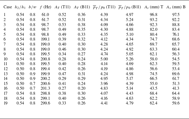
In this experiment, disturbance blocks of varying sizes are used to investigate pressure excitation amplitudes. The minor axis a of these disturbance blocks remained fixed at 0.35
 $w$
, while other dimensions are listed in table 3. The experimental parameters, including pressure oscillation amplitude
 $A_T$
, average pressure
 $\overline {p}_T/p_0$
and shock-train-motion amplitude
 $A_s$
, listed in the table are determined by randomly selecting data from 10 cycles and calculating their averages. Specifically,
 $A_T$
is obtained by calculating the mean value of the difference between the maximum and minimum values across these cycles. Currently, the frequency range of downstream excitation in this experiment is 61.0–299.6 Hz. The error in measuring the leading-shock-motion amplitude on both top and bottom walls is within (
 $-$
4, 4 mm), primarily due to limitations in schlieren image processing techniques.
Statistics of experimental results.

Prediction results of shock-train-motion amplitude using different pressure transducer data: (a) the top-wall side; (b) the bottom-wall side.

By calculating the average slope of pressure rise under steady backpressures in figure 12, a value of
 $m$
can be obtained as 54.3. Combined with the incoming flow parameters,
 $k_1$
can be obtained as 0.334 Pa s
 $^2$
m
 $^{-3}$
, and
 $\overline {u}_0$
is 608 m s−1. Furthermore, statistical results from table 3 indicate minimal disparities in shock-train-motion amplitudes between the top and bottom walls.
Firstly, we evaluate the attention term of the model presented in (4.14). Since this term increases with excitation frequency, the maximum excitation frequency of 299.6 Hz is used for evaluation. With
 $\overline {x}=0.1$
m and after one period (1/299.6 s), the second term can be obtained as
 $2.1\times 10^{-5} A_1$
, indicating that it decays rapidly. Therefore, the amplitude of the shock-train oscillation can be estimated with the first term of (4.14):
 \begin{equation} A_s=2A_T\overline {p}_T/\sqrt {\left (k_1^2{\overline {u}_0}^4+4k_1^2{\overline {u}_0}^2\overline {x}^2\omega ^2\right )}. \end{equation}
Equation (4.15) indicates that the amplitude
 $A_s$
increases with the increase of the downstream excitation amplitude
 $A_T$
, and decreases with the increase of the downstream excitation circular frequency
 $\omega$
. The results are consistent with previous studies (Su et al. Reference Su, Ji and Chen2016; Xiong et al. Reference Xiong, Fan, Wang and Tao2018). The prediction amplitudes of shock-train motions on the top and bottom walls, using different transducers, are presented in figure 14. Results obtained using the B11 transducer closely match the experimental values across various conditions. Additionally, using the average pressure value of T11 and B11 transducers for prediction also yields satisfactory results. However, using only the T11 transducer results in significant data dispersion. Since the model mainly focuses on the pressure rise distribution of the bottom wall, these results are consistent with the previous analysis of the model-building process.
In addition, this method is applied to analyse the experimental data of Cheng et al. (Reference Cheng, Wang and Cheng2019). In this experiment, the incoming Mach number is 2.7, and the frequency range of downstream excitation is 20.8–62.2 Hz. An empirical relationship formula (Hopkins & Inouye Reference Hopkins and Inouye1971) is utilised to estimate
 $C_{\!f,0}$
as 2.7
 $\times$
10
 $^{-3}$
. Using this value and the pressure rise curve under steady backpressure, the estimated value of
 $m$
is 44.7. Figure 14(a) shows that the model achieves good predictive results using these data.
Prediction errors of the shock-train-motion amplitude using different pressure transducer data: (a) the top-wall side; (b) the bottom-wall side.

A further analysis of the current prediction model’s error is conducted, with the relative error defined as follows:
 \begin{equation} e_{A_s}=\frac {A_{\textit{sp}}-A_{\textit{se}}}{A_{\textit{se}}}\times 100\,\%. \end{equation}
In this equation,
 $A_{\textit{sp}}$
is the predicted amplitude of shock-train motion and
 $A_{\textit{se}}$
is the amplitude of shock-train motion obtained from the experiment. Situations with good prediction results (using B11 transducer and the average pressure value of T11 and B11 transducers) are selected for analysis. From a relative error perspective (figure 15), some cases exhibit a relative error exceeding 20 % when using the average of two transducers for prediction. For predictions using only the downstream B11 transducer, most relative errors are within
 $\pm$
15 %, and the absolute error ranges from
 $-$
13.5 to 7.5 mm. The maximum absolute error in unilateral prediction closely approaches the self-excited oscillation amplitude of the shock train. Furthermore, the current prediction accuracy is comparable to that of predicting the amplitude of forced oscillating normal shock-train motion (Xiong et al. Reference Xiong, Fan, Wang and Tao2018). Considering the complexity of the shock-train system, these errors are acceptable. Moreover, both figures 14 and 15 demonstrate that employing only the B11 transducer yields good prediction results. In practice, the strong self-excited oscillations of the shock train on the top wall induce significant pressure fluctuations, leading to potential uncertainty when averaging data from both the T11 and B11 transducers. Therefore, for this model, directly utilising downstream pressure transducer data from the large separation side is a more reliable choice. As shown in Appendix B, the prediction results using B10 transducer also support this view.
A statistical analysis of the cases with significant errors reveals that cases 1 and 2 are particularly prone to such errors. These conditions exhibit high average backpressure and large amplitudes of shock-train motion (
 $A_s$
> 6
 $h$
). As the most upstream position of the shock train moves upstream, the pressure distribution deviates from the linear characteristic. This deviation results in a significant change of the average pressure rise slope (figure 12). Consequently, a considerable segment within the motion interval deviates from the linear assumption, which is the primary cause of significant prediction errors. Under similar conditions, the reliability of the model deteriorates, so the model should be carefully selected for prediction. After validating the prediction method for the shock-train-motion amplitude, we can further determine the most upstream and downstream positions of the leading shock by incorporating the average shock-train position under steady backpressure. The detailed methodology is provided in Appendix C.
Additionally, further analysis is conducted on the conditions where the downstream excitation frequency approaches zero, describing the amplitude variation of the shock train under a step backpressure. As shown in figure 16, a step backpressure means that when the throttle cone is rapidly moved forward, there is a sudden jump in the backpressure at the outlet, and the corresponding shock train will also move forward (Xiong et al. Reference Xiong, Fan, Wang and Tao2018). Under step backpressure, (4.15) holds valid instantaneously at the moment of step change. Subsequently, (4.15) can be rewritten as follows:
 \begin{equation} A_s=2A_T\overline {p}_T/\left (k_1 \overline {u}_0^2\right ). \end{equation}
Diagram of shock-train motion under downstream step backpressure.

The definitions of average pressure
 $\overline {p}_T$
and pressure change amplitude
 $A_T$
at this point are as follows:
 \begin{align} \overline {p}_T&=\frac {p_{T1}+p_{T2}}2, \end{align}
 \begin{align} A_T&=\frac {\Delta p_T}{\overline {p}_T}=\frac {\left (p_{T2}-p_{T1}\right )/2}{\left (p_{T2}+p_{T1}\right )/2}=\frac {p_{T2}-p_{T1}}{p_{T2}+p_{T1}}, \end{align}
where
 $p_{T1}$
is the initial downstream pressure,
 $p_{T2}$
is the final downstream pressure after applying the step pressure and
 $A_{s}$
is the difference between the average position of the leading shock before and after the step pressure is applied. In addition, (4.17) can also be derived from (4.3) using two steady backpressures. The results demonstrate a close agreement between the predicted and actual values of the steady shock-train step displacement, with a maximum absolute error of
 $-$
5.3 mm.
The model is further validated using experimental data from Li et al. (Reference Li, Chang, Xu, Yu, Bao and Song2017). In this experiment, the incoming Mach number is 2.72, and
 $C_{\!f,0}$
reported in the study is 2.08
 $\times$
10
 $^{-3}$
. By combining these with the steady-state pressure rise curve provided and employing the proposed method for estimating
 $m$
, a calculated
 $m$
value of 67.9 can be obtained. Figure 17 demonstrates that the model also exhibits excellent predictive capabilities when applied to these experimental data. At this time, large separations occur behind the leading shocks on both the top and bottom walls. However, at present, the forced oscillation of the oblique shock train lacks such experimental data for testing, and further verification can be carried out in the future.
Prediction results of the shock-train-motion amplitude under step backpressure.

Prediction results of shock-train-motion amplitude: (a) adjusting the m value; (b) using the
 $m$
–backpressure relationship.

4.3. Further discussion of the
 $m$
value and prediction model

When establishing the above model, it becomes evident that the selection of
 $m$
value introduces certain errors into the results. Therefore, it is crucial to discuss methods for determining the value of
 $m$
and consider approaches to evaluate its rationality.
In this study,
 $m$
is estimated using the steady-state pressure rise curve illustrated in figure 12. Specifically, the pressure rise range of B11 transducer is measured to be (3.14–5.30)
 $p_0$
. Subsequently, under periodic excitation downstream, the average pressure rise change at B11 transducer is (4.34–5.26)
 $p_0$
. Consequently, the B11 pressure rise range under steady backpressure covers that under periodic excitation, which may be one of the reasons for obtaining accurate prediction results in this research. Therefore, it is possible to determine a reasonable
 $m$
value by using pressure rise curves under a wide range of steady backpressures.
Furthermore, comparing figures 14 and 17 reveals that in most cases, the predicted amplitude of the shock-train motion during forced oscillation and under steady backpressure is smaller than the actual amplitude. Therefore, it is advisable to initially evaluate the value of
 $m$
using experimental results obtained under steady backpressure or to directly adjust the value of
 $m$
for optimal prediction in steady cases. For instance, setting
 $m$
to 49.2 for the B11 transducer provides optimal prediction for the leading-shock-motion amplitude on the bottom-wall side under steady backpressure. Additionally, as shown in figure 18(a), using this
 $m$
value to evaluate the leading-shock motion under forced oscillation results in a maximum absolute error ranging from
 $-$
4.5 to 14.7 mm, which aligns with the accuracy of the model established earlier. Therefore, this can be another method to obtain a reasonable value of
 $m$
.
Figure 12 illustrates the variation in slope under different steady backpressures. As the data from different groups collapse together relatively well, the average slope is used for prediction. Furthermore, a relationship between the parameter
 $m$
and the average backpressure can also be established and incorporated into the prediction model. Linear regression analysis yields an
 $R^2$
value of 0.89. Upon re-evaluation, the predicted results show an absolute error ranging from
 $-$
11.1 to 16.4 mm. Most predictions have a relative error within 15 %, although a slight increase in data dispersion is observed (figure 18
b). This is because obtaining a more accurate form of the relationship requires additional data under different steady backpressures. This method may be considered for adoption in future studies when more experimental states become available.
In the modelling of the shock train, the modification of
 $m$
value is actually to modify the average slope of the pressure rise curve. In (4.2), the slope term includes the incoming flow velocity and
 $C_{\!f}$
. Weak shock waves and boundary-layer development along the duct influence the flow velocity in front of the shock train. In addition, considering the inherent difficulty in measuring
 $C_{\!f}$
during the experiment and the potential unpredictable errors associated with using numerical simulations or empirical formulas to estimate
 $C_{\!f}$
, adjusting the
 $m$
value actually improves the possibility of the model accurately predicting the amplitude of the forced oscillating shock-train motion.
The prediction model for the amplitude of forced oscillation shock-train motion, whether for a normal shock train (Xiong et al. Reference Xiong, Fan, Wang and Tao2018) or an oblique shock train, can be essentially represented by a linear differential equation. This implies that, under current conditions, both normal and oblique shock-train systems can be simplified as linear systems.
Homogeneity is a crucial property for linear systems, and in current experiments, it finds significant application in deriving the motion amplitude of shock trains from results obtained under different pressure disturbance amplitudes but similar frequencies and average backpressures. The verification method for this model is relatively simple, disregarding variations in downstream average pressure (based on current experimental results, the maximum variation range of
 $\overline {p}{_T}$
at similar frequencies is 0.41
 $p_0$
for a normal shock train and 1.07
 $p_0$
for an oblique shock train). By combining the minimum value
 $A_{T0}$
at each frequency with the corresponding shock-train-motion amplitude
 $A_{s0}$
, the leading-shock-motion amplitude
 $A_s$
for other cases with different pressure oscillation amplitude
 $A_{T}$
values can be obtained:
 \begin{equation} A_s=\frac {A_T}{A_{T0}}A_{s0} .\end{equation}
As shown in figure 19, this method yields predicted values that closely align with actual values across most frequency ranges. Consequently, it enables rapid estimation under similar conditions. However, there are mainly two types of conditions with poor predictions. The first involves low oscillation frequencies, such as a 75 Hz downstream excitation for the normal shock train and approximately 60 Hz for the oblique shock train. In these cases, significant variations in shock train motion amplitude lead to notable changes in the pressure rise curve. The normal shock train deviates from the quadratic pressure rise assumptions (the Waltrup–Billig relationship), while the oblique shock train deviates from linear pressure rise assumptions, resulting in significant prediction deviations. The second involves small oscillation amplitudes of the shock train, where a large relative error occurs at a downstream excitation frequency of 135 Hz for the normal shock train, with a maximum absolute error of approximately 0.2
 $h$
. This result also verifies the correctness of the proposed model.
Using the amplitude of pressure excitation to estimate the shock-train-motion amplitude under similar conditions: (a) normal shock trains, data sourced from Xiong et al. (Reference Xiong, Fan, Wang and Tao2018); (b) oblique shock trains, the top-wall side; (c) oblique shock trains, the bottom-wall side.

Furthermore, since the system can be simplified to a linear system and the differential equation of the system is derived through a series of simplifications, it is possible to obtain the characteristic equation of the linear system:
 \begin{equation} D(s)=2k_1{\overline {u}_0}\mkern 2mu \overline {x}s+\left (k_1 \overline {u}_0^2+1\right )=0. \end{equation}
Based on the Hurwitz stability criterion (Hurwitz Reference Hurwitz1985), which requires all coefficients in the equation to be positive, the necessary and sufficient condition for the stability of the linear system is
 $C_{\!f}$
> 0. However, since
 $C_{\!f}$
requires parameters before the separation point, its variation along the duct has been neglected in this model. Therefore, the inference suggests that when the
 $C_{\!f}$
before the leading shock is smaller than zero, the system will become unstable. Nevertheless, our study focuses on a straight duct without background waves, where
 $C_{\!f}$
along the duct remains greater than zero. Consequently, only periodic motion modes are observed in shock-train motion and does not exhibit instability. In scenarios with background waves,
 $C_{\!f} \leqslant 0$
might occur near the shock-wave incidence point, potentially changing the motion mode of the leading shock. This inference is conservative. In fact, even if
 $C_{\!f}$
does not decrease to zero, sharp decreases in its value may also alter the motion mode of the shock train. This model indicates that
 $C_{\!f}$
significantly impacts the stability of the shock train, consistent with previous research findings (Tu & Segal Reference Tu and Segal2010; Li et al. Reference Li, Chang, Xu, Yu and Bao2021).
5. Conclusion
The current study investigates unsteady oblique shock trains with an incoming Mach number of 2.85. The experimental set-up includes a constant-area duct with asymmetric top and bottom walls to replicate the boundary-layer asymmetry at the isolator entrance. Systems producing steady backpressure and oscillatory backpressure are installed downstream. Moreover, high-speed schlieren technology and high-frequency dynamic pressure measurement technology are employed for flow visualisation and pressure measurement along the duct.
The findings reveal that under the condition of an asymmetric incoming boundary layer, the large separation of shock trains occurs on the thick-boundary-layer side. Compared with steady backpressure, applying oscillatory backpressure at 199.5 Hz induces pronounced periodic motion in the shock train. Moreover, its shape evolves during this process, notably transforming as the leading shock moves downstream and diminishes into a series of compressed waves. Concerning the pressure distribution, the shock train’s asymmetry results in varying pressure distributions on the top and bottom walls. Notably, the top wall exhibits significant pressure fluctuations, while the linear pressure distribution characteristic on the bottom wall remains unaffected by changes in downstream backpressure. Additionally, during forced oscillations, periodic pressure fluctuations are observed within the affected region of the shock train. When the relative Mach number of the leading shock increases, the maximum pressure rise and the average slope of the pressure rise curve along the duct also increase. Conversely, when the relative Mach number of the leading shock decreases, both the maximum pressure rise and the average slope of the pressure rise curve along the duct decrease. When the shock train stops moving, the most downstream average pressure rise slope closely approximates that of steady backpressure. In terms of frequency characteristics, oblique shock trains exhibit forced oscillations with prominent frequency-doubling attributes, weakening their inherent self-excited oscillation characteristics, consistent with previous findings (Xiong et al. Reference Xiong, Fan, Wang and Tao2018). Regarding disturbance propagation, we analyse the correlation coefficient and direction of disturbance propagation between each transducer on the top and bottom walls and the most downstream transducer. Compared with the shock train under steady backpressure, a stronger correlation is observed between each disturbed transducer on the bottom wall and the most downstream transducer under oscillatory backpressure. Within the region of leading-shock motion, the positive time delay of the disturbance on the top wall suggests that, under oscillatory backpressure, the disturbance propagates from downstream to upstream, while under steady backpressure, the disturbance propagates from upstream to downstream. This observation indicates that periodic disturbances applied downstream strengthen the propagation path of downstream acoustic disturbances.
Based on the understanding of unsteady oblique shock trains, this article assumes a linear pressure distribution along the bottom wall and develops a prediction model for shock-train-motion amplitude using small-perturbation theory. This model has been experimentally verified under various conditions. Furthermore, the analysis of the prediction results of transducers at different positions and their combination indicates that accurate predictions can be obtained by using only the most downstream transducer on the thick-boundary-layer side. This provides valuable guidance for installing monitoring transducers during actual inlet operations. Simultaneously, the model can also analyse the conditions with applying step backpressure downstream, and this capability has also been experimentally verified. However, if significant oscillation of the shock train occurs (
 $A_s\gt 6h$
), the model may produce obvious errors and should be used with caution. Given that existing prediction models for forced oscillating normal and oblique shock trains are linear differential equations, the system under current experimental conditions can be simplified as a linear system. The homogeneity of this simplified system has also been briefly discussed. This novel method allows for the quick estimation of shock-train-motion amplitude under similar frequencies and average backpressures, with varying pressure oscillation amplitudes, through a forced oscillation case. Furthermore, this property is successfully verified by experiments on both forced normal and oblique shock trains.
6. Nomenclature
 $a$
minor axis of the elliptical cross-section of the disturbance block
 $A$
amplitude
 $A_{s0}$
shock-train-motion amplitude corresponding to the minimum pressure fluctuation amplitude at a certain frequency
 $A_{T0}$
minimum pressure fluctuation amplitude at a certain frequency
 $b$
major axis of the elliptical cross-section of the disturbance block
B bottom
 $C_{\!f}$
skin-friction coefficient
 $Co$
correlation coefficient using the two-point cross-correlation analysis
 $D$
position of most downstream
 $D_{{B}}$
most downstream position of the leading shock on the bottom wall
 $D_h$
hydraulic diameter
 $D_{{T}}$
most downstream position of the leading shock on the top wall
 $e$
error
 $h$
duct height
 $h_1$
constant-area section height within the expansion section
 $h_2$
height of the disturbance block
 $k$
empirical constant
 $k_1$
empirical constant in Ortwerth’s pressure rise formula
 $k_{wb}$
empirical constant in the Waltrup–Billig correlation
 $m$
empirical constant in the Ortwerth diffuser model
 $Ma$
Mach number
 $p$
pressure
 $p_{T1}$
backpressure before applying step backpressure
 $p_{T2}$
backpressure after applying step backpressure
 $R^{2}$
coefficient of determination
 ${\textit{Re}}_{\theta }$
Reynolds number calculated by boundary-layer momentum thickness
 $t$
time
 $t_1$
moment of the captured schlieren image
T top
 $u$
streamwise velocity
 $U$
position of most upstream
 $U_{{B}}$
most upstream position of the leading shock on the bottom wall
 $U_{{T}}$
most upstream position of the leading shock on the top wall
 $w$
width of the duct
 $x$
distance from the beginning point
 $x_l$
distance from the beginning of pressure rise point
 $\beta$
phase
 $\tau$
time delay using the two-point cross-correlation analysis
 $\delta$
boundary-layer thickness
 $\delta ^{*}$
boundary-layer displacement thickness
 $\theta$
boundary-layer momentum thickness
 $\rho$
density
 $\omega$
circular frequency
 $Subscripts$
 $s$
shock train
 $sp$
predicted result
 $se$
experimental result
 $T$
point T
0 incoming flow
 $Superscripts$
 $\prime$
disturbance value
 $\overline {*}$
average or value for the steady case
Acknowledgements
The authors are grateful to the editor and the reviewers for their valuable suggestions in improving the quality of this work.
Funding
This work is funded by the National Natural Science Foundation of China through grant nos. 12025202, U20A2070 and 12172175, National Science and Technology Major Project through grant no. J2019-II-0014-0035 and Science Center for Gas Turbine Project through grant nos. P2022-A-II-002-001 and P2022-C-II-002-001.
Declaration of interests
The authors report no conflict of interest.
Appendix A. Quantitative assessment of nonlinear effects via regular perturbation method
Here, the nonlinear term
 $k_{1}\overline {x}u^{\prime 2}$
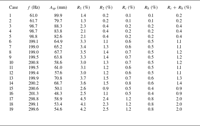
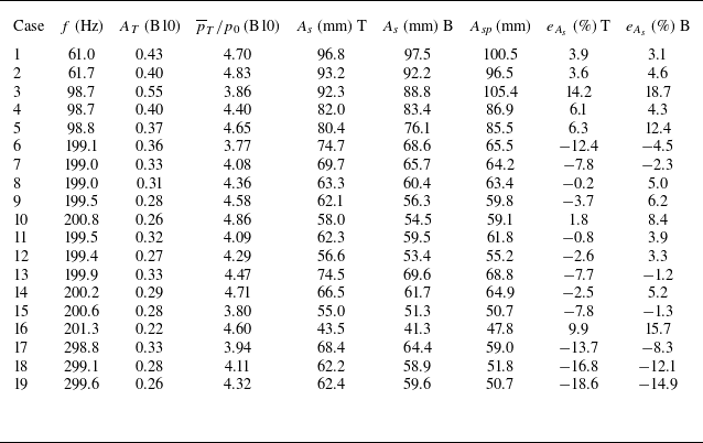
is quantitatively evaluated. The original equation is
 \begin{equation} k_{1}\left(\overline {x}u^{\prime 2}+2\overline {u}_{0}u^{\prime }x^{\prime }+\overline {u}_{0}^{2}x^{\prime }\right)=p_{T}^{\prime }=A_T\overline {p}_{T}\sin (\omega t), \end{equation}
which can be further expressed as
 \begin{equation} c_1\left (\frac {{\rm d}x^{\prime }}{{\rm d}t}\right )^2+c_2\left (\frac {{\rm d}x^{\prime }}{{\rm d}t}\right )+c_3x^{\prime }=c_4\sin (\omega t) \end{equation}
with
 \begin{equation} c_1 = k_1 \overline {x},\quad c_2 = 2k_1 \overline {u}_0 \overline {x},\quad c_3 = k_1 \overline {u}_0^2,\quad c_4 = A_T \overline {p}_T, \end{equation}
where
 $c_1$
is the nonlinear term coefficient,
 $c_2$
and
 $c_3$
are the linear term coefficients and
 $c_4$
is the excitation term coefficient.
Since
 $\varepsilon =c_1/c_2=8.2\times 10^{-4}\ll 1$
, the system is weakly nonlinear. The nonlinear term is a continuous function of
 $\varepsilon$
, and the linear system has a well-defined solution. Therefore, the regular perturbation method can be used to quantitatively evaluate the nonlinear term (Hinch Reference Hinch1991).
Specifically, for a system containing a small parameter
 $\varepsilon$
, the solution can be expanded as a power series:
 \begin{equation} x^{\prime }(t) = {x_0}^{\prime }(t) + \varepsilon {x_1}^{\prime }(t) + {\varepsilon ^2}{x_2}^{\prime }(t) + \cdots .\end{equation}
Thus,
 \begin{equation} \frac {{{\rm d}x'}}{{{\rm d}t}} = \frac {{{\rm d}{x_0}^{\prime}}}{{{\rm d}t}} + \varepsilon \frac {{{\rm d}{x_1}^{\prime}}}{{{\rm d}t}} + {\varepsilon ^2}\frac {{{\rm d}{x_2}'}}{{{\rm d}t}} + \cdots .\end{equation}
Squaring both sides yields
 \begin{align} {\left(\frac {{{\rm d}x'}}{{{\rm d}t}}\right)^2} = {\left(\frac {{{\rm d}{x_0}^{\prime}}}{{{\rm d}t}} + \varepsilon \frac {{{\rm d}{x_1}^{\prime}}}{{{\rm d}t}} + \cdots \right)^2} &= {\left ( {\frac {{{\rm d}{x_0}^{\prime}}}{{{\rm d}t}}} \right )^2} + 2\varepsilon \frac {{{\rm d}{x_0}^{\prime}}}{{{\rm d}t}}\frac {{{\rm d}{x_1}^{\prime}}}{{{\rm d}t}}\nonumber\\&\quad + {\varepsilon ^2}\left [ {{{\left ( {\frac {{{\rm d}{x_1}^{\prime}}}{{{\rm d}t}}} \right )}^2} + 2\frac {{{\rm d}{x_0}^{\prime}}}{{{\rm d}t}}\frac {{{\rm d}{x_2}'}}{{{\rm d}t}}} \right ] + \cdots .\end{align}
Substituting into (A2) gives
 \begin{align} &\varepsilon \left[{\left(\frac {{{\rm d}{x_0}^{\prime}}}{{{\rm d}t}}\right)^2} + 2\varepsilon \frac {{{\rm d}{x_0}^{\prime}}}{{{\rm d}t}}\frac {{{\rm d}{x_1}^{\prime}}}{{{\rm d}t}} + \cdots \right] + \left(\frac {{{\rm d}{x_0}^{\prime}}}{{{\rm d}t}} + \varepsilon \frac {{{\rm d}{x_1}^{\prime}}}{{{\rm d}t}} + \cdots \right) + \frac {{{c_3}}}{{{c_2}}}\bigl({x_{0}}' + \varepsilon {x_1}^{\prime} + \cdots \bigr)\nonumber\\&\quad = \frac {{{c_4}}}{{{c_2}}}\sin (\omega t). \end{align}
Since
 $\varepsilon$
is small, higher-order correction terms decay rapidly, so a first-order approximation is sufficient. Organising by powers of
 $\varepsilon$
yields the zeroth-order and first-order equations.
For the zeroth-order equation (
 $\varepsilon ^0$
), which is the linear differential equation in this work:
 \begin{equation} \frac {{{\rm d}{x_0}^{\prime}}}{{{\rm d}t}} + \frac {{{c_3}}}{{{c_2}}}{x_0}^{\prime} = \frac {{{c_{4}}}}{{{c_2}}}\sin (\omega t). \end{equation}
Its steady-state solution is
 \begin{equation} {x_0}^{\prime}(t) = {A_1}\sin (\omega t + \psi ) \end{equation}
with
 \begin{equation} {A_1} = \frac {{{c_4}}}{{\sqrt {{c_2}^2{\omega ^2} + {c_3}^2} }},\quad \psi = - \arctan \frac {{{c_2}\omega }}{{{c_3}}}. \end{equation}
The solution is consistent with (4.15), where
 $A_s=2A_1$
. The results obtained from transducers B11 are used for subsequent analysis (see § 4.2).
For the first-order equation (
 $\varepsilon ^1$
), which describes the correction arising from the nonlinear term:
 \begin{equation} \frac {{{\rm d}{x_1}^{\prime}}}{{{\rm d}t}} + \frac {{{c_3}}}{{{c_2}}}{x_1}^{\prime} = - {\left(\frac {{{\rm d}{x_0}^{\prime}}}{{{\rm d}t}}\right)^2}. \end{equation}
The right-hand side is equal to
 \begin{equation} {\left(\frac {{{\rm d}{x_0}^{\prime}}}{{{\rm d}t}}\right)^2} = {A_1}^2{\omega ^2}\cos ^2(\omega t + \psi ) = \frac {{{A_1}^2{\omega ^2}}}{2}[1 + \cos (2\omega t + 2\psi )]. \end{equation}
Substituting into (A11):
 \begin{equation} \frac {{{\rm d}{x_1}^{\prime}}}{{{\rm d}t}} + \frac {{{c_3}}}{{{c_2}}}{x_1}^{\prime} = - \frac {{{A_1}^2{\omega ^2}}}{2} - \frac {{{A_1}^2{\omega ^2}}}{2}\cos (2\omega t + 2\psi ). \end{equation}
Its steady-state solution is
 \begin{equation} {x_{1}}'(t) = E + F\cos (2\omega t + 2\psi ) + G\sin (2\omega t + 2\psi ) \end{equation}
with
 \begin{equation} E = - \frac {{{A_1}^2{\omega ^2}{c_2}}}{{2{c_3}}},\quad F = - \frac {{{A_1}^2{\omega ^2}}}{2}\frac {{{c_2}{c_3}}}{{4{\omega ^2}{c_2}^2 + {c_3}^2}},\quad G = - \frac {{{A_1}^2{\omega ^2}}}{2}\frac {{2\omega {c_2}^2}}{{4{\omega ^2}{c_2}^2 + {c_3}^2}}. \end{equation}
Combining the two solutions above and considering the first-order approximation yields
 \begin{align} x'(t) \approx {x_0}^{\prime}(t) + \varepsilon {x_1}^{\prime}(t) &= {A_1}\sin (\omega t + \psi ) + \varepsilon \left [ E + F\cos (2\omega t + 2\psi )\right. \nonumber\\&\quad\left . +\, G\sin (2\omega t + 2\psi ) \right ]\!. \end{align}
Since this paper focuses on the oscillation amplitude, our quantitative assessment compares the amplitudes of the relevant terms only. By disregarding phase differences, this approach yields a conservative upper bound on the nonlinear contribution.
First, comparing the nonlinear term on the left-hand side of (A2) with each linear term yields two ratios:
 \begin{align} {R_1} &= \frac {{{c_1}{A_1}\omega }}{{{c_2}}} = \frac {{{A_1}\omega }}{{2{{\overline u }_0}}} ,\end{align}
 \begin{align} {R_2} &= \frac {{{c_1}{A_1}{\omega ^2}}}{{{c_3}}} = \frac {{{A_1}{\omega ^2}\overline x }}{{\overline u _0^2}}. \end{align}
As summarised in table 4, under various experimental conditions the maximum values of
 $R_1$
and
 $R_2$
are 4.5 % and 2.5 %.
Ratio of nonlinear to linear terms obtained from the B11 pressure transducer.

Next, we consider the impact of the nonlinear term on the final solution obtained from the perturbation analysis.
The constant term of the first-order correction is
 \begin{equation} E = - \frac {{{A_1}^2{\omega ^2}{c_2}}}{{2{c_3}}} = - \frac {{{A_1}^2{\omega ^2}\overline x }}{{{{\overline u }_0}}}. \end{equation}
Compared with the solution of zeroth-order equations, the relative magnitude of the constant term is
 \begin{equation} {R_c} = \frac {{\varepsilon \left | E \right |}}{{{A_1}}} = \frac {{{A_1}{\omega ^2}\overline x }}{{2\overline u _0^2}}. \end{equation}
The maximum value of
 $R_c$
is 1.2 %.
Now consider the second-harmonic term of the first-order correction:
 \begin{equation} F\cos (2\omega t + 2\psi ) + G\sin (2\omega t + 2\psi ). \end{equation}
Its relative magnitude is
 \begin{equation} {R_h} = \frac {{\varepsilon \sqrt {{F^2} + {G^2}} }}{{{A_1}}}. \end{equation}
Prediction results of shock-train-motion amplitude on top and bottom wall sides using the B10 pressure transducer.

The maximum value of
 $R_h$
is 0.8 %.
The total proportion of the first-order correction can be approximated by the sum of the two, giving a maximum of approximately 2.0 %.
In summary, this theoretical and quantitative assessment confirms that the nonlinear effects under the current experimental conditions represent only a minor perturbation – contributing at most
 $\sim$
2 % to the predicted amplitude – within an otherwise linearly dominant system. Therefore, neglecting these terms to simplify the model is both reasonable and robust for the present study. The derived formulas (e.g.
 $R_1$
,
 $R_2$
,
 $R_c$
,
 $R_h$
) also provide general criteria for estimating the relative magnitude of nonlinear effects, which can guide the applicability of the linear model for other operating conditions.
Appendix B. Further validation of the prediction model
Further analysis of the pressure data under various operating conditions reveals that the B10 transducer has also consistently been located downstream of the leading shock. Therefore, we use this transducer to further validate the model. This can further verify the impact of selecting the flow direction position of the transducer on the prediction results (figure 20). As shown in table 5, the absolute error ranges from
 $-$
11.6 to 16.6 mm, and most of the relative errors are also within
 $\pm 15\,\%$
, which is close to the prediction error using B11 transducer (figure 14). In addition, as the shock train moves to different positions, the relative size of the separation bubbles behind the leading shock changes (figure 5), along with the self-excited oscillation characteristics of the shock train (figure 9). This introduces uncertainty in the amplitude difference of the leading-shock movement between the top and bottom walls. Consequently, although the prediction model relies on the linear pressure profile of the bottom wall, the predicted values for the bottom wall may not be more accurate than those for the top wall.
Statistics of experimental and predicted results using B10 transducer.

Appendix C. Determination of leading-shock positions
Given the mean backpressure, pressure oscillation amplitude and pressure oscillation frequency at the B10 or B11 transducer, the most upstream and downstream positions of the leading shock can be determined through the following steps.
-
(i) The average position difference between the leading shocks on the top and bottom walls is calculated for different steady backpressures.
-
(ii) Given the average backpressure at the outlet, along with the incoming flow velocity
$\overline {u}_0$
and
$k_1$
value, the average position of the leading shock
$\overline {x}$
(bottom wall) can be determined using (4.3). Alternatively, it can also be estimated through linear interpolation of experimental results under steady backpressures. -
(iii) The average position of the leading shock on the top wall can be determined by combining
$\overline {x}$
and the average position difference between the leading shocks on the top and bottom walls. -
(iv) Given the mean backpressure at the outlet, pressure oscillation amplitude and pressure oscillation frequency, along with the previously obtained
$k_1$
and
$\overline {x}$
values, the oscillation amplitude of the shock train can be obtained by using (4.15). -
(v) Based on the average positions of the leading shocks on the top and bottom walls (steps (ii) and (iii)), the most upstream and downstream positions of the leading shock at each wall can be determined by adding and subtracting half of the shock-train-oscillation amplitude (step (iv)).