1. Introduction
Richtmyer–Meshkov instability (RMI) occurs when a perturbed interface separating two substances of different densities is accelerated by a shock wave (Richtmyer Reference Richtmyer1960; Meshkov Reference Meshkov1969). Baroclinic vorticity and pressure perturbation are widely recognized as the two primary driving forces behind this instability (Brouillette Reference Brouillette2002). The baroclinic vorticity arises from the misalignment of pressure and density gradients across the perturbed interface, while pressure perturbations are induced by the perturbed waves resulting from shock–interface interaction. The RMI plays a crucial role in various important engineering and scientific fields, such as inertial confinement fusion (ICF) (Nuckolls et al. Reference Nuckolls, Wood, Thiessen and Zimmerman1972; Lindl, McCrory & Campbell Reference Lindl, McCrory and Campbell1992; Betti & Hurricane Reference Betti and Hurricane2016; Zylstra et al. Reference Zylstra2022), scramjet (Yang, Kubota & Zukoski Reference Yang, Kubota and Zukoski1993; Urzay Reference Urzay2018) and supernova explosion (Arnett et al. Reference Arnett, Bahcall, Kirshner and Woosley1989; Kuranz et al. Reference Kuranz2018). As a result, RMI has received extensive attention for decades (Zhou Reference Zhou2017a
,Reference Zhou
b
; Zhou et al. Reference Zhou2019; Zhou Reference Zhou2024). In ICF, perturbation evolution and material mixing induced by hydrodynamic instabilities, primarily RMI and Rayleigh–Taylor instability (Rayleigh Reference Rayleigh1883; Taylor Reference Taylor1950), have detrimental effects on the realization of high-gain ignition (Zhou, Sadler & Hurricane Reference Zhou, Sadler and Hurricane2025). Note that the RMI effect on the implosion performance is strongly dependent on the target design (Kritcher et al. Reference Kritcher2022). A typical single-shell target is composed of a low-Z ablative layer and a deuterium–tritium fuel layer (Lindl Reference Lindl1995; Kritcher et al. Reference Kritcher2022). In contrast, a double-shell target, which allows for a higher fuel pressure at a lower shell convergence (Amendt et al. Reference Amendt, Colvin, Tipton, Hinkel, Edwards, Landen, Ramshaw, Suter, Varnum and Watt2002, Reference Amendt2007, Reference Amendt, Milovich, Perkins and Robey2010), comprises a low-Z ablative layer, a low-density foam cushion, a high-Z inner shell and a mid-Z tamper layer surrounding deuterium–tritium fuel (Amendt et al. Reference Amendt, Colvin, Tipton, Hinkel, Edwards, Landen, Ramshaw, Suter, Varnum and Watt2002; Merritt et al. Reference Merritt2019; Schmidt et al. Reference Schmidt2023). Additionally, the materials used in the various layers of different targets exhibit significant diversity (Lindl et al. Reference Lindl, Landen, Edwards and Moses2014). Therefore, the Atwood numbers (
 $A=(\rho _{\textrm {d}}-\rho _{\textrm {u}})/(\rho _{\textrm {d}}+\rho _{\textrm {u}})$
, where
 $\rho _{\textrm {d}}$
and
 $\rho _{\textrm {u}}$
represent the densities of substances downstream and upstream of the interface, respectively) of the interfaces present in ICF targets vary significantly. In our previous work (Chen et al. Reference Chen, Xing, Wang, Zhai and Luo2023), RMI at a light–heavy interface (
 $\rho _{\textrm {u}}\lt \rho _{\textrm {d}}$
), referred to as L-H RMI, over a wide range of
 $A$
conditions has been comprehensively studied. However, heavy–light interfaces (
 $\rho _{\textrm {u}}\gt \rho _{\textrm {d}}$
) are more common in various types of ICF targets. Therefore, it is imperative to explore the Atwood-number dependence of RMI at a heavy–light interface (H-L RMI). Because the present study focuses on compressible RMI,
 $A$
hereafter generally refers to the post-shock Atwood number (
 $A_1$
), which contains information about flow compressibility, instead of the pre-shock one (
 $A_0$
).
For a shocked interface with a small initial amplitude (
 $ka_{0}$
, where
 $k$
and
 $a_{0}$
are the perturbation wavenumber and initial amplitude, respectively), its amplitude evolution first undergoes a start-up process, i.e. the amplitude growth rate (
 $\dot {a}$
) rises from zero and gradually reaches an asymptotic value (
 $\dot {a}_{l}$
) (Richtmyer Reference Richtmyer1960; Yang, Zhang & Sharp Reference Yang, Zhang and Sharp1994). The interface amplitude increases as the start-up process begins in the L-H RMI. However, for a shocked heavy–light interface, its amplitude first decreases with time, becoming zero and then increases reversely. This process is referred to as phase inversion (Yang, Zhang & Sharp Reference Yang, Zhang and Sharp1994; Li et al. Reference Li, Chen, Zhai and Luo2024), which starts at the onset of the shock impact and ends when the amplitude becomes zero. Lombardini & Pullin (Reference Lombardini and Pullin2009) proposed an analytical model to forecast the characteristic time of the start-up process in L-H RMI flows. For H-L RMI, Yang et al. (Reference Yang, Zhang and Sharp1994) first proposed a linear compressible theory (YZS theory) to predict the perturbation evolution in the start-up period. However, this theory requires numerical solutions. Recently, following the approach of Lombardini & Pullin (Reference Lombardini and Pullin2009), Li et al. (Reference Li, Chen, Zhai and Luo2024) constructed an analytical model (Li model) to predict the amplitude evolution of H-L RMI in the start-up period. As the waves propagate and evolve, compressibility weakens, and the perturbation evolution enters the linear phase where nonlinearity remains limited. For this period, Richtmyer (Reference Richtmyer1960) first proposed a semi-empirical model, known as the impulsive model, to predict
 $\dot {a}_{l}$
of L-H RMI. Subsequently, Meyer & Blewett (Reference Meyer and Blewett1972) constructed an empirical model (MB model) for forecasting
 $\dot {a}_{l}$
of H-L RMI on the basis of numerical simulations and the impulsive model. Through considering tangential velocities at the interface and bulk vorticity, Wouchuk & Nishihara (Reference Wouchuk and Nishihara1996, Reference Wouchuk and Nishihara1997) proposed an analytical solution (WN model) to predict
 $\dot {a}_{l}$
in both L-H and H-L RMI. Under the weak shock limit, the bulk vorticity is negligible and the WN model can be simplified to an irrotational version (WNi model) (Wouchuk & Nishihara Reference Wouchuk and Nishihara1997; Wouchuk Reference Wouchuk2001).
As nonlinearity becomes significant,
 $\dot {a}$
decreases gradually, and the perturbation evolution enters the nonlinear stage. In recent systematic reviews (Zhou Reference Zhou2017a
, Reference Zhou2024), most existing nonlinear models were introduced and classified into three types based on their derivation methods. Referring to the model type categorization of Zhou (Reference Zhou2017a
, Reference Zhou2024), we briefly review the representative nonlinear models here. The first type of model can be referred to as the Pad
 $\acute {\text {e}}$
approximation model. An early representative Padé approximation model was proposed by Zhang & Sohn (Reference Zhang and Sohn1997a
). The perturbation expansion method was first employed to derive the perturbation series of the amplitude growth rates of spike, bubble and entire interface. Then, to extend the valid range of the perturbation series, which are in the form of polynomials of time, single-point Padé approximation was employed, which yields an approximate nonlinear solution known as the ZS model. Subsequently, to realize the prediction of perturbation evolution at later times, Zhang, Deng & Guo (Reference Zhang, Deng and Guo2018) proposed a new Padé approximation model (ZDG model) by using the two-point Padé approximation. Although this model needs to be solved numerically, it is valid at asymptotically large times. Note that by considering high-order perturbation series and employing high-order Padé approximations, Velikovich & Dimonte (Reference Velikovich and Dimonte1996) and Velikovich, Herrmann & Abarzhi (Reference Velikovich, Herrmann and Abarzhi2014) realized the prediction of nonlinear perturbation evolution using a similar idea. The second type of model is referred to as the potential flow model, which is based on the potential flow modelling approach pioneered by Layzer (Reference Layzer1955). In recent years, the development of the potential flow model has made remarkable progress. Zhang & Guo (Reference Zhang and Guo2016) studied the late-time asymptotic behaviour of RMI by considering the governing equations for incompressible, inviscid and irrotational fluids with arbitrary density ratios in two dimensions (Layzer Reference Layzer1955) and first derived the late-time asymptotic finger (bubble and spike) growth rate. Then, by matching the early- and late-time solutions, a nonlinear model known as the ZG model was obtained. On the basis of the ZG model, Zhang & Guo (Reference Zhang and Guo2022) recently proposed a new nonlinear model (ZG-New model) by additionally considering the weakly nonlinear and pre-asymptotic behaviours. The third type of nonlinear model is the heuristic model, proposed by matching the early-time linear and late-time nonlinear solutions. Sadot et al. (Reference Sadot, Erez, Alon, Oron, Levin, Erez, Ben-Dor and Shvarts1998) proposed a heuristic model (SEA model) by matching the impulsive model prediction, second-order perturbation expansion solution and potential flow solution. Afterwards, based on the extension of Layzer’s theory (Layzer Reference Layzer1955) to arbitrary
 $|A_{1}|$
conditions (Goncharov Reference Goncharov2002), Mikaelian (Reference Mikaelian2003) proposed a heuristic model (MIK model) for bubble evolution, which assumes that the amplitude growth enters the nonlinear regime when
 $ka=1/3$
. Despite the limitations of the method to generalize the MIK model to spike (Jacobs & Krivets Reference Jacobs and Krivets2005), it is still interesting to evaluate its capability of predicting spike evolution because of its simplicity (Dimonte & Ramaprabhu Reference Dimonte and Ramaprabhu2010). On the basis of previous models (Zhang & Sohn Reference Zhang and Sohn1997a
; Sadot et al. Reference Sadot, Erez, Alon, Oron, Levin, Erez, Ben-Dor and Shvarts1998; Mikaelian Reference Mikaelian2003) and numerous simulations, Dimonte & Ramaprabhu (Reference Dimonte and Ramaprabhu2010) proposed a heuristic model (DR model) applicable to high-
 $|A_{1}|$
and high-initial-amplitude conditions. In our recent work (Chen et al. Reference Chen, Xing, Wang, Zhai and Luo2023), based on experimental data, we constructed a new empirical model (mDR model) by modifying the DR model, which is capable of predicting the weakly nonlinear amplitude evolution of RMI with
 $A_{1}$
ranging from 0.30 to 0.86.
Experimentally, Meshkov (Reference Meshkov1969) first studied H-L RMI using a nitrocellulose membrane to separate gases of different densities, considering
 $A_0$
ranging from −0.50 to −0.91. However, there was no available quantitative model for comparison at that time. Using a thin plastic or nitrocellulose membrane to separate gases, Houas & Chemouni (Reference Houas and Chemouni1996) performed experiments on H-L RMI with
 $A_{1}$
ranging from −0.14 to −0.83, aiming to study the thickness growth of the turbulent mixing zone. The thickness evolution of the turbulent mixing zone was found to fall in a range delimited by the linear and the
 $t^{2/3}$
power law theories, with a weak tendency towards the latter. In addition, the diaphragm was observed to also influence the mixing process. Using interfaces formed by a microfilm membrane, Jourdan & Houas (Reference Jourdan and Houas2005) experimentally studied H-L RMI with high-initial-amplitude perturbations in a large-cross-section horizontal shock tube. The phase-inversion process in H-L RMI with low
 $|A_{1}|$
(
 $=0.05$
) was accurately predicted by the impulsive model. Furthermore, the nonlinear amplitude evolution in the case with relatively high
 $|A_{1}|$
(
 $=0.77$
) is well described by the analytic model of Vandenboomgaerde & Lafitte (Reference Vandenboomgaerde, Lafitte and Dalziel2004) balanced by a reduction factor proposed by Rikanati et al. (Reference Rikanati, Oron, Sadot and Shvarts2003). Mariani et al. (Reference Mariani, Vandenboomgaerde, Jourdan, Souffland and Houas2008) conducted experiments on RMI at an air–helium (HE) interface (
 $A_{1}\approx -0.764$
), with gas separation through a thin nitrocellulose membrane deposited on a stereolithographed grid support. The experimental results are in excellent agreement with theories (Richtmyer Reference Richtmyer1960; Vandenboomgaerde, Gauthier & Mugler Reference Vandenboomgaerde, Gauthier and Meégler2002) and simulations, probably because the effect of the membrane on flow evolution is limited in the heavy–light configuration.
To avoid the influence of membrane fragments and supporting grids on interface evolution, Puranik et al. (Reference Puranik, Oakley, Anderson and Bonazza2004) first used a sinusoidal plate to separate the driven gas (CO
 $_2$
) from the test gas (air), and then withdrew it to create a membrane-less heavy–light interface with
 $A_{1}=-0.249$
. The perturbations grow rapidly after phase inversion for approximately 700 μs. Subsequently,
 $\dot {a}$
decreases and the interface evolution is dominated by interactions between adjacent mushroom-like structures, resulting in localized turbulent mixing. However, the sinusoidal plate drags a small amount of fluid that then bounces back from the shock-tube wall as gravity waves. Additionally, the perturbation begins to evolve after plate withdrawal due to the Rayleigh–Taylor instability, resulting in a non-stationary initial interface. Furthermore, the diffusion layer of this membrane-less gaseous interface may also affect the instability behaviour. By dropping a two-liquid system mounted on a sled onto a coil spring to produce a nearly impulsive upward acceleration, Niederhaus & Jacobs (Reference Niederhaus and Jacobs2003) studied incompressible H-L RMI on a membrane-less liquid interface with low
 $|A_{1}|$
(
 $=0.1587$
). The flow evolution was recorded using planar laser-induced fluorescence imaging. An excellent agreement between the experimental
 $\dot {a}_{l}$
and its theoretical counterpart, determined by integrating the first-order time derivative of the impulsive model, was reached for a dimensionless time up to 0.3.
Using the soap-film technique to generate single-mode SF
 $_6$
–air interfaces free of solid membrane, supporting grid and diffusion layer, Guo et al. (Reference Guo, Cong, Si and Luo2022) conducted shock-tube experiments on the evolution of H-L RMI with
 $A_{1}=-0.578$
. It was found that the MB and ZG models accurately predict the linear and nonlinear amplitude evolutions, respectively. Recently, additional shock-tube experiments employing the soap-film technique, with
 $A_{1}$
ranging from −0.72 to −0.62, were performed to explore the effects of high initial amplitude and compressibility on H-L RMI (Wang et al. Reference Wang, Wang, Zhai and Luo2023; Li et al. Reference Li, Chen, Zhai and Luo2024). The MB model was observed to be less accurate in predicting
 $\dot {a}_{l}$
when
 $ka_{0}$
is high or the incident shock is strong. In addition, the Li model was found to be capable of predicting the start-up evolution under various shock intensity conditions. Overall, previous experimental works have focused on H-L RMI with a single
 $A_{1}$
or similar
 $A_{1}$
. While these studies offer valuable insights, desirable experimental research on H-L RMI over a wide range of
 $A_{1}$
conditions remains lacking. With the rapid development of computing power and the advances in algorithms, numerical simulation has become a powerful tool for studying RMI (Zhou Reference Zhou2017a
,Reference Zhou
b
; Zhou et al. Reference Zhou2019; Zhou Reference Zhou2024). Existing numerical works (Nishihara et al. Reference Nishihara, Wouchuk, Matsuoka, Ishizaki and Zhakhovsky2010; Thornber et al. Reference Thornber, Drikakis, Youngs and Williams2010; Lombardini et al. Reference Lombardini, Hill, Pullin and Meiron2011) have provided valuable insights into the evolution law of RMI under various
 $A_{1}$
conditions, which should be further verified via experiments. Therefore, it is desirable to conduct a fine and systematic experimental study on the Atwood-number dependence of H-L RMI.
In this work, evolutions of H-L RMI under diverse
 $A_{1}$
conditions are first experimentally obtained using an improved soap-film technique. Subsequently, the predictive capabilities of a model describing the start-up stage, empirical and analytical linear models, and some representative nonlinear models are evaluated through comparative analysis with experimental results. Finally, based on experimental data and existing models, an empirical nonlinear model applicable to describe the weakly nonlinear evolution of RMI over a wide range of
 $A_{1}$
conditions is proposed.
2. Experimental methods
Sketch of the shock tube and high-speed schlieren system.

The experiments are performed in a horizontal shock tube, as shown in figure 1. The tube consists of a driver section, a driven section, a transitional section, two stable sections (I and II) and a test section. The method of shock generation and the thickness of the polyester film used to separate gases in the driver and driven sections are consistent with those used in previous work (Chen et al. Reference Chen, Xing, Wang, Zhai and Luo2023) and are kept consistent across all experiments. This ensures that the shock intensity (defined as
 $S=1-p_{in}/p_{be}$
, where
 $p_{in}$
and
 $p_{be}$
represent the pressures of fluids in front of and behind the incident shock, respectively) remains similar across different experiments.
The soap-film technique widely utilized and verified in prior studies (Liu et al. Reference Liu, Liang, Ding, Liu and Luo2018; Liang et al. Reference Liang, Zhai, Ding and Luo2019; Luo et al. Reference Luo, Liang, Si and Zhai2019) is employed to generate the initial interface. The transparent soap-film-forming devices (u and d) as depicted in figure 2 are manufactured by combining two acrylic plates with pedestals. More details on the soap-film formation are available in previous works (Liu et al. Reference Liu, Liang, Ding, Liu and Luo2018; Liang et al. Reference Liang, Zhai, Ding and Luo2019) and are omitted here for brevity. To realize a wide range variation of
 $A_{1}$
, air on both sides of the soap film should be replaced with different gases. The gas replacement procedures are as follows. First, a thin aluminium membrane is attached to the left side of stable section II to separate it from stable section I. Second, a light gas such as Kr or He is charged through the inflow hole into device d, whose left and right sides are sealed by the soap film and polyester film, respectively, while air is released through the outflow hole. Third, devices u and d are carefully connected and inserted into the test section. Fourth, a heavy gas such as SF
 $_{6}$
or C
 $_{4}$
F
 $_{10}$
is charged slowly into the region between the aluminium membrane and soap film through the inlet pipe and air is released through the outlet pipe. An oxygen concentration detector is placed at the outlet pipe to monitor the oxygen concentration upstream of the soap film. Once the volume fraction of oxygen drops below 0.5
 $\%$
, the pipes are removed and the holes are sealed. Notably, in the experiment with an air–He interface (a SF
 $_{6}$
–air or C
 $_{4}$
F
 $_{10}$
–air interface), the first and fourth procedures (the second procedure) will be skipped. Since the gas in device d (gas d) is lighter than that in device u (gas u), a heavy–light single-mode interface is naturally formed. Note that the height of the test section is 6.00 mm. There are two reasons for choosing such a small value for the test section height. First, this reduces the ratio of the interface height to perturbation wavelength (
 $\lambda$
: 40.00 mm in present experiments), thereby reducing the three-dimensionality caused by the surface tension of the soap-film interface (Luo, Wang & Si Reference Luo, Wang and Si2013). Second, this reduces the gas pressure difference at the upper and lower sides of the interface caused by gravity, thus minimizing the three-dimensionality introduced by gravity.
Schematic of interface formation devices.

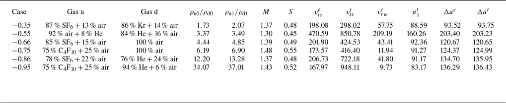
Significant parameters for six experimental cases labelled by
 $A_1$
.Superscripts ‘
 $e$
’ and ‘
 $t$
’ denote experimental and theoretical results, respectively; gases u and d: gases in devices u and d, respectively;
 $\rho _{\textrm {u0}}$
and
 $\rho _{\textrm {d0}}$
(
 $\rho _{\textrm {u1}}$
and
 $\rho _{\textrm {d1}}$
): pre-shock (post-shock) densities of gases u and d, respectively;
 $M$
: Mach number of the incident shock encountering the heavy–light single-mode interface;
 $S=1-p_{in}/p_{be}$
: shock strength, with
 $p_{in}$
and
 $p_{be}$
being the pressures of gases in front of and behind the incident shock, respectively;
 $v_{is}$
,
 $v_{ts}$
and
 $v_{rw}$
: velocities of the incident shock, transmitted shock and average position of the reflected rarefaction waves, respectively;
 $u_{1}$
: velocity of gas u behind the incident shock;
 $\Delta u$
: shock-induced interface velocity. The unit of velocity is m s
 $^{-1}$
, and similarly hereafter.

The flow evolution is recorded using a high-speed schlieren system as depicted in figure 1. The high-speed video camera (FASTCAM SA5, Photron Limited) operates at a frame rate of 50 000 frames per second, with an exposure time of 1 μs. The spatial resolution of schlieren images is approximately 0.35 mm pixel
 $^{-1}$
. The ambient pressure and temperature are
 $101.3\pm 0.1$
kPa and
 $296.5\pm 1.5$
K, respectively.
To highlight the effect of
 $A_1$
on the evolution law, six experiments with different
 $A_1$
but same
 $|ka_{0}|$
(0.27) and
 $\lambda$
(40.00 mm) are conducted. Note that
 $a_0$
is defined to be negative, and the case with
 $A_{1}=f$
is referred to as case
 $f$
hereafter. The significant parameters for the six cases are provided in table 1. The gas concentrations on both sides of the interface are determined using a MATLAB procedure that solves the shock–interface interaction based on one-dimensional gas dynamics theory. The specific processes are as follows. First, the velocities of the incident shock (
 $v_{is}$
), transmitted shock (
 $v_{ts}$
) and shocked interface (
 $\Delta u$
) are measured from experiments, with the experimental
 $v_{is}$
input into the MATLAB procedure as a fixed initial condition. Next, the volume fractions of heavy gas upstream and light gas downstream of the initial interface are adjusted to match the experimental
 $v_{ts}$
with its theoretical counterpart, while also ensuring that the experimental
 $\Delta u$
(
 $\Delta u^e$
) is in reasonable agreement with its theoretical counterpart (
 $\Delta u^t$
). Once these two objectives are achieved, the volume fractions of gases used in the procedure are considered the corresponding experimental values. As shown in table 1,
 $\Delta u^e$
and
 $\Delta u^t$
are in excellent agreement, indicating that the determination of the gas concentrations on both sides of the interface is reliable. Since the physical properties of gas u in different cases are diverse, the Mach number of the incident shock impacting the heavy–light single-mode interface (
 $M$
) varies between cases. However, the shock strengths
 $S$
remain similar across all experiments. It is noteworthy that the highest
 $|A_1|$
reached in the present work is 0.95, which, to our knowledge, exceeds that in any previous experiment with a gaseous interface.
3. Results and discussion
3.1. Flow features and interface morphology
Experimental schlieren photographs of the evolutions of shocked heavy–light single-mode interfaces with different
 $A_{1}$
. Numbers represent time in microseconds.

Experimental schlieren images of the evolutions of shocked heavy–light single-mode interfaces with different
 $A_1$
are shown in figure 3. Case −0.66 is taken as an example to illustrate the detailed evolution process. The temporal origin (
 $t = 0$
μs) is defined as the moment the incident shock hits the initial interface. It is noteworthy that the initial interface appears thick due to the sinusoidal strips embedded in the interface formation device for constraining the soap film. For clarity, the shadows from these strips are removed from the images through image processing once the shocked interface has moved away. Moreover, the width of the shocked interface in the experimental schlieren images generally increases over the evolution process. This phenomenon is primarily attributed to the gradual detachment of broken soap-film droplets from the interface, resulting in a relatively significant density gradient in the flow field adjacent to the interface. When the incident shock impacts the initial interface, a transmitted shock wave and reflected rarefaction waves, moving downstream and upstream, respectively, are generated. The phase inversion of the shocked interface has been completed at
 $t=139$
μs. After the phase inversion, the amplitude and asymmetry of the shocked interface increase gradually (139–759 μs), followed by the formation of distinct spike and bubble structures (759 μs), indicating the generation of high-order harmonics. A comparison of experiments with different
 $A_1$
reveals that the nonlinear features of the interface evolution, such as spike and bubble structures, develop more rapidly when
 $|A_{1}|$
is higher.
Since the major interface configuration can be clearly extracted from the schlieren photographs, it is a rare opportunity to evaluate the predictive capability of perturbation solutions (Zhang & Sohn Reference Zhang and Sohn1997b
; Velikovich et al. Reference Velikovich, Herrmann and Abarzhi2014) for describing the interface shape evolution. Given the complexity of the perturbation solutions, we consider the solutions for the first four modes, with their detailed expressions available in previous works (Zhang & Sohn Reference Zhang and Sohn1997b
; Velikovich et al. Reference Velikovich, Herrmann and Abarzhi2014). Additionally, the solutions are in the form of polynomials in time and tend to diverge rapidly, hence we focus only on the early-time interface evolution. For clarity, we present the results of cases −0.35, −0.66, −0.86 and −0.95 here. Interface contours extracted from experiments (black lines) and predicted by the perturbation solutions (blue lines) are depicted in figure 4, in which
 $x=0$
and
 $y=0$
correspond to the horizontal coordinate of the mean position of the initial interface and the vertical coordinate of the tip of the bubble in the middle, respectively. For case −0.35, the perturbation solutions reasonably predict the interface shape and also the amplitude. For cases −0.66, −0.86 and −0.95, the perturbation solutions predict poorly both the interface shape and amplitude, with the discrepancies becoming more pronounced as
 $|A_1|$
increases. The failure of the perturbation solutions for cases with medium to very high
 $|A_1|$
should be attributed to that
 $\dot {a}$
is positively related to
 $|A_1|$
and these solutions diverge rapidly with the increase of
 $ka$
(Jacobs & Krivets Reference Jacobs and Krivets2005).
Interface contours extracted from experiments (black lines) and predicted by perturbation solutions (blue lines): (
 $a$
) case −0.35; (
 $b$
) case −0.68; (
 $c$
) case −0.86; (
 $d$
) case −0.95.

3.2. Amplitude evolution in start-up period
The perturbation evolution during the start-up stage establishes the initial conditions for subsequent amplitude growth. Therefore, exploring the evolution law of RMI during the start-up stage is essential. In H-L RMI, the start-up process (i.e.
 $\dot {a}$
increases gradually and reaches
 $\dot {a}_l$
when the process ends) is accompanied by the phase-inversion process (i.e. the absolute value of perturbation amplitude
 $|a|$
decreases gradually until reaching zero), both beginning at the onset of the shock impact.
Amplitude variation in the start-up period for different cases. Symbols and lines: experimental and theoretical results, respectively. Error bars represent potential errors in extracting the interface amplitude for a single experiment, with a length equal to half the width of the interface in the experimental schlieren image, and the same hereafter.

As the YZS theory (Yang et al. Reference Yang, Zhang and Sharp1994) requires numerical solutions, the analytical Li model (Li et al. Reference Li, Chen, Zhai and Luo2024) is employed to provide a theoretical reference for the amplitude evolution in the start-up period, with its expressions detailed in Appendix A for clarity. Experimental and theoretical results of the amplitude variation in the start-up period for various cases are provided in figure 5. The coordinates of the starting point of the theoretical line are (
 $t_1$
,
 $a_1$
), where
 $t_1=2|a_{0}|/v_{is}^{e}$
represents the duration of the shock–interface interaction process and
 $a_1$
is the corresponding
 $a$
at
 $t=t_1$
, with
 $v_{is}^{e}$
denoting the experimental
 $v_{is}$
. Good agreement is reached between the experimental and theoretical results, indicating that the Li model is valid for describing the start-up evolution of H-L RMI across a wide range of
 $A_1$
conditions. The phase-inversion process is completed when
 $|a|$
decreases to zero, while the end moment of the start-up process is the
 $t$
coordinate of the last point of the Li model prediction since its duration is exactly the effective prediction time of the model. According to the Li model prediction, the temporal order of the terminations of the start-up and phase-inversion processes appears to be correlated with
 $A_1$
: the start-up process terminates before (after) the phase-inversion process in cases with relatively low (high)
 $|A_1|$
, i.e. cases −0.35 and −0.55 (cases −0.66, −0.75, −0.86 and −0.95). Parameter
 $a$
varies from
 $a_1$
to 0 during the phase-inversion process. Accordingly, the relative magnitude of
 $|a_1|$
and the absolute value of the amplitude variation in the start-up process (
 $|a_{st}|$
) determine which process terminates first. Both
 $|a_{st}|$
and
 $|a_1|$
are related to
 $A_1$
,
 $S$
and specific ratios of gases u and d (
 $\gamma _{\textrm {u}}$
and
 $\gamma _{\textrm {d}}$
). However, the relationships are highly complex and nonlinear because they are correlated with parameters that need to be obtained by solving the Riemann problem, such as the velocities of waves and interface. As a result, it is challenging to specify the relationship between
 $A_1$
and the temporal order of the terminations of the start-up and phase-inversion processes and the underlying physical mechanism.
3.3. Linear amplitude evolution
According to previous studies (Yang et al. Reference Yang, Zhang and Sharp1994; Wang et al. Reference Wang, Wang, Zhai and Luo2023; Li et al. Reference Li, Chen, Zhai and Luo2024), the MB model is theoretically valid for predicting
 $\dot {a}_l$
only under conditions where
 $ka_0$
is small and compressibility is weak. In the present experiments,
 $ka_0$
satisfies the small-amplitude criterion and the shock intensity is low. Therefore, these experiments are appropriate for evaluating the MB model over a wide range of
 $A_{1}$
values. The MB model can be expressed as
 \begin{equation} \dot {a}_l^{m}=k A_{1} \Delta u^{e} a_{0}\dfrac {1+C_{c}}{2}=k A_{1} \Delta u^{e} \dfrac {a_{0}+a_{1}}{2}, \end{equation}
where
 $C_{c}=1-\Delta u^{e}/v_{is}^{e}$
is the shock compression factor. Besides the empirical MB model, it is also desirable to evaluate the analytical linear models (Wouchuk & Nishihara Reference Wouchuk and Nishihara1996, Reference Wouchuk and Nishihara1997; Wouchuk Reference Wouchuk2001). As noted by Li et al. (Reference Li, Chen, Zhai and Luo2024), the difference between the predictions of the WN and WNi models is negligible when
 $S \lt 0.6$
. Because the value of
 $S$
in all current experiments is below 0.55, only the WNi model is considered here. The detailed expression of the WNi model is provided in Appendix A.
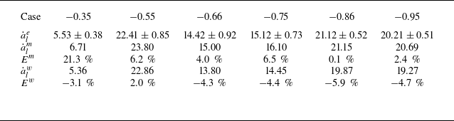
Experimental
 $\dot {a}_{l}$
(
 $\dot {a}_{l}^{e}$
), obtained by linearly fitting the amplitude evolution shortly after the start-up stage, and the theoretical counterparts predicted by the MB and WNi models (
 $\dot {a}_l^{m}$
and
 $\dot {a}_l^{w}$
) are presented in table 2 for comparison. The WNi model predicts the experimental results well under all considered
 $A_1$
conditions. In contrast, the MB model performs poorly in predicting
 $\dot {a}_{l}^{e}$
for case −0.35. Notably, the MB model was empirically developed based on numerical simulations. However, Meyer & Blewett (Reference Meyer and Blewett1972) did not consider simulations with
 $|A_1|\lt 0.5$
, which explains the MB model’s failure to predict
 $\dot {a}_{l}^{e}$
in case −0.35.
Comparison of experimental and theoretical linear amplitude growth rates. Here,
 $\dot {a}_{l}^{e}$
,
 $\dot {a}_{l}^{m}$
and
 $\dot {a}_{l}^{w}$
: linear amplitude growth rates obtained from experiments and predicted by MB and WNi models, respectively;
 $E^{m/w}=(\dot {a}_{l}^{m/w}-\dot {a}_{l}^{e})/\dot {a}_{l}^{e}$
: relative error between
 $\dot {a}_{l}^{e}$
and
 $\dot {a}_{l}^{m/w}$
. The units of linear amplitude growth rates are m s
 $^{-1}$
.

3.4. Weakly nonlinear amplitude evolution
Temporal variations of perturbation amplitude in dimensionless form for cases with different
 $A_{1}$
: (
 $a$
) overall interface; (
 $b$
) bubble and spike. Two dashed reference lines have a slope of 1 and represent the scenario where nonlinearity is absent and the bubble and spike maintain an amplitude growth rate of
 $\dot {a}_{l}^{e}$
. The increase in the length of the error bars is attributed to the gradual widening of the interface observed in the experimental schlieren images.

Temporal variations of
 $a$
and
 $a_{b/s}$
(subscripts ‘
 $b$
’ and ‘
 $s$
’ represent bubble and spike, respectively) in dimensionless form for different cases are shown in figures 6(
 $a$
) and 6(
 $b$
), respectively. Here,
 $t$
,
 $a$
and
 $a_{b/s}$
are normalized as
 $\tau =k\dot {a}_{l}^{e}(t-t^*)$
,
 $\alpha =k(a-a^*)$
and
 $\alpha _{b/s}=k(a_{b/s}-a^*_{b/s})$
, respectively, with
 $t^*$
representing the end moment of the start-up stage and
 $a^*$
(
 $a^*_{b/s}$
) being the corresponding
 $a$
(
 $a_{b/s}$
) at
 $t =t^*$
. The results of cases with
 $|A_1|\lt 0.8$
collapse onto each other but deviate from those of cases −0.86 and −0.95. This indicates that H-L RMI with
 $|A_1|\lt 0.8$
follows similar evolution laws, whereas H-L RMI with
 $|A_{1}|\gt 0.8$
exhibits significantly different behaviour. Specifically, the amplitude growth rate of the spike, which continuously decreases in cases with
 $|A_1|\lt 0.8$
, increases at the beginning of the weakly nonlinear period in cases −0.86 and −0.95. These results confirm that the spike acceleration is significant when
 $|A_{1}|$
is high, as reported in a previous numerical study (Dimonte & Ramaprabhu Reference Dimonte and Ramaprabhu2010). To our knowledge, this is the first direct experimental observation of the spike acceleration in H-L RMI. Compared to the spike, the evolution law of the bubble is less sensitive to
 $|A_1|$
, which should be attributed to the insensitivity of the asymptotic curvature of the bubble to
 $|A_1|$
(Zhang & Guo Reference Zhang and Guo2022).
For a small-initial-amplitude shocked interface, previous research (Zhou Reference Zhou2017a
,Reference Zhou
b
, Reference Zhou2024) suggests that its evolution can be approximately divided into five successive stages: start-up stage (
 $\dot {a}$
increases gradually), linear stage (
 $\dot {a}$
remains almost unvaried), weakly nonlinear stage (
 $\dot {a}$
decreases, with bubble and spike structures becoming significant), strongly nonlinear stage (roll-up structures emerge) and turbulent mixing stage (multiscale vortices appear and materials are mixed intensely). For cases with moderate to very high
 $|A_1|$
(cases −0.55, −0.66, −0.75, −0.86 and −0.95), as shown in figure 3, the asymmetry of the shocked interface increases gradually after the phase inversion, followed by the formation of distinct spike and bubble structures. This indicates that the interface evolution in these cases has entered the weakly nonlinear regime within the effective experimental time. For case −0.35, however, the shocked interface remains a quasi-single-mode profile throughout the experiment. As shown in figure 6(
 $b$
), two dashed reference lines with a slope of 1 are included for comparison. These reference lines represent the scenario where nonlinearity is absent and the bubble and spike maintain an amplitude growth rate of
 $\dot {a}_{l}^{e}$
. Both the amplitude growths of the bubble and spike deviate significantly from the reference lines at small
 $\tau$
, indicating that the interface evolution in case −0.35 has also entered the weakly nonlinear stage within the effective experimental time. Subsequently, a comparative analysis of the experimental results and predictions from typical nonlinear models is performed. Nonlinear models including the ZS, SEA, MIK, DR, ZG, ZG-New and mDR models are considered, with detailed expressions available in previous work (Chen et al. Reference Chen, Xing, Wang, Zhai and Luo2023). A comparison of the experimental and theoretical results reveals that the predictive capabilities of the considered nonlinear models for cases −0.55, −0.66 and −0.75 are highly similar. For clarity, four typical experimental cases (cases −0.35, −0.66, −0.86 and −0.95), referred to as H-L RMI with low, moderate, high and very high
 $|A_{1}|$
, respectively, are chosen for further discussion.
Comparisons between experimental and theoretical results for dimensionless
 $a$
(
 $a,c,e,g$
) and dimensionless
 $a_{b/s}$
(
 $b,d,f,h$
). (
 $a,b$
) case −0.35; (
 $c,d$
) case −0.66; (
 $e,f$
) case −0.86; (
 $g,h$
) case −0.95.

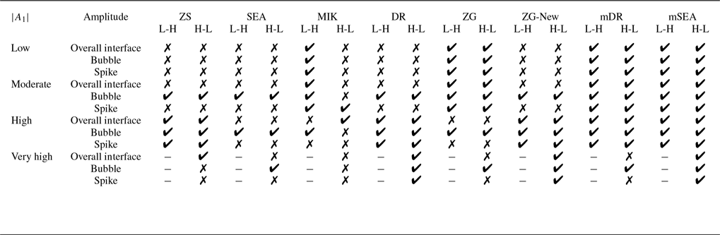
Summary of the predictive capabilities of the considered existing nonlinear models and newly proposed model (mSEA model) for the amplitude evolutions of the overall interface, bubble and spike under different
 $A_1$
conditions. L-H and H-L: L-H RMI and H-L RMI, respectively; ✔ represents that the model is capable of providing reasonable predictions for the experimental results, both theoretically and practically or coincidentally in practice; ✗ indicates that the model is practically incapable of providing a reasonable prediction;
 $-$
indicates that there are no available experimental results for comparison.

Comparisons between the temporal amplitude variations obtained from experiments and predicted by models for cases −0.35, −0.66, −0.86 and −0.95 are presented in figure 7. For case −0.35, the ZG and mDR models accurately predict the experimental results, while the other models overestimate the growths of
 $a$
and
 $a_{b/s}$
. For case −0.66, similarly, the ZG and mDR models provide accurate predictions for the experimental results. The MIK model predicts the evolutions of
 $a$
and
 $a_b$
poorly but accurately forecasts the spike evolution. In contrast, the ZS, SEA, DR, and ZG-New models provide reasonable predictions for the bubble evolution but overestimate the growths of
 $a$
and
 $a_s$
. For case −0.86, the SEA model (ZG model) overestimates (underestimates) the growths of
 $a$
and
 $a_s$
while predicting the evolution of
 $a_b$
well. The MIK model provides a reasonable prediction for the overall amplitude evolution, which is a coincidence caused by its underestimation of spike evolution and overestimation of bubble growth. In contrast, the ZS, DR, ZG-New and mDR models predict the growths of
 $a$
and
 $a_{b/s}$
accurately. For case −0.95, the SEA and mDR models (ZG model) overestimate (underestimates) the growths of
 $a$
and
 $a_s$
while accurately predicting the evolution of
 $a_b$
. The MIK model overestimates the bubble evolution while underestimating the growths of
 $a$
and
 $a_s$
. The ZS model predicts the overall amplitude evolution well, which is a coincidence caused by its overestimation of spike evolution and underestimation of bubble growth. In contrast, the DR and ZG-New models accurately predict the evolutions of
 $a$
and
 $a_{b/s}$
.
The predictive capabilities of the considered nonlinear models for L-H RMI (Chen et al. Reference Chen, Xing, Wang, Zhai and Luo2023) and H-L RMI under various
 $|A_{1}|$
conditions are summarized in table 3. It is found that only the MIK model exhibits different predictive capabilities for H-L RMI and L-H RMI under low-, moderate- and high-
 $|A_1|$
conditions. The RMI evolution can be viewed as a process that is initially compressible and subsequently becomes incompressible (Zhang & Sohn Reference Zhang and Sohn1997a
). The effect of flow compressibility on interface evolution becomes negligible when the start-up process ends (Yang et al. Reference Yang, Zhang and Sharp1994; Li et al. Reference Li, Chen, Zhai and Luo2024). Thus, the termination of the start-up stage can be regarded as the demarcation point between the compressible and incompressible periods. The origin in figure 7 represents the termination point of the start-up stage, which means the compressible period has been ‘subtracted’, and the experimental results presented include only the data in the incompressible period. In the incompressible period, both L-H RMI and H-L RMI are driven solely by baroclinic vorticity, with the major discrepancy being the difference in
 $a^*$
caused by the phase-inversion process existing in H-L RMI. For all models except the MIK model, the predictions are insensitive to
 $a^*$
, which explains why they have similar predictive capabilities for L-H RMI and H-L RMI. Notably, the analyses on their predictive capabilities for L-H RMI with low, moderate and high
 $|A_1|$
(Chen et al. Reference Chen, Xing, Wang, Zhai and Luo2023) are also applicable to H-L RMI with similar conditions, and the relevant discussions are omitted in this work. For the MIK model, one of its key assumptions is that the amplitude growth enters the nonlinear regime when
 $ka=1/3$
, i.e.
 $\dot {a}$
remains
 $\dot {a}_{l}$
when
 $ka\lt 1/3$
. Accordingly, the value of
 $ka^*$
has a significant influence on the predictions of the MIK model. In a previous study of L-H RMI (Chen et al. Reference Chen, Xing, Wang, Zhai and Luo2023), the value of
 $ka^*$
is approximately 1/3. In contrast, in the present work on H-L RMI, the value of
 $ka^*$
is much smaller than 1/3, or even negative, due to the presence of an additional phase-inversion process. This explains why the MIK model exhibits different predictive capabilities for H-L RMI and L-H RMI under low-, moderate- and high-
 $|A_1|$
conditions.
For H-L RMI with very high
 $|A_1|$
, the ZS and mDR models, which accurately describe H-L and L-H RMI with high
 $|A_1|$
, exhibit poor predictive capabilities. Under the condition of
 $|A_{1}|\gt \sqrt {(ka_{1})^{2}+1/2}\approx 0.75$
, the ZS model is derived using the
 $P^{0}_{1}$
Padé approximation. This approximation retains only a partial contribution of the third-order term of
 $a$
rather than the complete contribution. The coefficient of the neglected third-order term of
 $a$
is
 $A_{1}^{2}-1/2$
. Therefore, for RMI with
 $|A_1|\gt 0.75$
, the prediction of the ZS model is less accurate when
 $|A_{1}|$
is higher. This may explain why the ZS model predicts the results of case −0.86 well but performs poorly in predicting the amplitude evolution in case −0.95. For the mDR model constructed empirically based on experiments of L-H RMI with low to high
 $|A_1|$
, as previously mentioned (Chen et al. Reference Chen, Xing, Wang, Zhai and Luo2023), it is invalid when
 $|A_{1}|$
approaches 1 due to the limitation of the coefficient
 $E=(3-2|A_1|)/(9-9|A_1|)$
. Therefore, the failure of the mDR model under very-high-
 $|A_1|$
conditions is reasonable and foreseeable. Aside from the ZS and mDR models, the predictive capabilities of the other models for H-L RMI with very high
 $|A_1|$
are similar to those for H-L RMI with high
 $|A_1|$
, and the analyses of model predictive capabilities for the latter are also applicable to the former.
As illustrated in table 3, none of the considered models is universally applicable to RMI over the range of
 $A_{1}$
from
 $-0.95$
to
 $0.86$
. Given the complex nature of the RMI evolution, developing a rigorous theoretical model applicable over a wide range of
 $A_{1}$
conditions is challenging. Therefore, we seek to propose an empirical model based on the experimental results from the present work and the previous study on L-H RMI (Chen et al. Reference Chen, Xing, Wang, Zhai and Luo2023). To construct the empirical model, we first analyse the expressions of the existing nonlinear models. Other than the ZS and ZG-New models, the expressions of the considered nonlinear models follow a unified form:
 \begin{equation} \dot {a}_{b/s}=\dot {a}_l^e\dfrac {1+D_{b/s}k\dot {a}_l^e (t-t^*)}{1+E_{b/s}k\dot {a}_l^e (t-t^*)+F_{b/s}k^2 {\dot {a}_l^e}{}^2 (t-t^*)^2}, \end{equation}
where
 $D_{b/s}$
,
 $E_{b/s}$
and
 $F_{b/s}$
are constants or parameters related to initial conditions such as
 $|A_1|$
and
 $|a_1|$
. In the considered nonlinear models,
 $E_{b/s}$
is always non-zero, and these models can be classified into two groups according to whether
 $D_{b/s}$
and
 $F_{b/s}$
are zero. In the early stage, (3.2) could be approximated as
 \begin{equation} \dot {a}_{b/s}= \begin{cases} \dot {a}_{l}^{e}[1+(D_{b/s}-E_{b/s})k\dot {a}_{l}^{e}(t-t^*)]&\text {when } D_{b/s}\neq 0\text {, }F_{b/s}\neq 0\\ \dot {a}_{l}^{e}[1-E_{b/s}k\dot {a}_{l}^{e}(t-t^*)]&\text {when } D_{b/s}=0\text {, }F_{b/s}=0.\\ \end{cases} \end{equation}
In the late stage, (3.2) can be approximated as
 \begin{equation} \dot {a}_{b/s}= \begin{cases} \dfrac {D_{b/s}}{F_{b/s}kt}&\text {when } D_{b/s}\neq 0\text {, }F_{b/s}\neq 0\\[6pt] \dfrac {1}{E_{b/s}kt}&\text {when } D_{b/s}=0\text {, }F_{b/s}=0.\\ \end{cases} \end{equation}
When
 $D_{b/s}$
and
 $F_{b/s}$
are non-zero, the model prediction for early-time evolution is mainly influenced by
 $D_{b/s}$
and
 $E_{b/s}$
, while the model prediction of late-time interface development is primarily affected by
 $D_{b/s}$
and
 $F_{b/s}$
. In the special case where
 $D_{b/s}$
is non-zero constant,
 $E_{b/s}$
and
 $F_{b/s}$
independently govern the model predictions of the early- and late-time amplitude evolutions, respectively. Additionally, when
 $D_{b/s}$
and
 $F_{b/s}$
are zero, the evolution behaviour at both early and late stages is governed by
 $E_{b/s}$
. Notably, obtaining an empirical model which reasonably describes the Atwood-number dependence of both the early- and late-time evolution laws by modifying only one coefficient is challenging. Besides, modification based on a model with
 $D_{b/s}$
being non-zero non-constant is rather complex. Therefore, it is desirable to construct a new model on the basis of a model with
 $D_{b/s}$
being non-zero constant. The only model that satisfies these conditions is the SEA model, which is chosen as the base model for modification. The coefficients of the SEA model can be expressed as
 \begin{equation} \begin{cases} D_{b/s}^{sea}=1,&\\[5pt] E_{b/s}^{sea}=1\pm |A_{1}|,&\\[5pt] F_{b/s}^{sea}=\dfrac {1\pm |A_{1}|}{1+|A_{1}|}\dfrac {1}{2\pi C},&\\ \end{cases} \end{equation}
where
 $C=1/3\pi$
for
 $|A_{1}|\geqslant 0.5$
and
 $C=1/2\pi$
for
 $|A_{1}|\rightarrow 0$
. The upper and lower signs correspond to the bubble and spike, respectively, and similarly hereafter.
The idea of model construction is elaborated as follows. The maximum dimensionless time of experiments in the present work and previous study (Chen et al. Reference Chen, Xing, Wang, Zhai and Luo2023) does not exceed 2.5. In other words, the interface evolution in all considered experiments is within the weakly nonlinear period. Therefore, the new empirical model (mSEA model) is constructed by modifying
 $E_{b/s}^{sea}$
of the SEA model that governs the early-time evolution behaviour, while keeping the other coefficients unchanged. The SEA model overestimates the amplitude evolutions of the overall interface and spike for all present experiments with negative
 $A_1$
, consistent with the observation in previous work on RMI with positive
 $A_1$
(Chen et al. Reference Chen, Xing, Wang, Zhai and Luo2023). This should be attributed to its overestimation of the spike acceleration (Dimonte & Ramaprabhu Reference Dimonte and Ramaprabhu2010). Thus, the value of the modified
 $E_{s}^{sea}$
(
 $E_{s}^{msea}$
) needs to be larger than that of
 $E_{s}^{sea}$
under all
 $A_1$
conditions, in order to reasonably describe the evolution of spike. For the bubble, as mentioned earlier, its evolution law is less sensitive to
 $A_1$
compared with spike. Accordingly, the value of the modified coefficient
 $E_{b}^{sea}$
(
 $E_{b}^{msea}$
) should be less sensitive to
 $A_1$
compared with that of
 $E_{s}^{msea}$
. After numerous attempts,
 $E_{b,s}^{msea}$
satisfying these two requirements and also aligning with the data of all 13 experiments (with
 $A_1$
values of −0.95, −0.86, −0.75, −0.66, −0.55, −0.35, 0.30, 0.44, 0.52, 0.61, 0.68, 0.72 and 0.86) reported in the present work and prior study (Chen et al. Reference Chen, Xing, Wang, Zhai and Luo2023) is obtained as
 $(2\mp |A_{1}|)(1.07\pm |A_{1}|)$
.
As shown in figure 7, the mSEA model reasonably predicts the amplitude evolutions of H-L RMI with low, moderate, high and very high
 $|A_1|$
, and its predictive capabilities are presented in table 3 for comparison. Relatively, the mSEA model predicts bubble evolution generally better than spike development. This is because bubble evolution, which is insensitive to
 $A_1$
, is easier to model over a wide range of
 $A_1$
than spike development. To more comprehensively evaluate the predictive capability of the mSEA model, nine other experiments reported in the present work and previous study (Chen et al. Reference Chen, Xing, Wang, Zhai and Luo2023), with respective
 $A_1$
values of −0.75, −0.55, 0.30, 0.44, 0.52, 0.61, 0.68, 0.72 and 0.86, are also considered. Comparisons between the results of experiments with
 $A_1$
values of −0.75 and −0.55 (0.30, 0.44, 0.52, 0.61, 0.68, 0.72 and 0.86) and corresponding mSEA model predictions are shown in figure 8 (figure 9). Overall, the mSEA model reasonably predicts the amplitude evolutions of the overall interface, bubble and spike for all 13 experiments, indicating that it applies to describe the weakly nonlinear evolution of RMI with
 $A_1$
ranging from −0.95 to −0.35 and from 0.30 to 0.86.
Comparisons between experimental results of cases −0.55 and −0.75 (symbols) and corresponding theoretical predictions by the mSEA model (lines): dimensionless
 $a$
(
 $a$
) and dimensionless
 $a_{b/s}$
(
 $b$
).

Comparisons between experimental results of L-H RMI with
 $A_1$
of 0.30, 0.44, 0.52, 0.61, 0.68, 0.72 and 0.86 (symbols) and corresponding theoretical predictions by the mSEA model (lines): dimensionless
 $a$
(
 $a$
) and dimensionless
 $a_{b/s}$
(
 $b$
).

The experimental results in the present study and previous work (Chen et al. Reference Chen, Xing, Wang, Zhai and Luo2023) indicate that the spike acceleration is dependent on
 $A_1$
and is the main reason for the different amplitude evolution patterns under different
 $A_1$
conditions. However, the critical
 $A_1$
for its occurrence remains unclear. Since the mSEA model reasonably predicts the spike evolution over a wide range of
 $A_1$
conditions, we can infer the approximate value for the critical
 $A_1$
based on this model. The sign that the spike acceleration is occurring is that
 $\dot {a}_{s}$
increases at the beginning of the nonlinear phase (
 $t=t^*$
), rather than decreases, i.e. the time derivative of
 $\dot {a}_{s}$
(
 $\ddot {a}_{s}$
) is positive at
 $t=t^*$
.
 $\ddot {a}_{s}$
predicted by the mSEA model at
 $t=t^*$
can be expressed as
 \begin{equation} \ddot {a}_{s}^{msea}(t=t^*)=k\dot {a}_{l}^{e2}\big(D_{s}^{msea}- E_{s}^{msea}\big)= k\dot {a}_{l}^{e2}(|A_1|^2+0.93|A_1|-1.14). \end{equation}
The value of
 $\ddot {a}_{s}^{msea}(t=t^*)$
is positive when
 $|A_1| \gt 0.70$
. Thus, the critical
 $A_1$
for L-H and H-L configurations are approximately 0.70 and −0.70, respectively, i.e. the spike acceleration is expected to occur if
 $A_1 \gt 0.70$
or
 $A_1 \lt -0.70$
. The spike acceleration is indeed observed in cases −0.95 and −0.86 and the L-H RMI experiment with
 $A_1 = 0.86$
(Chen et al. Reference Chen, Xing, Wang, Zhai and Luo2023). However, no evident spike acceleration is observed in case −0.75 and the L-H RMI experiment with
 $A_1 = 0.72$
(Chen et al. Reference Chen, Xing, Wang, Zhai and Luo2023). This may be because the spike acceleration is weak when
 $|A_1|$
is slightly higher than 0.70, and thus its influence is rapidly overshadowed by the nonlinearity.
4. Conclusions and perspectives
The RMI at a heavy–light single-mode interface over a wide range of post-shock Atwood numbers (
 $A_1$
) is investigated through shock-tube experiments. An improved soap-film interface formation technique is utilized to produce well-defined initial interfaces with gas density ratios ranging from 1.73 to 34.07, with corresponding
 $A_1$
ranging from −0.95 to −0.35. To the authors’ knowledge, 0.95 is the highest
 $|A_1|$
value ever achieved in RMI experiments involving gaseous interfaces. The interface morphology evolution is clearly captured and the amplitude evolution data across the start-up, linear and weakly nonlinear stages are obtained. For the first time, spike acceleration is observed in experiments with a heavy–light configuration. Given that
 $|A_1|$
of interfaces in ICF capsules typically exceeds 0.9, the experimental data with
 $|A_1|=0.95$
are of particular significance for understanding the penetration of the ablator or cold fuel into the hot fuel. Moreover, experimental data of compressible H-L RMI with
 $|A_1|\lt 0.5$
was not available previously, and the present experiment with
 $A_1$
of −0.35 fills this gap.
Using the present experimental results, we perform the first systematic evaluation of existing models for describing the start-up, linear and weakly nonlinear evolutions of H-L RMI over a wide range of
 $A_1$
conditions. Specifically, the newly proposed start-up model (Li model), two linear models (MB and WNi models) and several representative nonlinear models (ZS, SEA, MIK, DR, ZG, ZG-New and mDR models), which have not been previously validated for the H-L configuration or have only been tested under moderate-
 $|A_1|$
conditions, are examined. The Li and WNi models effectively capture the Atwood-number dependence of the start-up and linear evolutions, respectively. In contrast, the MB model is valid under moderate- and high-
 $|A_1|$
conditions but fails under low-
 $|A_1|$
conditions. For the weakly nonlinear stage, it is found that the spike acceleration leads to discrepancy in evolution laws between H-L RMI with
 $|A_1|\lt 0.8$
and
 $|A_1|\gt 0.8$
. In contrast, the evolution law of the bubble is insensitive to
 $|A_1|$
, which should be attributed to the insensitivity of the asymptotic curvature of the bubble to
 $|A_1|$
(Zhang & Guo Reference Zhang and Guo2022). The model evaluation shows that, except for the MIK and ZS models, the other models accurately describe the Atwood-number dependence of bubble evolution, but they all fail to capture that of the spike development. Based on these experimental findings and the data of all 13 experiments (with
 $A_1$
values of −0.95, −0.86, −0.75, −0.66, −0.55, −0.35, 0.30, 0.44, 0.52, 0.61, 0.68, 0.72 and 0.86) reported in the present work and prior study (Chen et al. Reference Chen, Xing, Wang, Zhai and Luo2023), the SEA model (Sadot et al. Reference Sadot, Erez, Alon, Oron, Levin, Erez, Ben-Dor and Shvarts1998), whose expression has clear physical meanings, is modified by revising the coefficient governing its prediction for early-time evolution. The modified model (mSEA model) applies to describe the weakly nonlinear amplitude evolution of RMI with
 $A_1$
ranging from −0.95 to −0.35 and from 0.30 to 0.86. Using the mSEA model, we obtain an approximation of the critical
 $A_1$
at which spike acceleration occurs: 0.70 and −0.70 for light–heavy and heavy–light configurations, respectively.
The strongly nonlinear and late-time behaviours, such as mixing saturation and turbulence onset, along with the underlying mechanisms like secondary instabilities and mode coupling, are particularly important for understanding H-L RMI. In the present work, small-amplitude initial perturbation and weak incident shock are considered to slow the interface evolution and thus enable a clear capture of the early-time evolution law. In subsequent studies, we will extend the experiments to longer dimensionless times by considering initial interfaces with larger amplitudes and incident shocks with higher intensities, aiming to investigate the Atwood-number dependence of strongly nonlinear behaviours and extend the valid range of the mSEA model to late stages. Besides, the planar laser-induced fluorescence imaging technique will be employed to study the Atwood-number dependence of the RMI-induced mixing. Additionally, in real applications such as ICF, the perturbations on the interfaces are generally multi-mode ones instead of single-mode ones. In future studies, shock-tube experiments on RMI at a multi-mode interface will be conducted over a wide range of
 $A_{1}$
conditions to investigate the mode competition effect under various
 $A_{1}$
conditions. Furthermore, the relationship between
 $A_1$
and the temporal order of the terminations of the start-up and phase-inversion processes will be numerically studied by maintaining
 $\gamma _{\textrm {u}}$
,
 $\gamma _{\textrm {d}}$
and
 $S$
constant while varying only
 $A_1$
. Notably, this is difficult to achieve in experiments due to the limitations imposed by the properties of gases in real scenarios.
Acknowledgements.
This work was supported by the National Natural Science Foundation of China (nos. 12102425, 12472228, 12372281, 91952205 and 12388101), Youth Innovation Promotion Association CAS, the Fundamental Research Funds for the Central Universities and Young Elite Scientists Sponsorship Program by CAST (no. 2023QNRC001).
Declaration of interests.
The authors report no conflict of interest.
Appendix A. Li model
Li et al. (Reference Li, Chen, Zhai and Luo2024) deduced an analytical solution for predicting the duration of the start-up process in H-L RMI, which can be expressed as
 \begin{equation} t_{2}=\dfrac {1}{k}\left (\dfrac {1-A_{1}}{v_{rw}^{t}+\Delta u^{e}}+\dfrac {1+A_{1}}{v_{ts}^{t}-\Delta u^{e}}\right ). \end{equation}
Here,
 $v_{ts}^{t}$
and
 $v_{rw}^{t}$
are the velocities of the transmitted shock and average position of reflected rarefaction waves predicted by the one-dimensional gas dynamics theory, respectively. In addition, Li et al. (Reference Li, Chen, Zhai and Luo2024) proposed that the amplitude growth in the start-up stage (
 $t_{1}\lt t\leqslant t_{1} + t_{2}$
, where
 $t_1$
is the duration of the shock–interface interaction process) can be described as
 \begin{equation} \dot {a}=\dfrac {2\dot {a}_{l}}{(1+A_{1})\coth (kL_{\text {TS}})+(1-A_{1})\coth (kL_{\text {RW}})}, \end{equation}
where
 \begin{equation} \begin{cases} L_{\text {TS}}= (v_{ts}^{t}-\Delta u^{e})(t-t_{1})&\\ L_{\text {RW}}=(v_{rw}^{t}+\Delta u^{e})(t-t_{1}) \end{cases} \end{equation}
are the displacements of the transmitted shock and average position of reflected rarefaction waves, respectively. The WNi model (Wouchuk & Nishihara Reference Wouchuk and Nishihara1997; Wouchuk Reference Wouchuk2001) was adopted for the prediction of
 $\dot {a}_{l}$
, which can be written as
 \begin{equation} \dot {a}_l^{w}=k a_{0} \left[\dfrac {1-A_{1}}{2}\left(1+\dfrac {v^{t}_{rw}}{v_{is}^{e}}\right)(u_{1}^{t}-\Delta u^{e}) +\Delta u^{e} \dfrac {1+A_{1}}{2}\left(1-\dfrac {v^{t}_{ts}}{v_{is}^{e}}\right) \right], \end{equation}
where
 $u_{1}^{t}$
is the velocity of gas u behind the incident shock predicted by one-dimensional gas dynamics theory. The system of equations (A1)–(A4) can be applied to predict the amplitude evolution in the start-up stage, and they are collectively referred to as the Li model. In previous work (Li et al. Reference Li, Chen, Zhai and Luo2024), it was observed that the Li model can predict the start-up evolution of H-L RMI with moderate
 $|A_1|$
under different shock intensity conditions. However, its applicability to H-L RMI over a wide range of
 $A_1$
conditions remains unclear.