

Introduction
Modern society is coping with the severe environmental consequences of global climate change. Therefore, understanding not only the driving factors and mechanisms of climate change but also the potential effects of a warmer climate on ecosystems is the focus of climate research. In this context, an understanding of processes operating on timescales beyond those covered by the human record of the last few centuries is also important.
Here we present a study on short-term plant diversity changes during the Paleogene greenhouse, the last greenhouse period before the present (Lourens et al. Reference Lourens, Sluijs, Kroon, Zachos, Thomas, Röhl, Bowles and Raffi2005; Zachos et al. Reference Zachos, Dickens and Zeebe2008), to better understand the effects of a greenhouse climate on vegetation dynamics, because estimates for the effects of global warming on plant diversity are highly uncertain (Sommer et al. Reference Sommer, Kreft, Kier, Jetz, Mutke and Barthlott2010; Vellend et al. Reference Vellend, Baeten, Becker-Scarpitta, Boucher-Lalonde, McCune, Messier, Myers-Smith and Sax2017).
A sudden extreme warming event at the Thanetian/Ypresian boundary, the Paleocene–Eocene thermal maximum (PETM or ETM-1; e.g., Kennett and Stott Reference Kennett and Stott1991; Bains et al. Reference Bains, Norris, Corfield and Faul2000; Röhl et al. Reference Röhl, Bralower, Norris and Wefer, G.2000) was the particular focus of previous studies on Paleogene plant diversity (e.g., Jaramillo and Dilcher Reference Jaramillo and Dilcher2000; Harrington Reference Harrington2001, Reference Harrington2003; Harrington and Jaramillo Reference Harrington and Jaramillo2007; Collinson et al. Reference Collinson, Steart, Harrington, Hooker, Scott, Allen, Glasspool and Gibbons2009; Jaramillo et al. Reference Jaramillo, Ochoa, Contreras, Pagani, Carvajal-Ortiz, Pratt, Krishnan, Cardona, Romero, Quiroz, Rodriguez, Rueda, de la Parra, Morßon, Green, Bayona, Montes, Quintero, Ramirez, Mora, Schouten, Bermudez, Navarrete, Parra, Alvarán, Osomo, Crowley, Valencia and Vervoort2010; Harrington et al. Reference Harrington, Eberle, Le-Page, Dawson and Hutchison2012). It has been argued by Jaramillo et al. (Reference Jaramillo, Ochoa, Contreras, Pagani, Carvajal-Ortiz, Pratt, Krishnan, Cardona, Romero, Quiroz, Rodriguez, Rueda, de la Parra, Morßon, Green, Bayona, Montes, Quintero, Ramirez, Mora, Schouten, Bermudez, Navarrete, Parra, Alvarán, Osomo, Crowley, Valencia and Vervoort2010) that there were no negative effects of the PETM on tropical biomes, because tropical trees are hardly affected by a strong rise in temperature (Lloyd and Farquhar Reference Lloyd and Farquhar2008; Krause et al. Reference Krause, Winter, Krause, Jahns, García, Aranda and Virgo2010). Therefore, the temperature peak of the PETM may even be regarded as a trigger for diversity in vegetation (Jaramillo et al. Reference Jaramillo, Ochoa, Contreras, Pagani, Carvajal-Ortiz, Pratt, Krishnan, Cardona, Romero, Quiroz, Rodriguez, Rueda, de la Parra, Morßon, Green, Bayona, Montes, Quintero, Ramirez, Mora, Schouten, Bermudez, Navarrete, Parra, Alvarán, Osomo, Crowley, Valencia and Vervoort2010) and for radiation in some plant taxa such as orchids (Ramirez et al. Reference Ramírez, Gravendeel, Singer, Marshall and Pierce2007) or ferns (Schuettpelz and Pryer Reference Schuettpelz and Pryer2009).
Another significant rise in biodiversity, for example, in mammals and reptiles (Clyde et al. Reference Clyde, Sheldon, Koch, Gunnell and Bartels2001), corresponds to the early Eocene climatic optimum (EECO) between ca. 52 and 50 Ma, when global temperatures reached a long-term maximum (Zachos et al. Reference Zachos, Pagani, Sloan, Thomas and Billups2001). However, changes were slower and less extreme than during the PETM (Clyde et al. Reference Clyde, Sheldon, Koch, Gunnell and Bartels2001), and evolution and radiation were also triggered (e.g., in insects; Condamine et al. Reference Condamine, Sperling, Wahlberg, Rasplus and Kergoat2012). Plant diversity reached its maximum for the Eocene, most probably due to a maximum high-latitude extension of highly diverse tropical forests and the related increase in the rate of evolution (Wilf et al. Reference Wilf, Johnson, Cúneo, Smith, Singer and Gandolfo2005).
The sediments of the Eocene maar lake at Messel are of great importance, because they provide unique paleoenvironmental data for a time interval of 700 to 900 Kyr from the uppermost lower Eocene to the lowermost middle Eocene (Lenz et al. Reference Lenz, Wilde, Mertz and Riegel2015), which corresponds to a time interval between the EECO and the subsequent middle Eocene climatic optimum (Bohaty et al. Reference Bohaty, Zachos, Florindo and Delaney2009). This presents an opportunity to observe changes in plant diversity using a high-resolution study of palynomorphs during an equable phase of the Paleogene greenhouse between distinct thermal maxima. Here we present analyses of changes in overall alpha and gamma diversity of palynomorphs in combination with changes in the composition of the plant community using different methods of multivariate statistical analysis such as non-metric multidimensional scaling (NMDS) and modern biodiversity study methods. In contrast to other studies on Paleogene diversity (discussed earlier), we do not report on speciation and origination rates within the ecosystem, because the studied time interval in the Messel record is too short to reveal evolutionary changes. Accordingly, no appearance or disappearance of individual taxa of plants has been noted.
In previous studies, we found changes in the composition of the vegetation at Messel following Milankovitch cycles in the range of precession, obliquity, and short eccentricity, as well as sub-Milankovitch cyclicity that can be related to solar activity and the influence of millennial-scale changes of an “Eocene El Niño–Southern Oscillation” (Lenz et al. Reference Lenz, Wilde and Riegel2011, Reference Lenz, Wilde, Mertz and Riegel2015, Reference Lenz, Wilde and Riegel2017). Furthermore, biennial to decadal fluctuations of this robust Eocene ENSO have been detected in the annually laminated oil shale (Lenz et al. Reference Lenz, Wilde, Riegel and Harms2010). However, changes in plant diversity have so far not been studied in detail with respect to these climate variations.
The present study therefore represents the first use of pollen and spore diversity as a proxy for the overall diversity changes within a paratropical plant community in central Europe. The analysis of 680 samples from a period of 700 to 900 Kyr of lacustrine deposition at Messel provides a high-resolution data set that is unique for the Paleogene. With time-series analyses we are now able to address the question of whether significant changes in diversity were coupled to the previously detected long- and short-term changes in paleoclimate and paleoenvironment. This should illustrate the importance of large high-resolution palynomorph data sets, the analysis of which reveals the interplay of humidity, precipitation, and temperature changes on vegetation.
Furthermore, we analyze whether the severe disturbance of habitat by the phreatomagmatic explosion(s) at Messel also had an impact on diversity within the vegetation. In particular, the nonequilibrium hypothesis of Connell (Reference Connell1978), which addresses diversity changes within a plant community during recolonization of a disturbed area, is applied in this context.
Geological Setting
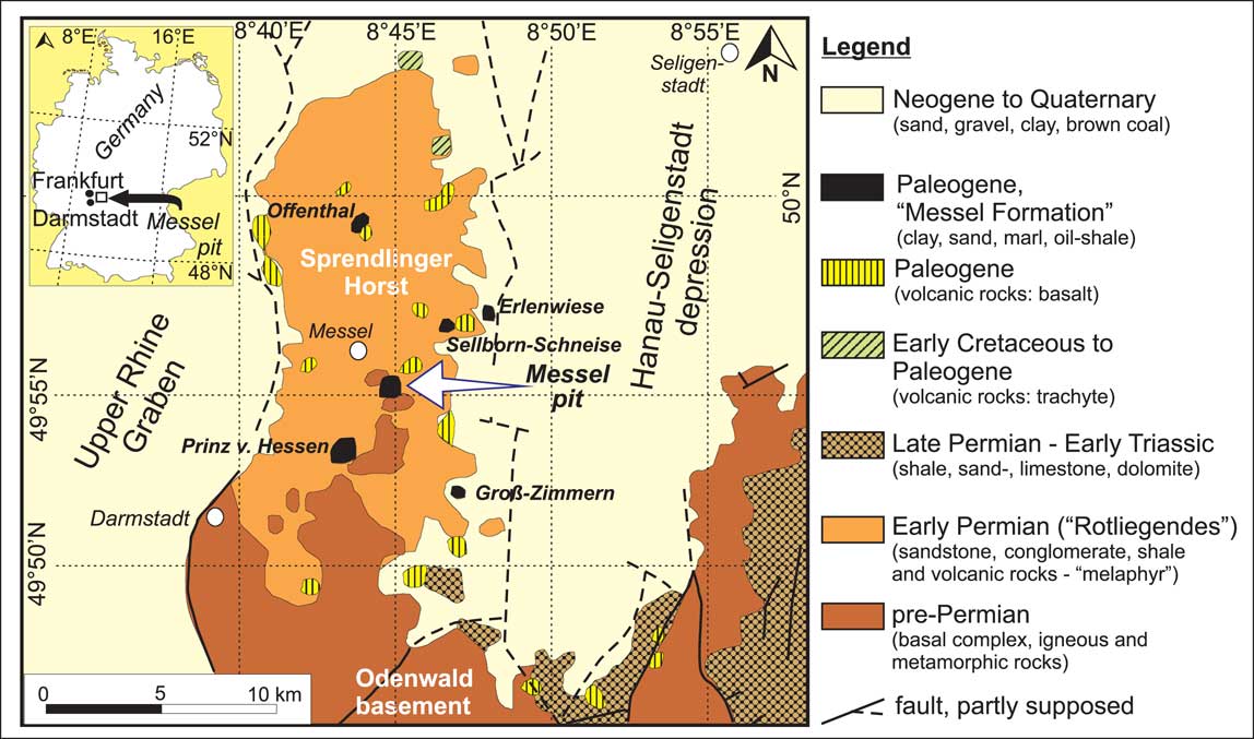
Due to perfect preservation of macrofossils, the lacustrine succession at Messel represents the best known of a series of isolated Paleogene deposits on the Sprendlinger Horst, the northern extension of the Hercynian Odenwald basement in southwest Germany (Fig. 1). About half a dozen isolated basins of limited extent developed (e.g., Felder et al. Reference Felder, Harms and Liebig2001; Hottenrott Reference Hottenrott2002; Schumacher Reference Schumacher2002; Derer et al. Reference Derer, Schumacher and Schäfer2005; Hinsken et al. Reference Hinsken, Ustaszewski and Wetzel2007), most likely within the context of initial crustal weakness that finally led to the formation of the Upper Rhine Graben as part of the Cenozoic Central European rift system (Hinsken et al. Reference Hinsken, Ustaszewski and Wetzel2007). It has been proven by scientific drilling and geophysical studies that most of these deposits (Fig. 1) are primarily infilling of maar-type volcanic structures piercing through Permian and Lower Triassic host rocks (e.g., Harms et al. Reference Harms, Aderhold, Hoffmann, Nix and Rosenberg1999; Jacoby et al. Reference Jacoby, Wallner and Smilde2000; Felder et al. Reference Felder, Harms and Liebig2001; Felder and Harms Reference Felder and Harms2004). A phreatomagmatic origin for Messel has been proven by a research core from the center of the structure (Lorenz Reference Lorenz2000; Schulz et al. Reference Schulz, Harms and Felder2002; Harms et al. Reference Harms, Nix and Felder2003; Felder and Harms Reference Felder and Harms2004).
Simplified geological situation of the Sprendlinger Horst (modified after Harms et al. Reference Harms, Aderhold, Hoffmann, Nix and Rosenberg1999; Lenz et al. Reference Lenz, Wilde and Riegel2017).

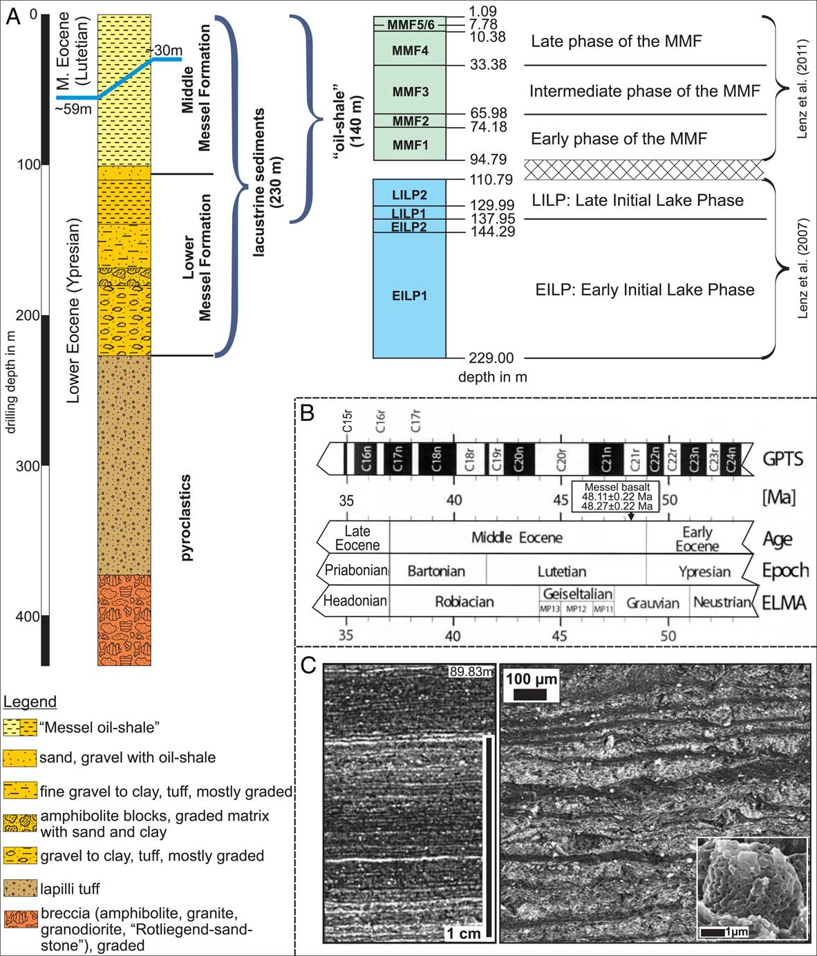
The 229-m-thick lacustrine filling of the maar lake is in its lower part composed of 90 m of clastic sediments of the Lower Messel Formation (LMF), which were deposited during the holomictic stage of the lake (Fig. 2A). According to revised 40Ar/39Ar dating of a basaltic clast from the top of the volcanoclastic material below the lacustrine succession, maar formation started in the early Eocene between 48.27 and 48.11 Ma with a 2-sigma uncertainty of ±0.22 Ma (Lenz et al. Reference Lenz, Wilde, Mertz and Riegel2015; Fig. 2B). The intermittent deposition of laminated bituminous claystones in the upper part of the LMF between 139 and 110 m core depth characterizes the transition to meromictic conditions. The LMF is terminated by an event bed of redeposited blocks of oil shale, oil shale debris, and clay (Felder and Harms Reference Felder and Harms2004), which occurs between 110 and 94 m in the core and can be traced across the entire deposit. The succeeding Middle Messel Formation (MMF) in the upper 94 m is characterized by the classical fossiliferous finely laminated oil shale (Fig. 2A). The fine light and dark lamination (Fig. 2C) was caused by annual algal blooms of the coccal green alga Tetraedron minimum (Goth Reference Goth1990; Lenz et al. Reference Lenz, Wilde, Mertz and Riegel2015). Therefore, an annual varve-like stratification of the oil shale is indicated (Irion Reference Irion1977; Goth Reference Goth1990; Lenz et al. Reference Lenz, Wilde, Riegel and Harms2010), which allowed the establishment of a detailed age model for the deposition of the MMF. Based on varve thickness measurements and continuous sedimentation, a sedimentation rate between 0.10 and 0.15 mm/yr, corresponding to an average rate of 0.14 mm/yr, was calculated (El Bay et al. Reference El Bay, Jacoby and Wallner2001; Schulz et al. Reference Schulz, Harms and Felder2002; Lenz et al. Reference Lenz, Wilde, Riegel and Harms2010), and a deposition time of 640 Kyr for the MMF was determined. Cyclic variations in the pollen rain, which were used for astronomical dating of the MMF, indicate an age between 47.41 and 48.05 or between 47.61 and 48.25 Ma (Lenz et al. Reference Lenz, Wilde, Mertz and Riegel2015). Taking the revised 40Ar/39Ar age for the initial phreatomagmatic explosion(s) into account, a total deposition time for the LMF and the MMF between 700 and 900 Kyr can be estimated (Lenz et al. Reference Lenz, Wilde, Mertz and Riegel2015).
A, Generalized section of core Messel 2001 (after Felder and Harms Reference Felder and Harms2004) showing the subdivision of the lacustrine succession of the maar lake of Messel in 10 different vegetation phases (based on analyses of Lenz et al. Reference Lenz, Wilde and Riegel2007, Reference Lenz, Wilde and Riegel2011). The Ypresian/Lutetian boundary is between 30 and 59 m core depth (see Lenz et al. Reference Lenz, Wilde, Mertz and Riegel2015). EILP, early initial lake phase; LILP, late initial lake phase. B, Stratigraphic position of the Lower and Middle Messel Formation (MMF), including comparison of the Messel Formation related to the magnetostratigraphic (GPTS, global polarity timescale) and biochronologic (ELMA, European land mammal age) timescales; after Mertz and Renne (Reference Mertz and Renne2005); the age of the Messel basalt is taken from Lenz et al. (Reference Lenz, Wilde, Mertz and Riegel2015). C, Laminated oil shale of the Middle Messel Formation showing an annual stratification of alternating light and dark layers. The light, organic-rich layers are characterized by a predominance of remains of the green alga Tetraedron minimum. The detail in the lower right corner presents an individual cell case of T. minimum, showing the typical reticulate sculpture.

Nevertheless, the total time of lake sedimentation is uncertain, because little is known about the Upper Messel Formation (UMF) at the top of the succession, which has been removed by mining activity. According to Matthess (Reference Matthess1956), the UMF consisted of clays and intercalated lignite, probably representing the silting-up phase of Lake Messel.
Methods
Sporomorph Analysis and the Separation of the Lacustrine Succession
The present study is primarily based on the published data of 114 samples from the LMF (Lenz et al. Reference Lenz, Wilde and Riegel2007) and 468 samples from the MMF (Lenz et al. Reference Lenz, Wilde and Riegel2011). The number of studied samples has been increased recently by counting 50 additional samples from the MMF (Lenz et al. Reference Lenz, Wilde and Riegel2017) and 48 additional samples from the oil shale–free part of the LMF below 140 m core depth. Therefore, a total of 680 samples was available for diversity analyses.
In the oil shale–free part of the LMF, samples were selected on the basis of lithology, especially including dark sediments in which a sufficient content of organic material could be expected. In the upper part of the LMF above 139 m core depth, in which the oil shale dominates (Fig. 2A), 1-cm-thick slices of oil shale, covering ca. 71 yr on average, were studied in 40 cm intervals (Lenz et al. Reference Lenz, Wilde and Riegel2007). In the MMF above 94 m, the sampling intervals were reduced to 20 cm (Lenz et al. Reference Lenz, Wilde and Riegel2011) and in parts to 10 cm (Lenz et al. Reference Lenz, Wilde and Riegel2017).
Based on numerical treatment of palynological data by two-way indicator species analysis four vegetation phases have been distinguished during the LMF (Lenz et al. Reference Lenz, Wilde and Riegel2007; Fig. 2A), the “early initial lake phases 1 and 2” (EILP1, EILP2) and the “late initial lake phases 1 and 2” (LILP1, LILP2), that in total document the recolonization of the volcanically disturbed site by plants. The pollen diagram of the MMF was subdivided into six zones (Lenz et al. Reference Lenz, Wilde and Riegel2011) by using optimal splitting by information content (Bennett Reference Bennett2005), a method well suited for a robust zonation in relatively uniform pollen spectra (Rull Reference Rull2003; Bennett Reference Bennett2005). These six zones (MMF1 to MMF6) represent different steps during the evolution of the climax vegetation at Messel (Fig. 2A). Therefore, 10 phases, which were identified by objective numerical methods, can be distinguished during the development of the vegetation (Fig. 2A). Here, calculations of plant diversity are presented for all samples from these 10 phases. The part between 110.79 and 94.79m core depth is not included in our biodiversity estimates, because this part of the core is characterized by redeposited sediments (Felder and Harms Reference Felder and Harms2004).
About 300 palynomorphs were counted per sample. Nevertheless, between 10% and 15% of the total assemblage (Lenz et al. Reference Lenz, Wilde and Riegel2007, Reference Lenz, Wilde and Riegel2011, Reference Lenz, Wilde and Riegel2017) could not be determined and was recorded as “Varia.” Therefore, 220 to 280 individual counts have been used per sample for diversity analyses. The raw data are included in the Supplementary Material.
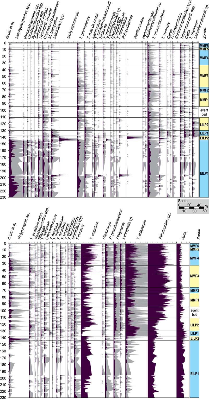
The percentage values of the 54 most important palynomorphs or groups of palynomorphs with more than 1% in at least one sample are presented in the new pollen diagram (Fig. 3, Supplementary Table 1), which includes the counts of Lenz et al. (Reference Lenz, Wilde and Riegel2007, Reference Lenz, Wilde and Riegel2011), the 98 new samples, and 35 samples taken from the event bed between the LILP2 and phase MMF1. The taxa are arranged according to their score along the first axis of an NMDS gradient analysis to better visualize the differences between the 10 vegetational phases. The pollen diagram was produced using PanPlot v. 11.04 (Alfred Wegener Institut für Polare und Marine Forschung, PANGEA).
Overall pollen diagram of 715 samples from core Messel 2001 between 1.09 and 229 m depth. The subdivision of the diagram is based on Lenz et al. (Reference Lenz, Wilde and Riegel2007, Reference Lenz, Wilde and Riegel2011). For statistical analyses, 680 samples from early initial lake phase (EILP), late initial lake phase (LILP), and Middle Messel Formation (MMF) zones were used. The 35 samples from the event bed were excluded because of redeposition.

Paleoclimatic and Paleoecologic Interpretation
Fauna and flora had reached an evolutionary state already similar to today in the Paleogene. This allows the reconstruction of the vegetation and the climatic requirements of its components by relating the fossil palynomorph taxa to modern analogues, which were identified mainly by Thiele-Pfeiffer (Reference Thiele-Pfeiffer1988) and are here presented in Supplementary Table 1. Our interpretation is based on the assumption that the climatic requirements of individual taxa have not changed substantially since the Paleogene. Nevertheless, since most Eocene pollen can only be assigned to the family level, which is of limited value in determining paleoclimatological status, we used abundance changes of palynomorphs within the lacustrine succession to extract information about relative climate changes.
The oil shale of the MMF is particularly well-suited for analyses of relative climate changes, because facies conditions and sedimentation rate remained stable throughout the time interval of 640 Kyr. The pollen assemblages probably were not influenced by changes in taphonomic conditions within the lake or in the surrounding catchment area. Therefore, we concluded that the frequency distribution of palynomorphs reflects shifts in the composition of the paratropical climax vegetation, which were essentially induced by climate variability. The high-resolution study of the MMF therefore allowed the identification of relative climate changes on millennial timescales.
In contrast, the deposits of the older LMF with alternating breccias, tuffs, and layers of sand and clay allowed only rough estimates on climate changes and variability, because the time of deposition cannot accurately be identified. Therefore, the LMF has been excluded from our time-series analyses. Nevertheless, the palynomorphs of the LMF could be used to reconstruct the vegetation during the recolonization of the disturbed area by comparison with modern analogues of the parent plants.
Non-metric Multidimensional Scaling
To illustrate compositional differences and ecological trends between the different vegetation phases in Messel, NMDS (Shepard Reference Shepard1962a, Reference Shepardb; Kruskal Reference Kruskal1964) was performed for the entire data set using the software PAST (Hammer et al. Reference Hammer, Harper and Ryan2001). This ordination method was chosen as the appropriate multivariate model, because NMDS is the most robust unconstrained ordination method in ecology (Minchin Reference Minchin1987) and has been successfully applied to palynological data in previous studies (e.g., Oswald et al. Reference Oswald, Faison, Foster, Doughty, Hall and Hansen2007; Jardine and Harrington Reference Jardine and Harrington2008; Mander et al. Reference Mander, Kürschner and McElwain2010; Ghilardi and O’Connell Reference Ghilardi and O’Connell2013; Broothaerts et al. Reference Broothaerts, Verstraeten, Kasse, Bohncke, Notebaert and Vandenberghe2014). NMDS avoids the assumption of a linear response model (like principal components analysis) or a unimodal response model (like correspondence analysis) between the palynomorph taxa and the underlying environmental gradients, and it also avoids the requirement of normality of data.
For NMDS we used the Bray-Curtis dissimilarity and the Wisconsin double standardized raw data values (Bray and Curtis Reference Bray and Curtis1957; Gauch and Scruggs Reference Gauch and Scruggs1979; Oksanen Reference Oksanen2007). Wisconsin standardization scales the abundance of each taxon to its maximum value and represents the abundance of each taxon by its proportion in the sample (Mander et al. Reference Mander, Kürschner and McElwain2010). This equalizes the effects of rare and abundant taxa and removes the influence of sample size on the analysis (Van Tongeren Reference Van Tongeren1995; Jardine and Harrington Reference Jardine and Harrington2008).
All taxa that occur in at least one sample as more than 1% were included in the analysis. Nevertheless, to avoid possible sources of error that can have an impact on the results, the data set was simplified for NMDS. Some of the palynomorph taxa (families, genera, or individual species) were lumped to minimize problems in the identification to “species” level, because of preservation of some pollen grains or very small morphological differences between some species (e.g., species of the juglandaceous genus Plicatopollis; Lenz et al. Reference Lenz, Wilde and Riegel2007, Reference Lenz, Wilde and Riegel2011). Therefore, for multivariate analysis, the different taxa were assigned to 54 “variables” (Supplementary Table 1).
Biodiversity Analysis
To estimate changes in taxonomic diversity between single samples and between the 10 vegetation phases, several methods were used. We focus on two important biodiversity parameters: species richness and evenness.
Richness is defined as the number of taxa within an ecosystem, which is here calculated as the total number of palynological taxa within a sample (Keen et al. Reference Keen, Gosling, Hanke, Miller, Montoya, Valencia and Williams2014). However, species richness can neither be accurately measured nor directly estimated by observation, because the observed number of species is a downward-biased estimator for the complete species richness in an assemblage (Gotelli and Colwell Reference Gotelli and Colwell2010). Several methods have been developed to correct this bias. With the Bernoulli product model as a new tool for biodiversity analysis as provided by Colwell et al. (Reference Colwell, Chao, Gotelli, Lin, Mao, Chazdon and Longino2012) and Colwell (Reference Colwell2013), it is now possible not only to calculate species richness by a combination of interpolation and extrapolation within a single sample or a sequence of samples, but also to present an error estimation for such calculations with the indication of 95% confidence intervals for interpolated and extrapolated richness estimates. This allows rigorous statistical comparison of biodiversity calculations of samples or successions. Nevertheless, palynological data have additional biases such as variable taxonomic resolution and regular variation in pollen precipitation, with the latter influenced by random effects such as pollen production, dispersal, and deposition (Prentice Reference Prentice1980). Therefore, diversity estimates using palynomorphs are always an underestimate, and the corrections of palynological diversity by the Bernoulli product model are not entirely accurate. We applied the software EstimatesS v. 9.1.0 (Colwell Reference Colwell2013) for calculation and construction of rarefaction curves with interpolated and extrapolated data.
Plant richness can be measured at different scales, for which mainly three terms are used—namely, alpha, beta, and gamma diversity (Whittaker Reference Whittaker1972). The definitions of these terms are originally based on the spatial comparison of diversity in different areas or regions. However, we use these terms to describe the temporal comparison of diversity changes within the succession at Messel.
Alpha diversity is local richness or diversity and is normally estimated within a defined area such as a vegetation quadrat or forest (Birks et al. Reference Birks, Felde, Bjune, Grytnes, Seppä and Giesecke2016). For Messel, we use alpha diversity as a measure for palynomorph richness or diversity within a single sample representing diversity within the plant community at a specific time during the deposition of lacustrine sediments at Messel. Gamma diversity, normally the total diversity estimated or measured for a group of localities in an area (Birks et al. Reference Birks, Felde, Bjune, Grytnes, Seppä and Giesecke2016), is used as a measure of richness within each of the 10 vegetational phases at Messel. Beta diversity links alpha and gamma and is a measure of the difference in species composition between two or more areas or samples (Whittaker Reference Whittaker1972; Ellison Reference Ellison2010; Beck et al. Reference Beck, Holloway and Schwanghart2013; Birks et al. Reference Birks, Felde, Bjune, Grytnes, Seppä and Giesecke2016).
The richness estimations are based on 220 to 280 individual grains per sample. This is a relatively small number and the detection probability for rare taxa is therefore low. Weng et al. (Reference Weng, Hooghiemstra and Duivenvoorden2006) calculated that within a sample, a pollen count of 300 grains is usually enough to detect taxa with a frequency of >1%, but taxa with a frequency <1% may only be detected by chance. Therefore, the calculation of the number of palynological species within a single sample (alpha diversity) in the succession at Messel is an underestimate of the possible number of species. However, this applies to all samples in the same way. Therefore, it can be assumed that at least relative changes of alpha diversity have been reliably detected. On the other hand, for the calculation of gamma diversity, it can be assumed that due to the high number of analyzed samples in each of the 10 vegetational phases and the large total number of counted palynomorphs (e.g., 164 samples and more than 40,000 individual pollen and spores in phase MMF4), most of the very rare taxa are recognized in at least some of the samples.
To examine within-sample diversity and for the calculation of alpha diversity, individual rarefaction was applied using PAST (Hammer et al. Reference Hammer, Harper and Ryan2001). In this way, the species richness of all samples within each of the 10 phases at the same number of counted species (200 sporomorph grains per sample) were compared.
For the calculation of gamma diversity in each of the 10 vegetational phases, the sample-based abundance data set was converted to a sample-based incidence data set to calculate incidence-based extrapolation curves using the Bernoulli product model following Colwell et al. (Reference Colwell, Chao, Gotelli, Lin, Mao, Chazdon and Longino2012). Because of differences in the total number of counted individuals per sample, the sample-based rarefaction curves and their confidence intervals are replotted against an x-axis of individual abundance as suggested by Gotelli and Colwell (Reference Gotelli and Colwell2010), allowing for a sound comparison between assemblages of differing sample sizes.
Rarefaction curves of gamma diversity were calculated without replacement and were extrapolated mainly to twice the number of collected samples. Extrapolation to about three times the original sample number was performed only for the three vegetational phases with low numbers of samples: EILP2, LILP1, and MMF5. To get smooth rarefaction curves, 100 sample-order randomizations were used.
Ecologists have developed several ways to calculate beta diversity based on presence/absence data (Wilson and Shmida Reference Wilson and Shmida1984; Magurran Reference Magurran1988; Koleff et al. Reference Koleff, Gaston and Lennon2003). While alpha and gamma diversities can be directly measured or estimated, beta diversity is derived from alpha and gamma diversities, but there is no consensus about derivation and interpretation of this quantity (Ellison Reference Ellison2010; Birks et al. Reference Birks, Felde, Bjune, Grytnes, Seppä and Giesecke2016). Here we adapt Whittaker’s (Reference Whittaker1960, Reference Whittaker1972) original suggestion, which is most frequently employed in ecological studies (Koleff et al. Reference Koleff, Gaston and Lennon2003). Hence, beta diversity is a measure of the proportion by which the species richness of a region exceeds the average richness of a single locality within that region (Koleff et al. Reference Koleff, Gaston and Lennon2003). Therefore, for the 10 vegetational phases at Messel, beta diversity is calculated by the total number of species within a vegetational phase divided by the average species number within a sample of the specific phase using PAST (Hammer et al. Reference Hammer, Harper and Ryan2001). High beta diversity indicates large fluctuations and changes in taxonomic composition of palynomorphs from sample to sample.
Evenness is another important measure of biodiversity, described in our study as the distribution of pollen taxa within a pollen assemblage (Birks et al. Reference Birks, Felde, Bjune, Grytnes, Seppä and Giesecke2016). A sample with a dominant taxon, characterized by a high number of pollen grains of the same type, has a low evenness, whereas a sample without dominant taxa, indicated by equally distributed taxa, represents a high evenness (Smith and Wilson Reference Smith and Wilson1996). However, it must be kept in mind that plants produce varying amounts of pollen that are distributed differentially. Therefore, one must be cautious when linking evenness within a pollen assemblage to evenness of the parent vegetation when interpreting diversity of vegetation (Keen et al. Reference Keen, Gosling, Hanke, Miller, Montoya, Valencia and Williams2014).
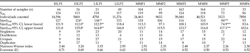
We calculate evenness (E) using the formula provided by Keen et al. (Reference Keen, Gosling, Hanke, Miller, Montoya, Valencia and Williams2014). Two variables are required: (1) richness (R) and (2) the Shannon-Wiener index (H). With the formula E=H/ln(R), an evenness value is produced, which varies between 0 (low evenness) and 1 (high evenness). For R we used the richness estimations within 100 samples provided by Colwell et al. (Reference Colwell, Chao, Gotelli, Lin, Mao, Chazdon and Longino2012; Table 1). If evenness is the same for samples, differences in richness will correspond to differences in diversity, and if richness is the same, then differences in evenness will correspond to differences in diversity (Kindt and Coe Reference Kindt and Coe2005).
Estimations of richness and evenness using sample-based incidence data for the 10 vegetation phases of the Lower Messel Formation (EILP, LILP) and Middle Messel Formation (MMF). Sobs, actual number of taxa within the samples; S(est)100, expected number of species in 100 samples using the Bernoulli product model (Colwell et al. Reference Colwell, Chao, Gotelli, Lin, Mao, Chazdon and Longino2012); S(est)100 95% CI, lower and upper bounds of 95% confidence interval for S(est); *S(est) and S(est) 95% CI in 75 samples; **S(est) and S(est) 95% CI in 63 samples; ***S(est) and S(est) 95% CI in 39 samples; singletons, no. of species that occur only once in all samples; doubletons, no. of species that occur only twice in all samples; uniques, no. of species that occur in only one sample; duplicates, no. of species that occur in only two samples; E, evenness calculation using the method of Keen et al. (Reference Keen, Gosling, Hanke, Miller, Montoya, Valencia and Williams2014): E=Shannon-Winter index/ln(Sobs).

Time-Series Analysis
For the recognition of persistent cyclic patterns in alpha diversity within 468 samples taken in 20 cm intervals from the MMF between 3.08 and 94.60 m core depth, we applied two independent techniques of spectral analysis (REDFIT procedure and wavelet transform) using PAST (Hammer et al. Reference Hammer, Harper and Ryan2001). To get comparable results, the same samples have been chosen as in the studies of Lenz et al. (Reference Lenz, Wilde and Riegel2011, Reference Lenz, Wilde, Mertz and Riegel2015), in which cyclic changes in the composition of the vegetation have already been recognized. Assuming a constant sediment accumulation rate of 0.14 mm/yr (Lenz et al. Reference Lenz, Wilde, Riegel and Harms2010), the sample interval of 20 cm corresponds to a time interval of about 1400 yr. Therefore, a record of 640 Kyr is represented by the analyzed 91.52-m-long section from the MMF.
The REDFIT procedure of Schulz and Mudelsee (Reference Schulz and Mudelsee, M.2002) is designed to test whether dominant frequencies in the spectrum of a time series are significant against a red-noise background from a first-order autoregressive (AR1) process. For calculation of significant peaks, a Monte Carlo simulation was performed using 1000 random realizations of an AR1 process (Hammer et al. Reference Hammer, Harper and Ryan2001, PAST). To achieve clear and significant peaks, the Welch-type spectral window was applied using two overlapping (50%) segments and an oversampling rate of 3.
Additionally, we used the Morlet wavelet (Morlet Reference Morlet1983; Torrence and Compo Reference Torrence and Compo1998), a continuous wavelet transform, which visualizes a time series in a time–frequency space, allowing identification of the dominant frequency signals and determination of their variation with time (Torrence and Compo Reference Torrence and Compo1998).
Comparison of Compositional and Diversity Changes in the Vegetation
Lenz et al. (Reference Lenz, Wilde and Riegel2011) showed that the taxonomic composition of the palynoflora remained similar throughout the deposition of the MMF. Nevertheless, cyclic fluctuations of different orders in the quantitative composition of the microfloral assemblages were evident. A cluster analysis of the samples between 3.08 and 94.60 m core depth resulted in eight palynomorph assemblages according to their frequency distribution (Lenz et al. Reference Lenz, Wilde and Riegel2011, Reference Lenz, Wilde, Mertz and Riegel2015)
The frequency graphs of these eight clusters were used as a database for time-series analyses, which revealed that the pollen assemblages show frequency fluctuations within the Milankovitch range of eccentricity, obliquity, and precession (Lenz et al. Reference Lenz, Wilde and Riegel2011). Precession-paced vegetation changes with fluctuations in the range between 20 and 24 Kyr became obvious, whereas the short eccentricity signal of 100 Kyr is modulated by the amplitude of the precession signal (Lenz et al. Reference Lenz, Wilde, Mertz and Riegel2015).
The Gaussian band-pass-filtered short eccentricity and precession modulations of the palynomorph clusters were primarily used for an astronomical tuning of the MMF (Lenz et al. Reference Lenz, Wilde, Mertz and Riegel2015), but here we chose the amplitude modulations (AMs; PAST; Hammer et al. Reference Hammer, Harper and Ryan2001) of five of these eight clusters to compare the frequency variations of the pollen clusters, which reflect regular compositional changes of the vegetation at Messel, with the AMs of alpha-diversity variations in the MMF. Additionally, to quantify phase shifts between the AMs of alpha diversity and the AMs of the five palynomorph clusters, phase wheels have been constructed (see also the Supplementary Material).
Results
Lower Messel Formation
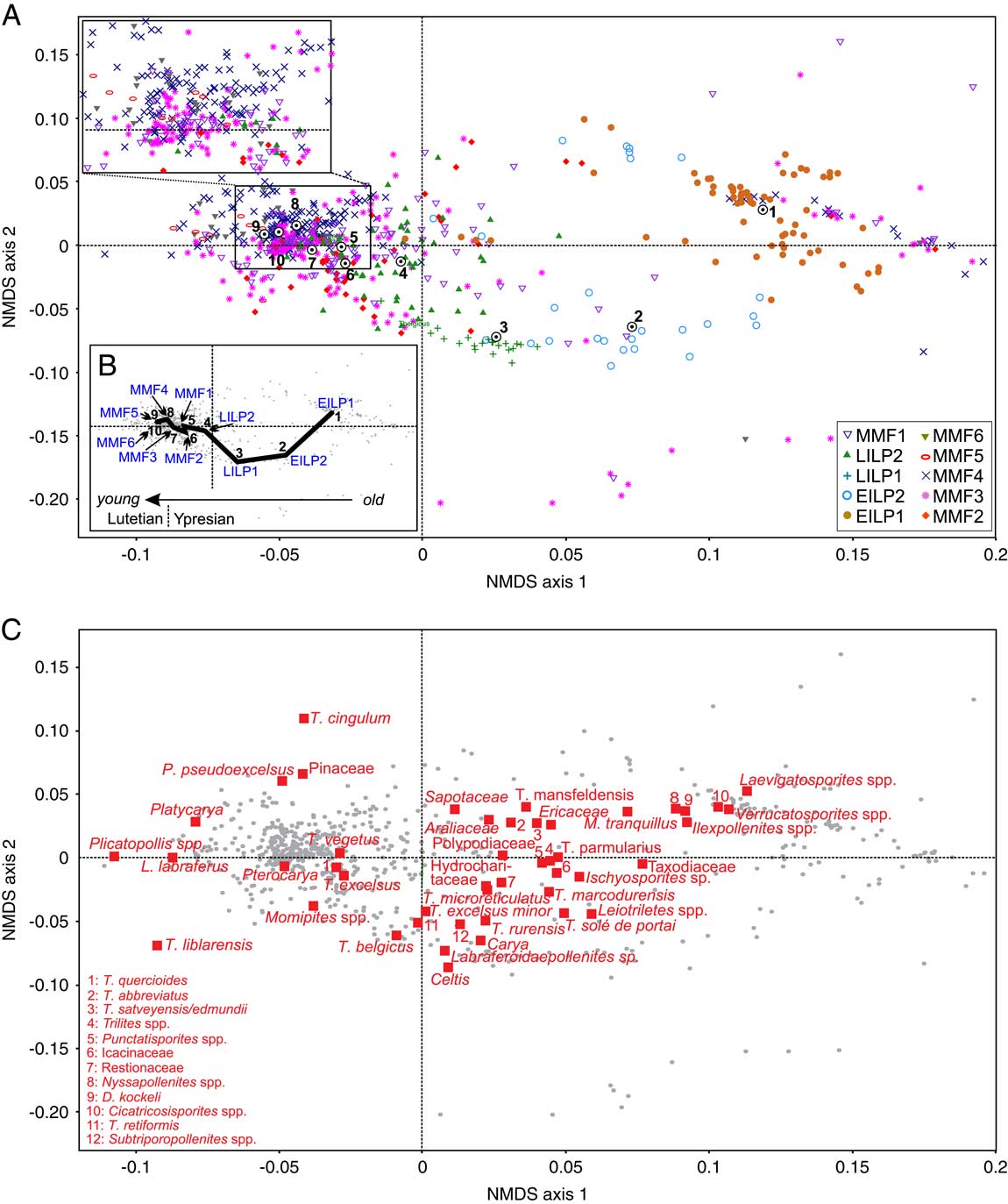
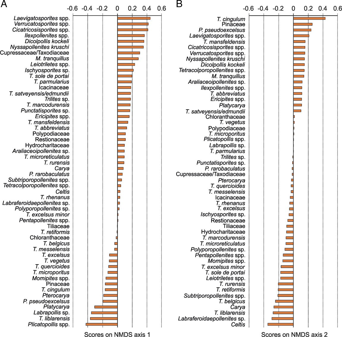
The overall pollen diagram shows that there is a continuous change in the composition of the vegetation during the different phases of the LMF (Fig. 3). This is confirmed by NMDS, because the samples from the early initial lake phase (EILP1, EILP2) group separately in the ordination space on the right end of the NMDS plot (Fig. 4A), indicating a significant difference in composition between the palynomorph assemblages of EILP1 and EILP2 (Fig. 4B). The pollen diagram (Fig. 3) and the NMDS plot of the taxa (Fig. 4C) show that the distribution of different fern spores is the main factor for the separation of EILP1 and EILP2, because Laevigatosporites spp., Verrucatosporites spp., and Cicatricosisporites spp. are among the dominant spores in EILP1, whereas Ischyosporites sp., Leiotriletes spp., and Polypodiaceoisporites spp. and Verrucingulatisporites sp. (both combined as Polypodiaceae) are abundant fern spores in EILP2. Consequently, the dominating fern spores of EILP1 are characterized by higher NMDS scores along axes 1 and 2 than the prevailing spores of EILP2 (Fig. 5).
Non-metric multidimensional scaling (NMDS) of palynological data of 680 samples from the lacustrine succession of the Messel maar lake using the Bray-Curtis dissimilarity and the Wisconsin double standardized raw data values. A, Scatter plot of the first two axes showing the arrangement of samples. The different symbols represent samples from the 10 different vegetation phases. The numbers indicate the median NMDS scores of the different vegetation phases. B, Position of the 10 vegetation phases based on median NMDS scores in the ordination space. The black line indicates a gradual but continuous vegetation change from early initial lake phase 1 (EILP1) to Middle Messel Formation 6 (MMF6). LILP, late initial lake phase. C, Scatter plot of the first two axes showing the arrangement of taxa. The dots represent the different samples (see A).

Scores on (A) non-metric multidimensional scaling (NMDS) axis 1 and (B) NMDS axis 2 for 54 pollen taxa counted over the 10 vegetational phases of Lake Messel.

Furthermore, the pollen diagram reveals that the palynomorph assemblages from the late initial lake phase (LILP1, LILP2) are different compared with those from the EILP (Fig. 3). This is mainly related to the disappearance of most of the fern spores toward the end of the EILP. During the LILP especially, forest plants such as those from the juglandaceous alliance (e.g., Carya, Platycarya, Plicatopollis spp., Labraferoidaepollenites sp.) became dominant (Fig. 3). Additionally, the samples of LILP1 and LILP2 are also slightly separate from each other in the NMDS (Fig. 4A,B), indicating that there are minor differences between the palynomorph assemblages of both phases. Notably, the samples from LILP2 are plotted in the ordination space together with samples from the older phases of the MMF (Fig. 4A), pointing to a similar composition of the vegetation.
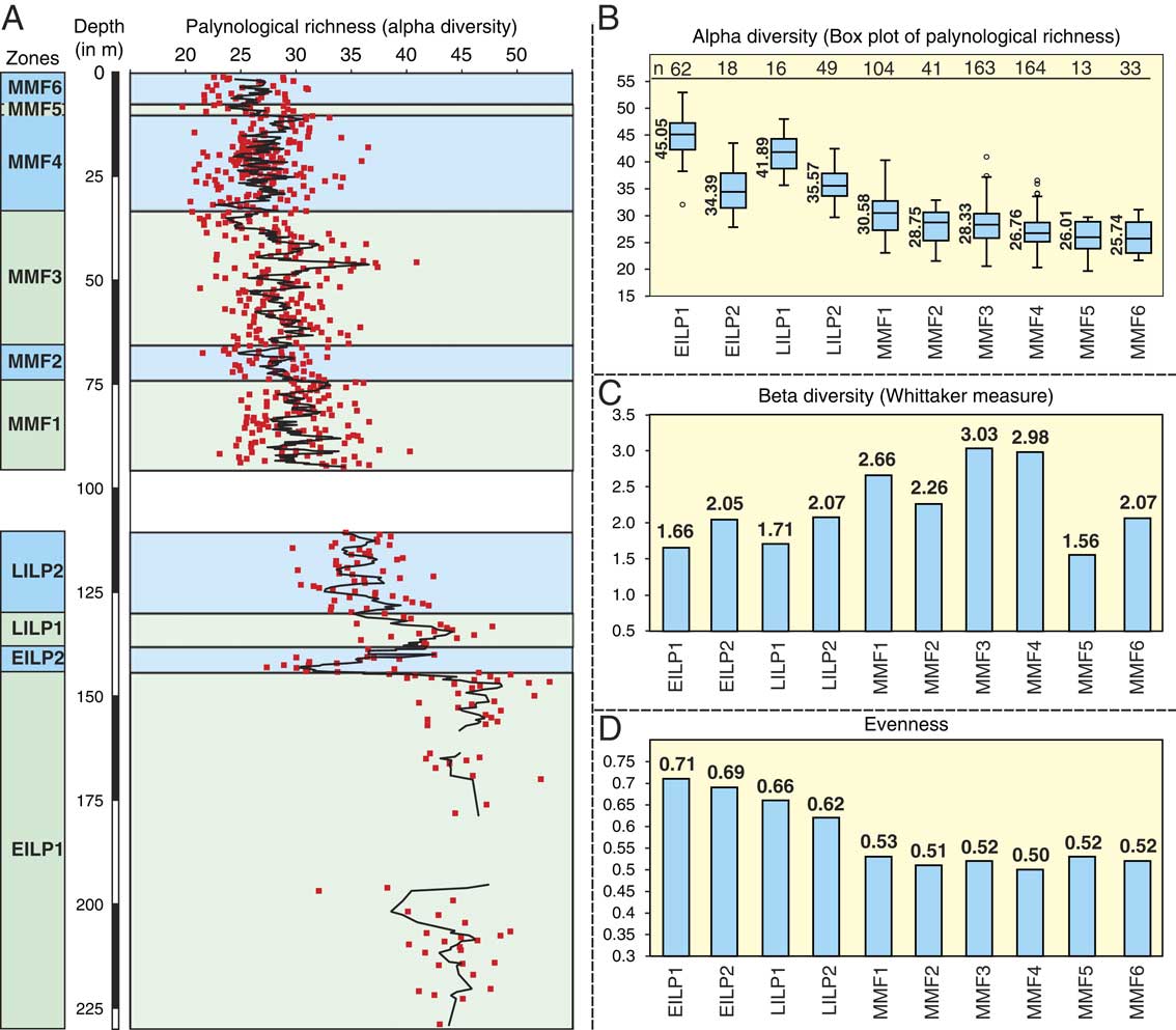
In addition to changes in the composition of the pollen assemblages, there are also obvious changes in alpha and gamma diversity between the four initial lake phases (Figs. 6, 7). The highest alpha diversity for the complete succession at Messel is achieved in EILP1, followed by a significant decrease in EILP2 (Fig. 6A,B). Afterward, alpha diversity increases again in LILP1 (Fig. 6B). In LILP2, the average alpha diversity is still high and exceeds the values of the samples from the following MMF (Fig. 6A,B).
A, Rarefied within-sample richness (alpha diversity) at 200 counted individual palynomorphs for 680 samples from Lake Messel. The black line represents the five-sample moving average. EILP, early initial lake phase; LILP, late initial lake phase; MMF, Middle Messel Formation. B, Box-and-whisker plot of rarefied within-sample richness (alpha diversity) at 200 counted individual palynomorphs for the 10 vegetation phases of Lake Messel. The box represents the 25%–75% quartiles with the median with a horizontal line inside the box. The median values are behind the boxes. The whiskers are drawn from the top of the box up to the largest data value that is less than 1.5 times the box height from the box, and similarly below the box. Outliers are presented with circles. The numbers (n) in the upper line represent the number of samples used for calculating each of the plots. C, Bar chart of beta diversity calculated for the 10 vegetation phases using the measure of Whittaker (Reference Whittaker1960, Reference Whittaker1972): (S/ā ) – 1; S, total number of species in a vegetation phase, ā, average number of species in a sample of the specific vegetation phase. D, Bar chart with evenness values for the 10 vegetation phases. The calculation is based on species richness estimations and the Shannon-Wiener index (see Table 1).

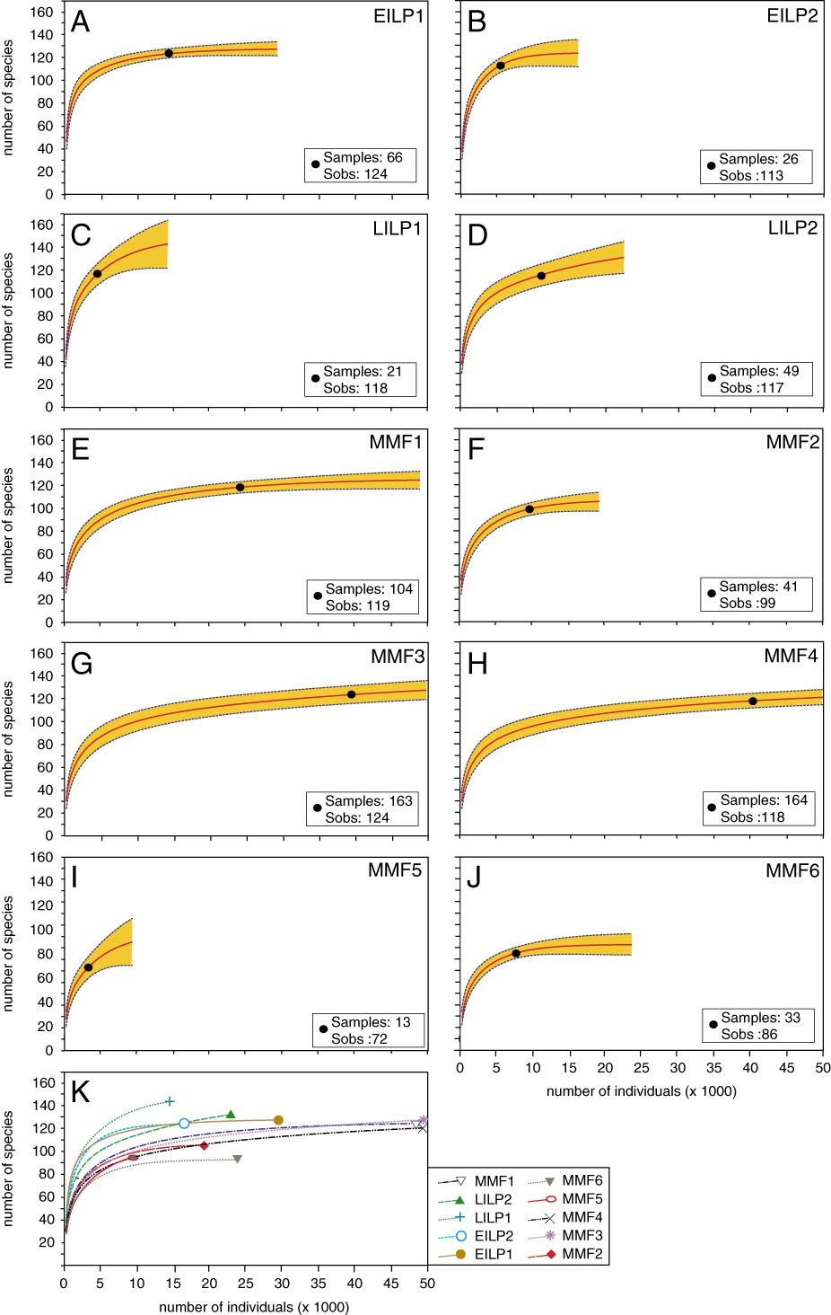
Sample-based interpolation (rarefaction) and extrapolation using the Bernoulli product model (Colwell et al. Reference Colwell, Chao, Gotelli, Lin, Mao, Chazdon and Longino2012) for the 10 vegetation phases of the Lower (LMF) and Middle (MMF) Messel Formation with 95% unconditional confidence intervals: A, early initial lake phase 1 (EILP1), 66 samples; B, EILP2, 26 samples; C, late initial lake phase (LILP1) 1, 21 samples; D, LILP2, 49 samples; E, MMF1, 104 samples; F, MMF2, 41 samples; G, MMF3, 163 samples; H, MMF4, 164 samples; I, MMF5, 13 samples; J, MMF6, 33 samples. K, Comparison of the curves from the 10 lake phases of the LMF and MMF. For clarity, the 95% confidence intervals are omitted. Because of differences in the number of counted individuals per sample, the sample-based rarefaction curves and their confidence intervals are replotted against an x-axis of individual abundance. Sobs, number of observed species.

A slightly different trend can be seen in gamma diversity. Here, the highest diversity is reached in LILP1 (Fig. 7C,K). Gamma diversity increases by ~15% from EILP1 and EILP2 to LILP1. It must be noted that the count of 144 species calculated for LILP1 by the Bernoulli product model of Colwell et al. (Reference Colwell, Chao, Gotelli, Lin, Mao, Chazdon and Longino2012) is based on an extrapolation within only 63 samples from LILP1, while the number of species in EILP1 is based on an extrapolation within 100 samples and in EILP2 within 75 samples (Table 1). Accordingly, a further increase of the number of species in LILP1 can be expected by an extrapolation within a sample number higher than 63, but the Bernoulli product model gives valid results only up to tripling of the original sample size of 21 (Colwell et al. Reference Colwell, Chao, Gotelli, Lin, Mao, Chazdon and Longino2012). Therefore, the graph for LILP1 (Fig. 7C) is not saturated, whereas the two graphs from the early initial lake phase are characterized by the same asymptotic shape of the expected richness curves (Fig. 7A,B). This indicates that a significant increase of the species number in both EILP1 and EILP2 is unlikely, even if a higher number of samples were studied, while the unsaturated graph of LILP1 shows that the maximum expected number of species is far higher than 144. However, the 95% confidence intervals, which describe the range of the possible number of species, overlap somewhat (Fig. 7, Table 1). An increase in gamma diversity from EILP1/EILP2 to LILP1 is therefore indicated but not statistically significant, but this is probably due to the low number of only 21 samples in LILP1 and the extrapolation to a tripling of the sample number, which is accompanied by a relatively high calculation error (Table 1).
In LILP2, the number of expected species for gamma diversity decreases to the same level that is achieved in the early initial lake phase (Table 1, Fig. 7K). Nevertheless, the interpolation/extrapolation graph is not saturated, indicating that the maximum number of species is higher than calculated and probably higher than in EILP1 and EILP2 (Fig. 7D).
Middle Messel Formation
The overall pollen diagram (Fig. 3) shows that a relatively stable thermophilic climax vegetation flourished in the vicinity of Messel during the MMF. The absence of first or last appearances of pollen confirms the stability of the vegetation. The regular frequency fluctuations of most of the palynomorphs are characteristic, indicating the influence of cyclic climate changes (Lenz et al. Reference Lenz, Wilde and Riegel2011). Nevertheless, a gradual change in the palynomorph spectrum of the climax vegetation may be noted, because some elements, such as fern spores of Leiotriletes spp. or pollen of Eucommia (Tricolporopollenites parmularius), decrease from phase MMF1 to MMF6, whereas other elements, such as pollen of Pinaceae or Plicapollis pseudoexcelsus (probably Juglandaceae), increase (Fig. 3).
The gradual change within the palynomorph assemblages from phase MMF1 to phase MMF6 is also recognized by NMDS, because the four youngest phases of the MMF (MMF3 to MMF6) are generally characterized by slightly higher negative NMDS scores on axis 1 (Fig. 4B). Additionally, a general separation of samples from the MMF along NMDS axis 2 is obvious, because most of the samples from the older phases, MMF1 to MMF3, are plotted in the ordination space on the negative side, whereas samples from MMF4 to MMF6 are on the positive side of axis 2 (Fig. 4A). Nevertheless, in the NMDS plot, a series of samples from different phases of the MMF are also plotted in the ordination space of the EILP on the positive side of axis 1 (Fig. 4A).
Compared with the high alpha diversity in the LMF, a significant decline of the species number is obvious in the succeeding phases of the MMF (Fig. 6A). Compared with the highest alpha diversity, which occurs in EILP1, diversity decreases by more than 32% in zone MMF1 (Fig. 6B). In the subsequent zones of the MMF, a further gradual decrease of alpha diversity is recognizable. Therefore, the lowest alpha diversity is reached in the three youngest zones, MMF4 to MMF6 (Fig. 6B).
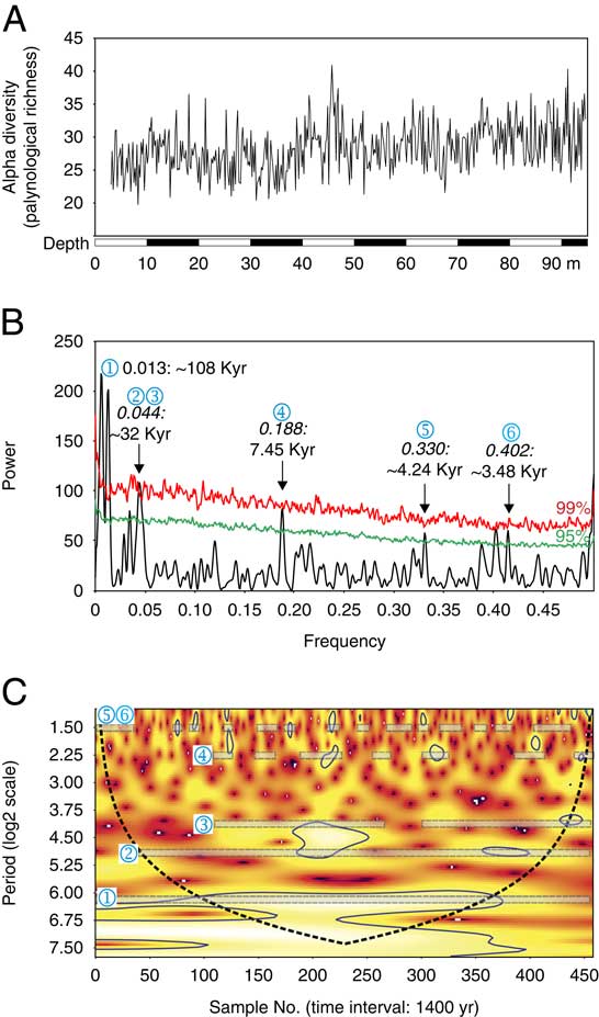
Although the average values in general indicate a low species richness, alpha diversity is subject to strong fluctuations (Figs. 6A and 8A). To test whether these variations are regular, time-series analyses were performed for alpha diversity in the MMF (Fig. 8B,C). The REDFIT analysis identifies highly significant cycles above the confidence limit of 99% with cycle lengths of ca. 108 Kyr, ca. 32 Kyr, ca. 7.5 Kyr, and ca. 3.5 Kyr (Fig. 8B). In addition, a cycle of ca. 4.2 Kyr is above a confidence limit of 95% and can also be considered significant. The additional wavelet analysis shows that the ca. 32 Kyr cycle from the REDFIT analysis is a mixed signal of two cycles varying with periods of ca. 40 Kyr and ca. 24 Kyr (Fig. 8C). In conclusion, the time-series analyses give evidence for a regular change of alpha diversity during the 640-Kyr-long deposition time of the MMF on different timescales.
Time-series analyses of within-sample richness (alpha diversity) at 200 counted individual palynomorphs for 680 samples from core Messel 2001 between 3.08 and 94.60m core depth. A, Time-series data. B, REDFIT analyses of alpha-diversity values. Significant peaks passing the 99% (upper line) or 95% (lower line) Monte Carlo–corrected confidence interval are indicated by frequency and periodicity values. C, Continuous wavelet time–frequency spectra (Morlet wavelets) of alpha-diversity values. To reduce wraparound effects, the time series are padded with zeros. Therefore, the cone of influence indicates the region where boundary effects are present. Bold contours correspond to power that is significant at 95% confidence level. Significant periods are marked by numbers. The numbers point to the respective significant cycles of the REDFIT periodogram.

In phases MMF1 to MMF4, the estimated gamma diversity within 100 samples is between 106 and 118 species (Table 1). Therefore, compared with LILP2, the species number decreases by 11% to 20%, and compared with the highly diverse LILP1, by 18% to 26%. Even if the 95% confidence intervals are taken into account, the decline compared with LILP1 is statistically significant.
The vegetation phases MMF1 to MMF4 show an asymptotic course of rarefaction and extrapolation graphs (Fig. 7). Therefore, the calculated number of species is a robust estimate, which is probably due to the high number of samples, for example, more than 160 in phases MMF3 and MMF4. When the species richness of the four phases is compared, a difference is not recognizable, indicating that gamma diversity is the same (Fig. 7K).
A further decrease in gamma diversity is recorded in the following two phases: MMF5 (96 species) and MMF6 (93 species) from the upper part of the lacustrine succession (Table 1). However, it must be considered that the number of samples within phase MMF5 (13) is very low compared with the other vegetation phases, and the expected number of species could only be extrapolated for 39 samples. Thus, the interpolation/extrapolation graph of species richness is not saturated, and the potential calculation error is relatively high (Fig. 7I). The possible number of species in this zone may therefore be significantly higher (Table 1). Accordingly, when the graph of phase MMF5 is compared with the graphs of phases MMF1 to MMF4, a difference in species richness is not obvious (Fig. 7K).
In contrast, the decrease of species richness by 35% in phase MMF6 compared with LILP1 and by ~17% compared with phases MMF1 to MMF4 is significant (Table 1), because the rarefaction and extrapolation graph is already well saturated (Fig. 7J). The comparison of all graphs also shows the significant decline of the species number in phase MMF6 (Fig. 7K).
Compared with the low alpha and gamma diversities, zones MMF1 to MMF4 are characterized by high values for beta diversity (Fig. 6C). This points to large fluctuations and taxonomic changes from sample to sample.
The high numbers of singletons and doubletons, indicating the number of species with only one or two individuals within the data set, and the numbers of uniques and duplicates, indicating the number of species which occur in only one or two samples, are striking (Table 1). For example, 36 of 118 observed species occur only one or two times in phase MMF1 and 37 of 118 species occur only in one or two samples of this phase (Table 1). As a consequence, between 20% and 40% of the observed species in the different phases are singletons, doubletons, uniques, or duplicates. This implies that the samples are always dominated by a few taxa. Only EILP1 is characterized by a distinctly lower number of singletons/doubletons (13%) and uniques/duplicates (14%). Consequently, the evenness is highest in EILP1 (0.71; Fig. 6D). Because the other three phases from the initial lake phase are also characterized by relatively high evenness values between 0.62 and 0.69, a significant decline of evenness to values between 0.5 and 0.53 is recorded from the LMF to the MMF (Fig. 6D). This implies that the proportion and dominance of some taxa increased within phases MMF1 to MMF6.
Discussion
The first analysis of all palynological data (including the new samples) from the LMF and MMF using NMDS confirms the changes in floristic composition during the evolution of Lake Messel described for the LMF by Lenz et al. (Reference Lenz, Wilde and Riegel2007) and the MMF by Lenz et al. (Reference Lenz, Wilde and Riegel2011). Therefore, the main focus is now on the results of the diversity analyses and the correlation of changes in composition and diversity in the vegetation.
The Composition and Diversity of the Vegetation during the Lower Messel Formation
The phreatomagmatic eruption(s) that formed the maar structure of Messel led to a destruction and disturbance of an area of considerable extent within the lower Eocene paratropical vegetation. The pollen diagram (Fig. 3) and the NMDS plots of the palynomorph data (Fig. 4) reveal that gradual but significant compositional changes within the vegetation occurred starting from the first recolonization of a herbaceous and shrubby pioneer vegetation until a stable climax vegetation was established.
The LMF shows a clear succession of pollen and spore associations representing the colonization of temporary habitats around the lake with different types of a pioneering vegetation, which indicates different stages during the progressive recolonization of the completely devastated habitat after the phreatomagmatic eruption(s) (Lenz et al. Reference Lenz, Wilde and Riegel2007). This is illustrated by an obvious difference between the palynomorph assemblages from EILP1 and EILP2 (Fig. 4A).
An important factor in this context is the speed of the recolonization of the crater area. If the times for recolonization and reforestation in subtropical to tropical regions after disturbance of the habitat, for example, by fire, agriculture, or deforestation, are considered (e.g., Keenan et al. Reference Keenan, Lamb, Wolding, Irvine and Jensen1997; Engel and Parrotta Reference Engel and Parrotta2001), the regeneration and establishment of understory and woody canopy species proceeds within a few years or decades. In fact, recolonization depends on the degree of degradation, proximity to the native forest seedbank, the degree of topsoil loss, and soil fertility (Parrotta Reference Parrotta1995; Keenan et al Reference Keenan, Lamb, Wolding, Irvine and Jensen1997; Lamb et al. Reference Lamb, Erskine and Parotta2005). Nevertheless, a recolonization of the devastated area at Messel by the establishment of an initial forest vegetation within some decades is probable, because a short time span for recolonization coincides with estimates of a rapid deposition for the sediments of the EILP1 and EILP2 in the lower 90 m of the Messel 2001 core. In contrast to the oil shales of the LMF and MMF, which allow for an exact age model due to the annual varve-like stratification (Lenz et al. Reference Lenz, Wilde, Mertz and Riegel2015), a robust chronostratigraphic model cannot be provided, because clastic sediments and intercalations indicating frequent mass movements do not allow calculation of the rate of deposition here. However, due to instability of the crater wall, the sediments have presumably been deposited very quickly in a few tens or hundreds of years (Pirrung et al. Reference Pirrung, Fischer, Büchel, Gaupp, Lutz and Neuffer2003; Lenz et al. Reference Lenz, Wilde, Mertz and Riegel2015). As a result, a centimeter-sized sample of clastic material from the LMF most probably represents a much shorter time span than a centimeter-sized sample from the oil shale.
The regional paratropical climax vegetation, which was distributed in the area before maar formation, still persisted in the hinterland of Lake Messel during the EILP and had reoccupied the area completely at a time representing the boundary between the LMF and MMF (Lenz et al. Reference Lenz, Wilde and Riegel2007). Pollen of the paratropical rain forest therefore never disappeared completely. Especially in the EILP, both the local pioneering vegetation and the surrounding regional paratropical rain forest contributed to the pollen record in the maar lake. Therefore, a high amount of anemophilous pollen from the rain forest in the hinterland is included in the samples of the EILP that, together with the pollen rain of the local pioneering vegetation, cause the high alpha and gamma diversity in EILP1 and EILP2 (Figs. 6, 7).
Toward the end of the EILP, palynomorphs of the initial pioneering vegetation, such as most of the ferns, disappear almost entirely. This is accompanied by a drop in alpha diversity (Fig. 6A,B) and reflects the change from a purely pioneering vegetation to a thermophilic forest successively invading the area around the crater as well as the lake margin. The thermophilic forest reached a climax state in LILP2, as indicated by a strong increase of forest elements (Fig. 3), such as Fagaceae (Tricolporopollenites cingulum) and Juglandaceae (Plicatopollis spp.).
The diversity still increases in LILP1, as rare pollen of entomophilous taxa start to appear (Figs. 6A,B). This is particularly reflected by the extremely high numbers of singletons, doubletons, uniques, and duplicates that occur in LILP1 and LILP2 (Table 1). LILP1 is characterized by the highest palynomorph gamma diversity in the complete record (Fig. 7), because it combines the last elements of the pioneering vegetation with the full spectrum of the thermophilic forest. With the final disappearance of pioneering elements, the diversity of the pollen assemblage therefore decreases slightly in LILP2.
Samples from the LMF are plotted on the positive side of NMDS axis 1 in the ordination space (Fig. 4A), because the NMDS scores of the elements of the pioneering vegetation, such as ferns (Laevigatosporites spp., Verrucatosporites spp., Cicatricosisporites spp.) and palms (Dicolpopollis kockeli), and swamp forest elements, such as Cupressaceae (Inaperturopollenites spp.) and Nyssaceae (Nyssapollenites kruschii), are positive (Fig. 5A). In contrast, the dominant elements of the climax vegetation of the MMF in particular have high negative scores. Consequently, negative scores on axis 1 indicate the forested crater area with the establishment of a climax vegetation, while positive scores indicate a devastated landscape that was settled by pioneering elements and first plants that inhabited the lake shore area. Therefore, the scores on axis 1 can be seen as an indicator for the recolonization process in the vicinity of Lake Messel as the main factor controlling the composition of the pollen assemblages.
The Composition and Diversity of the Vegetation during the Middle Messel Formation
During the MMF, a thermophilic climax vegetation typical of inland sites of western and central Europe during the middle Eocene greenhouse climate (Mai Reference Mai1981, Reference Mai1995; Schaarschmidt Reference Schaarschmidt1988; Wilde Reference Wilde1989; Collinson et al. Reference Collinson, Manchester and Wilde2012) flourished in the crater area and its vicinity (Lenz et al. Reference Lenz, Wilde and Riegel2011). In particular, the juglandaceous alliance (Fig. 4B, e.g., Platycarya, Carya, Engelhardia (Momipites spp.), Plicatopollis spp., Subtriporopollenites spp.) appears highly diverse in the pollen assemblages and probably represents the dominant elements in the forest together with the parent plants of T. cingulum (Fagaceae) and Tricolpopollenites liblarensis (Fagaceae or Leguminosae) (Figs. 3 and 4B). The dominance of few elements within the forest vegetation at Messel explains the significant drop of evenness values from the end of LILP2 to the MMF (Fig. 6D).
The NMDS (Fig. 4A) indicates that the climax vegetation during the MMF did not change substantially in qualitative composition, because most of the samples from the MMF are plotted on the negative side of NMDS axis 1. Nevertheless, a gradual trend within the palynomorph assemblages is obvious from phase MMF1 to phase MMF6, because the individual phases are separated (with overlap) along NMDS axes 1 and 2.
The NMDS scores of palynomorph taxa along axis 2 (Fig. 4B) are characterized by high positive values for T. cingulum and pollen of Pinaceae as well as for some fern spore taxa, such as Laevigatosporites spp. or Cicatricosisporites spp. On the other side, Celtispollenites spp. (Ulmaceae), T. liblarensis, and juglandaceous pollen (Labraferoidaepollenites spp., Caryapollenites spp.) have negative scores. The contrast between negative and positive scores of main elements of the paratropical forest, such as T. liblarensis and T. cingulum, suggest that the scores on axis 2 can be seen as an indicator for variations within the forest composition. Compared with the parent plants of T. cingulum (highest positive NMDS score), the plants producing T. liblarensis (negative NMDS score) are considered to be elements of moister habitats (Riegel et al. Reference Riegel, Lenz and Wilde2015). Therefore, axis 2 may reflect the response of the forest vegetation to climate changes, especially changes of humidity and/or precipitation. The pollen of Pinaceae, which are generally regarded as more tolerant to less humid conditions and well-drained soils than most of the plants known as components of the regular Messel forest (e.g., Mai Reference Mai1995), also indicate less humid conditions. On the other side, Carya and in parts Celtis, which are today important elements of forested wetlands, for example, in the southern United States (Tiner Reference Tiner2017), prefer moister habitats. As a consequence, low scores on axis 2 indicate humid climate conditions, and high scores indicate less humid climate conditions during the evolution of Lake Messel. Therefore, the general vegetation change at Messel is related to a gradual change toward noticeably less humid conditions, possibly in combination with a drop in the lake’s water level (Lenz et al. Reference Lenz, Wilde and Riegel2011).
Nevertheless, in the NMDS plot (Fig. 4A), a series of samples from different phases of the MMF are plotted in the ordination space of the EILP on the positive side of axis 1. This proves that the zonal vegetation did not change in general composition from the earliest stages of the lake during its re-advance into the crater area and the establishment of the climax vegetation. The samples from the early initial lake phase at the beginning of the recolonization process are characterized by a high allochthonous pollen input from the surrounding rain forest. Thus, it is obvious that even after the phreatomagmatic explosion(s) that led to the formation of the crater, the paratropical rain forest still persisted in the catchment area of the pollen rain. The differences between samples from the LMF and most of samples from the MMF, which are indicated by the NMDS, are mainly related to the distribution of pioneering elements in the LMF (Fig. 4).
It is striking that the diversity analyses indicate that in the initial lake phase of the LMF, alpha diversity (Fig. 6A,B) and gamma diversity (Fig. 7) are higher than in the subsequent lake phases of the MMF. During the MMF, the climax vegetation, which was finally established in the crater area during the LILP2, did not change substantially in qualitative composition (Lenz et al. Reference Lenz, Wilde and Riegel2011). Therefore, the diversity analyses show that no fundamental changes in biodiversity occurred between the different phases of the MMF. This is especially documented by gamma diversity using the sample-based approach of the Bernoulli product model (Fig. 7).
The diversity decline from the LMF to the MMF can be explained with a nonequilibrium hypothesis introduced by Connell (Reference Connell1978). After disturbance of a community, for example, by the phreatomagmatic explosion(s) at Messel, recolonization starts when propagules such as seeds or spores of a few species germinate in the open space. Provided there is no further disturbance, diversity increases, because more and more species invade the area. When the tropical rain forest gradually reoccupies the devastated area, the canopy is dominated by a few tree species at the beginning, but the understory is composed of entirely different species. This has been described by Eggeling (Reference Eggeling1947) as mixed tropical rain forest, which is different from the succeeding climax forest. With the establishment of a climax vegetation, diversity declines, because the understory is then composed mainly of juveniles of the canopy species. This can be observed today in tropical rain forests of Africa and South America (Eggeling Reference Eggeling1947; Jones Reference Jones1956; Connell Reference Connell1978). Thus, an assemblage of self-replacing species has become established that represents a climax community of lower diversity. In conclusion, the highest diversity can be found in a nonequilibrium intermediate stage at the beginning of a forest succession (Connell Reference Connell1978).
At Messel, a similar succession of diversity changes can be observed. A high alpha diversity and the highest gamma diversity among the palynological assemblages can be recorded for the LILP1, when the recolonization of the crater area by the paratropical rain forest started and the change from a pioneering vegetation to a mixed paratropical rain forest took place (Figs. 6B and 7K). Considering the intermediate disturbance hypotheses of Connell (Reference Connell1978), the subsequent (humid) climax vegetation, which was finally established at the beginning of MMF1 (Fig. 3), is less diverse compared with the mixed paratropical rain forest of LILP2 in relation to alpha and gamma diversity (Figs. 6B and 7K). Therefore, the vegetation became increasingly less rich in species during the MMF, because a regular disturbance of the habitat (which is responsible for a high diversity) did not occur.
Nevertheless, in addition to the overall decline in alpha and gamma diversity, strong fluctuations of alpha diversity are recognizable for the MMF (Fig. 6A). Time-series analyses of alpha diversity (Fig. 8) reveal a regular change in the number of species with significant variations in the Milankovitch range of short eccentricity (ca. 108 Kyr), obliquity (ca. 40 Kyr), and precession (ca. 24 Kyr).
These orbital parameters strongly affect climate on Earth, especially by influencing the distribution and amount of incident solar energy (Zachos et al. Reference Zachos, Pagani, Sloan, Thomas and Billups2001). In particular, orbital precession influences the seasonal distribution of insolation (Merlis et al. Reference Merlis, Schneider, Bordoni and Eisenman2013), and its changes have great influence on the global distribution and amount of precipitation. Additionally, Zachos et al. (Reference Zachos, Mc Carren, Murphy, Röhl and Westerhold2010) could show that the distribution of tropical elements was favored during times of eccentricity minima, because precipitation was less seasonal and more balanced throughout the year. An influence of eccentricity on precipitation was also suggested by Van Dam et al. (Reference Van Dam, Abdul Aziz, Sierra, Hilgen, van den Hoek Ostende, Lourens, Mein, van der Meulen, A.J. and Pelaez-Campomanes2006), who observed that humidity-adapted rodents and insectivores occurred in high proportions in the western Mediterranean over the last 24 Ma during long eccentricity minima. Eccentricity also controls fluctuations in temperature (van Vugt et al. Reference Van Vugt, Langereis and Hilgen2001), with an increase in temperature during eccentricity minima, which may be responsible for a stronger proliferation of tropical elements (Popescu et al. Reference Popescu, Suc and Loutre2006). Therefore, the shifts from eccentricity minima to maxima were accompanied by a change to less humid conditions and slightly lower temperatures.
Therefore, quantitative changes within the composition of the climax vegetation around Messel (Lenz et al. Reference Lenz, Wilde and Riegel2011, Reference Lenz, Wilde, Mertz and Riegel2015) were probably caused by orbitally controlled latitudinal shifts of climate belts during the monsoonal climate as suggested for the Eocene of Messel by Mai (Reference Mai1995) and Grein et al. (Reference Grein, Utescher, Wilde and Roth-Nebelsick2011). Related changes are the intensity of precipitation as well as slight variations of temperature (Lenz et al. Reference Lenz, Wilde and Riegel2011, Reference Lenz, Wilde, Mertz and Riegel2015).
The same orbital control is now observed for the variation of alpha diversity (Figs. 8, 9). This proves that changes in precipitation and temperature were responsible not only for regular changes in the composition of the vegetation, but also for regular changes in plant diversity.
Comparison of precession and eccentricity band-pass-filtered amplitude modulations (AMs) of percentage graphs of five palynomorph clusters from the MMF (taken from Lenz et al. Reference Lenz, Wilde and Riegel2017) with the respective AMs of within-sample richness (alpha diversity). The records are filtered with a band-pass FIR (finite impulse response) filter centered at 0.065 ± 0.005 cycle/1.4 Kyr, corresponding to periods of 20–23.33 Kyr, for precession (A), and a low-pass FIR filter between 0 and 0.014 cycle/1.4 Kyr, corresponding to periods of >100 Kyr for eccentricity (B) using PAST (Hammer et al. Reference Hammer, Harper and Ryan2001). The negative deflections of 5 eccentricity cycles (e1 – e5) and 30 precession cycles (p1 – p30) are indicated. Clusters A, B, C, D are almost in-phase with alpha diversity, whereas cluster E is in antiphase. Phase wheels for (C) eccentricity and (D) precession present the phase angle of every cycle between the palynomorph clusters and alpha diversity. Zero phase on each wheel is set at minimum eccentricity or precession for alpha diversity. Angular distances from zero correspond to the measured phase differences. Negative or positive phase angles represent the timing of proxy minima relative to the zero point. Positive angles on the left side of the wheel represent cycles in advance of the pollen signal compared with the respective cycle from alpha diversity; a negative angle on the right side represents a lag.

To reveal similarities between orbitally controlled changes in the composition of the vegetation and their diversity, the filtered AMs of short eccentricity and precession of the most important pollen clusters in Messel (Lenz et al. Reference Lenz, Wilde and Riegel2011, Reference Lenz, Wilde, Mertz and Riegel2015; Supplementary Material) have been compared with those of the alpha diversity (Fig. 9). It became evident that both the eccentricity and the precession AMs of the Juglandaceae cluster, composed of different species of the genus Plicatopollis, are in antiphase to the AMs of alpha diversity (Fig. 9A,C). This means that the AMs of alpha diversity have their negative deflections at times when Plicatopollis shows eccentricity and precession maxima. On the other hand, the AMs of the other four clusters used here for comparison, namely the Fagaceae cluster and the clusters of the tropical elements, the swamp elements and the aquatic and hydrophilic elements, are in phase with the AMs of the alpha diversity, with small deviations, as reflected by phase wheels (Fig. 9C,D).
The Fagaceae cluster is composed of two main elements in the palynological record T. liblarensis and T. cingulum. The antiphase coupling of this cluster with the juglandaceous cluster clearly shows that the parent plants of T. cingulum and T. liblarensis alternated with the latter in dominance within the paratropical forest vegetation at Messel (Lenz et al. Reference Lenz, Wilde, Mertz and Riegel2015). The cluster of the aquatic and hydrophilous elements includes pollen and spores of Hydrocharitaceae, Nymphaeaceae, various ferns, and lycopods and reflects the vegetation at the edge of the Messel lake (Lenz et al. Reference Lenz, Wilde, Mertz and Riegel2015). The two clusters of tropical and swamp elements are characterized by a heterogeneous composition. Most notable for the first are pollen taxa of subtropical to tropical elements such as Sapotaceae, Mastixiaceae, and engelhardioid Juglandaceae, as well as Cupressaceae and Nyssaceae for the second cluster.
At Messel a higher amount of pollen and spores assigned to thermophilous and wetland taxa, which were combined here in the two clusters of tropical and swamp elements, correspond to an eccentricity minimum configuration (Lenz et al. Reference Lenz, Wilde, Mertz and Riegel2015), indicating a higher mean annual temperature (MAT) and lower seasonality with more balanced rainfall (Popescu et al. Reference Popescu, Suc and Loutre2006; Zachos et al. Reference Zachos, Mc Carren, Murphy, Röhl and Westerhold2010). There is an in-phase coupling of the two clusters of tropical and swamp elements with the two clusters of the aquatic/hydrophilous elements and the Fagaceae, especially T. liblarensis. This shows that the distribution of the vegetation at the edge of the maar lake, as well as the proliferation of those Fagaceae that prefer more humid conditions (T. liblarensis; Riegel et al. Reference Riegel, Lenz and Wilde2015), is maximized during eccentricity minima. Thus, a more balanced intense rainfall throughout the year was also associated with an increased lake level and more extended areas supporting aquatic and hydrophilous plants. The slightly different distribution of T. cingulum, which is indicative for far less humid conditions (Riegel et al. Reference Riegel, Lenz and Wilde2015), within the Fagaceae cluster could explain that the Fagaceae cluster is not in all cases in phase with the other clusters (Fig. 9D).
The antiphase coupling of the AMs of alpha diversity with the Juglandaceae (Plicatopollis) cluster and the in-phase coupling with the other four clusters now clearly show that diversity within the paratropical vegetation at Messel also increased during times of probably higher and more balanced rainfall and slightly higher MAT.
The influence of millennial-scale fluctuations in the sub-Milankovitch range on the composition of the vegetation has also been recognized in a previous study (Lenz et al. Reference Lenz, Wilde and Riegel2017). The significant ca. 7.45 Kyr cycle for alpha diversity matches the ca. 7.4 Kyr cycle of millennial-scale compositional variations within the pollen assemblages during the MMF (Lenz et al. Reference Lenz, Wilde and Riegel2017) and is close to the ca. 6 Kyr Xapsos cycle, which has been identified in reconstructed numbers of sunspots (Xapsos and Burke Reference Xapsos and Burke2009). Solar activity stimulates cloud formation via cosmic rays, and therefore affects precipitation and/or humidity, but can also influence wind intensity and direction due to a feedback mechanism between cosmic rays and cloud formation (Friis-Christensen and Svensmark Reference Friis-Christensen and Svensmark1997), which modifies pollen transport to a specific site (Kern et al. Reference Kern, Harzhauser, Soliman, Piller and Mandic2013). The maar lake at Messel was an ideal trap reflecting the influence of solar activity, as lake levels are particularly sensitive to solar activity variations and related precipitation changes (Yousef Reference Yousef2006; Bruckman and Ramos Reference Bruckman and Ramos2009). The pollen assemblages of the MMF may therefore indicate a significant influence of solar activity on the diversity of the vegetation.
Furthermore, varve analyses of the laminated oil shale from the MMF clearly show an influence of an Eocene ENSO on the environment at Messel, because significant biennial and decadal components of the time series are almost identical to modern variations of ENSO (Lenz et al. Reference Lenz, Wilde, Riegel and Harms2010). Besides these short-term oscillations, long-term centennial- and millennial-scale ENSO variations are also proven for the Quaternary (Moy et al. Reference Moy, Seltzer, Rodbell and Anderson2002; Stott et al. Reference Stott, Poulsen, Lund and Thunell2002; Turney et al. Reference Turney, Kershaw, Clemens, Branch, Moss and Fifield2004) and may have been responsible for changes in the composition of the vegetation at Messel (Lenz et al. Reference Lenz, Wilde and Riegel2017). Notably, a ca. 3.6 Kyr cycle of such changes at Messel (Lenz et al. Reference Lenz, Wilde and Riegel2017) matches the ca. 3.5 Kyr cycle that can be recognized in the alpha-diversity data set (Fig. 8). Similar variations between 2.5 and 4.0 Kyr were recognized for the past 25 Kyr in southern Africa and interpreted in terms of changes in the frequency of wetter and drier periods, which were possibly caused by millennial-scale teleconnections of an ENSO-like character (Holmgren et al. Reference Holmgren, Lee-Thorp, Cooper, Lundblad, Partridge, Scott, Sithaldeen, Siep Talma and Tyson2003). Further millennial-scale fluctuations of ENSO with a periodicity of ca. 3 Kyr were identified by Horikawa and Ito (Reference Horikawa and Ito2004) in Pleistocene shelf successions from Japan. In this respect, also the ca. 4.2 Kyr cycle, which is significant in the alpha-diversity data set (Fig. 8), may therefore be attributed to such an Eocene millennial-scale ENSO.
It cannot unequivocally be decided if the millennial-scale cycles from Messel should be assigned to solar activity or atmosphere–ocean interaction such as ENSO (Lenz et al. Reference Lenz, Wilde and Riegel2017) Therefore, an interaction of both climate-driving mechanisms may have led to climate variability in the sub-Milankovitch range and to related compositional and diversity changes within the Eocene vegetation at Messel.
The influence of precipitation and temperature variations on the pollen assemblages can also explain the relatively high values for beta diversity in the MMF, which are significantly higher than during the initial lake phases of the LMF. High beta diversity points to large fluctuations and taxonomic changes within the pollen assemblages, which are probably due to the influence of orbitally controlled climate variations on different timescales.
Conclusions
Qualitative and quantitative analyses of the high-resolution palynomorph record at Messel reveal that the lower to middle Eocene vegetation was highly diverse and sensitive to humidity, precipitation, and changes in temperature. This can be demonstrated by studying palynomorphs, which are the only fossils at Messel that have been found in the whole succession and thus allow for such a study. Admittedly, the palynoflora represents a limited proxy for the vegetation, but the 680 studied samples in which more than 160,000 individual palynomorphs have been identified and counted allows the development of a very robust approach for vegetation dynamics and changes in the diversity of plants. The interpretation generally follows the simple rule that a parent plant community with a high species richness will produce a greater number of different pollen taxa in the record than a vegetation community with low richness (Keen et al. Reference Keen, Gosling, Hanke, Miller, Montoya, Valencia and Williams2014).
The recolonization of the area devastated by the phreatomagmatic eruption(s) started with a highly diverse pioneering vegetation in the LMF. Nevertheless, with the establishment of the climax vegetation at the end of the LMF, diversity once again increased, as the crater area was more and more occupied by a highly diverse paratropical forest. Accordingly, the crater walls were increasingly stabilized by the rooting trees. Therefore, the change from holomictic to meromictic conditions in the lake and the deposition of the finely laminated oil shale started in the last phase of the LMF.
In the subsequent MMF, no serious changes within the composition and diversity of the climax vegetation can be recognized. However, a continuous change in the composition from the oldest to the youngest part of the MMF is evident, which is accompanied by a significant decrease in diversity. This is probably related to the fact that a vegetation, which consists of self-replacing species, becomes increasingly poor in species if it is no longer disturbed by external factors and an equilibrium stage is achieved. This is also confirmed by the decline in evenness during the MMF, which shows that only a few species dominate the vegetation.
During the MMF, alpha diversity regularly changes following Milankovitch and sub-Milankovitch cycles. Eccentricity and precession especially influenced the composition and diversity of the vegetation. For the first time we can show that the diversity of a (para)tropical vegetation during the Paleogene greenhouse increased during times of higher and more balanced rainfall and slightly higher MAT, which were induced by insolation changes related to orbital cycles. An influence of solar activity and a millennial-scale ENSO can also be recognized.
Therefore, our results show that it is possible to detect both short-term and sustained changes in the composition and diversity of a (para)tropical forest under an equable greenhouse climate in a Paleogene record. This can be related to orbital-controlled climate change and habitat disturbance. Our results underline the importance of large, high-resolution studies of pollen floras in such deep-time records. Nevertheless, our study has to be regarded as an initial step in the recognition of short- and long-term changes in composition and diversity of plant communities from the Paleogene greenhouse world. It will therefore be important to initiate more high-resolution studies of the last natural greenhouse for better understanding the influence of climate and environmental change on composition and diversity of vegetation. This may provide insight into the effects of a future anthropogenic greenhouse climate on Earth.
Acknowledgments
This paper presents the results of part of a project supported by the Deutsche Forschungsgemeinschaft (DFG-grant Wi 1676/6). The authors acknowledge support by the former Department for Messel Research (now Department of Messel Research and Mammalogy) of the Senckenberg Forschungsinstitut und Naturmuseum, Frankfurt am Main. Special thanks are due to M. Felder and F. J. Harms for providing access to the core and the lithologic information, K. Schmidt and her team of student assistants for their invaluable help in sampling and sample preparation, W. Riegel (Geoscience Center, University of Göttingen) for helpful and constructive discussions, and A. Lord (London/Frankfurt am Main) for cross-checking the language. Finally, we thank the two reviewers for their comments and thoughtful suggestions, which greatly improved this article.
Supplementary Material
Data available from the Dryad Digital Repository: https://doi.org/10.5061/dryad.g183842