1. Introduction
There has been considerable interest over many years in how transitional and turbulent flows may be controlled by suction. Suction has been applied as a feasible and effective method of controlling boundary layers since Prandtl's era. Pfenninger (Reference Pfenninger1977) summarizes the research work done at Northrop on the use of suction to control transition in laminar boundary layers. It is known that boundary layer suction can prevent laminar separation and transition in flows with a streamwise pressure rise even at high Reynolds numbers. In the context of Tollmien–Schlichting waves, Nayfeh, Reed & Ragab (Reference Nayfeh, Reed and Ragab1986) investigated the effects of different suction-strip configurations on stability using linear triple-deck theory while Balakumar & Hall (Reference Balakumar and Hall1999) derived optimal suction profiles for the control of Tollmien–Schlichting waves and crossflow vortices. For turbulent flows, Sumitani & Kasagi (Reference Sumitani and Kasagi1995) conducted a direct numerical simulation of turbulent flow in a channel, where uniform suction was applied at one wall and uniform injection at the opposite wall. Though more difficult to implement in practice, spatially varying suction has been extensively investigated for control purposes and the particular case of spatially periodic transpiration (distributed suction and blowing) has received significant attention; the reader is referred to the paper by Quadrio, Floryan & Luchini (Reference Quadrio, Floryan and Luchini2007) for a discussion of some of the early work in the context of turbulent flows. However, as found by Floryan (Reference Floryan2003), periodic transpiration can itself lead to instability so that transpiration might be a viable means to promote transition in a situation where mixing is required.
Here our concern is with the instability of Hagen–Poiseuille flow with axially periodic transpiration imposed at the pipe wall. It is widely believed that the corresponding flow in a smooth pipe is linearly stable at all Reynolds numbers, although dating back to the work of Smith & Bodonyi (Reference Smith and Bodonyi1982), it is now well known that finite amplitude equilibrium perturbations from Hagen–Poiseuille flow exist; see Faisst & Eckhardt (Reference Faisst and Eckhardt2003), Hof et al. (Reference Hof, van Doorne, Westerweel, Nieuwstadt, Faisst, Eckhardt, Wedin, Kerswell and Waleffe2004), Fitzerald (Reference Fitzerald2004), Wedin & Kerswell (Reference Wedin and Kerswell2004), Eckhardt et al. (Reference Eckhardt, Schneider, Hof and Westerweel2007) and Ozcakir et al. (Reference Ozcakir, Tanveer, Hall and Overman2016). The Smith & Bodonyi solution has not been observed experimentally, but observations of pipe flow at Reynolds numbers of order 1000 have many similarities with computed exact coherent structures; see Eckhardt et al. (Reference Eckhardt, Schneider, Hof and Westerweel2007).
The physical mechanism to sustain such steady states for a large Reynolds number is now well understood and can be traced back to studies of vortex-wave interactions by Hall & Smith (Reference Hall and Smith1991). In all of the sustaining mechanisms described in that work energy is fed by the wave into the roll part of a roll–streak flow. The roll then drives the streak and the wave, which is a linear instability of the streak, extracts energy from that streak. The generation of the roll flow by the wave is through Reynolds stress terms, and as such it is similar to the mechanism by which time-periodic flows induce steady streaming; see, for example, Stuart (Reference Stuart1966). Various forms of vortex–wave interactions, henceforth VWI for short, were discussed by Hall & Smith, but the one which has been conclusively shown to sustain the numerically computed exact coherent structures in shear flows by, for example, Nagata (Reference Nagata1990) and Wang, Gibson & Waleffe (Reference Wang, Gibson and Waleffe2007) concerns a wave with length scales in all directions comparable to the channel depth or pipe radius; we refer to that scenario as VWIa. The mechanism of VWI is essentially identical to that of the self-sustaining process (SSP) subsequently uncovered by Waleffe (Reference Waleffe1997) through analysis of numerical solutions of the full Navier–Stokes equations. Vortex–wave interactions can be understood as a high-Reynolds-number asymptotic explanation of the SSP roll-wave-streak interactions; subsequently Hall & Sherwin (Reference Hall and Sherwin2010) showed that the VWI formulation produces very accurate predictions of SSP states at even quite low Reynolds numbers.
A second sustaining mechanism, not anticipated in Hall & Smith (Reference Hall and Smith1991), was discovered by Deguchi & Hall (Reference Deguchi and Hall2014) in boundary layers, and a closely related structure takes the form of centre modes in pipe flows; see Ozcakir et al. (Reference Ozcakir, Tanveer, Hall and Overman2016). In the boundary layer problem nonlinear sustaining states are generated in a thin layer at the edge of the boundary layer. Unlike the VWI case the interaction involves all streamwise modes and there is not a clear separation of rolls, waves and the streak. In the pipe problem the interaction again involves all streamwise modes and localizes around the position where the unperturbed flow has maximum velocity. A further form of VWI discussed briefly by Hall & Smith (Reference Hall and Smith1991), who referred to it as the ‘square vortex’ case, has the same form as VWIa except that the wave is now stationary so that the roll is driven within a viscous wall layer. It is believed that the interaction equations for this case, VWIb for short, have no solutions, but Hall (Reference Hall2022) showed that the interaction equations of VWIb when augmented by wall forcing or transpiration predict linear instability of the base flow. Thus, a hybrid form of VWIb state turns out to describe the instability of shear flows subject to wall forcing. Here our primary focus is on the numerical integration of the interaction equations for VWIb in the presence of forcing.
Motivation for studying the effect of wall forcing comes in part from heat transfer applications where wavy walls have long been used as an aid to mixing; see, e.g. Kandlikar (Reference Kandlikar2008). Numerical investigations by Floryan (Reference Floryan2002) in channel flows of periodically varying depth in the streamwise direction showed that streamwise vortex instabilities can be excited and Hall (Reference Hall2020, Reference Hall2021) showed how the linearised form of VWIb can be used to predict that instability at high amplitudes with small forcing. Hall & Ozcakir (Reference Hall and Ozcakir2021) showed that a similar instability is excited in pipe flows and also found that pipes corrugated in both the streamwise and azimuthal directions support flows that are more stable than those corrugated only in the streamwise direction. Loh & Blackburn (Reference Loh and Blackburn2011) considered only the latter case in their numerical investigations and their results are broadly in agreement with those of Hall & Ozcakir. Wall transpiration has often been used as a simplified prototype model to understand the effect of boundary forcing on flows; see Floryan (Reference Floryan2003) who studied the effect of transpiration on the linear stability of Couette flow and Gómez et al. (Reference Gómez, Blackburn, Rudman, Sharma and McKeon2016), who considered the effect of streamwise-periodic transpiration on turbulent flows.
In the following we investigate instabilities in pipe flows induced by axially periodic transpiration at high Reynolds numbers and small transpiration amplitudes; the results are relevant at transitional Reynolds numbers before the flow becomes turbulent. In § 2 we discuss instability of the base flow using the nonlinear interaction equations first derived asymptotically (see Hall Reference Hall2022) and in § 3 we describe the computational problem. We solve these interaction equations numerically and in § 4 discuss results obtained for a wide range of transpiration wavelengths and amplitudes. Section 5 contains further discussion of the results and some conclusions.
2. Interaction equations for Hagen–Poiseuille flow with transpiration
We use the centreline axial velocity  $U_c$ and pipe radius
 $a$ as velocity and length scales to define the Reynolds number
 $Re=U_c a/\nu$, where
 $\nu$ is kinematic viscosity. The incompressible Navier–Stokes equations in coordinate-free form are then
 \begin{equation} \partial_t\hat{\boldsymbol{u}} + \hat{\boldsymbol{u}}\boldsymbol{\cdot}\boldsymbol{\nabla}{\hat{\boldsymbol{u}}} ={-}\boldsymbol{\nabla} \hat{p} + {Re}^{{-}1}\nabla^2\hat{\boldsymbol{u}}, \quad \boldsymbol{\nabla}\boldsymbol{\cdot} \hat{\boldsymbol{u}} = 0, \end{equation}
which we utilize in cylindrical polar coordinates  $(r,\theta,z)$ with corresponding velocity
 $\hat {\boldsymbol {u}} = (\hat {u},\hat {v},\hat {w})$. The transpiration at the wall takes the form
 $\hat {u}=2\delta \cos (\beta z)$ with axial wavenumber
 $\beta$, and, as shown in Hall (Reference Hall2022), for
 $Re\gg 1$, the flow adjusts to the transpiration in a viscous wall layer of thickness
 $Re^{-1/3}$. Since the layer is thin, the structure in the wall layer is essentially identical to that given by Hall (Reference Hall2022) for channel flows; therefore, we give only the most important points of the analysis in the wall layer here and refer the reader to that work for full details.
The flow in the wall layer driven by the transpiration velocity leads to velocity components in the axial and radial directions of respective sizes  $\delta Re ^{1/3}$ and
 $\delta$, respectively. That flow then drives a flow in the core region where
 $1-r=O(1)$ with radial and azimuthal velocities of size
 $\delta$. However, we assume that the leading-order flow in the core is a steady roll–streak flow perturbed at higher order by the effect of wall transpiration. It is well known for streamwise vortex structures that the roll velocity field is smaller by a factor
 $Re$ than the streak. Thus, we take the velocity in the core to be
 \begin{equation} \hat{\boldsymbol{u}}=( Re^{{-}1}u(r,\theta),Re^{{-}1}v(r,\theta),w(r,\theta)) + \text{small wave}, \end{equation}
with corresponding perturbation pressure  $p(r,\theta )Re^{-2}$, where the flow is
 $2{\rm \pi} /N$-periodic in the azimuthal direction
 $\theta$ and the magnitude of the small wave is
 $O(\delta )$, where the relationship between
 $\delta$ and
 $Re$ will be fixed in what follows by the requirement that the roll–streak flow is sustained by the wave's Reynolds stresses in the wall layer. Inserting (2.2) into (2.1) one finds that within the core the leading-order approximation to the steady roll–streak flow for
 $Re \gg 1$ is
 $$\begin{gather} \frac{\partial^2 u }{\partial r^2} + \frac{1}{r^2}\frac{\partial^2 u}{\partial\theta^2} + \frac{1}{r} \frac{\partial u}{\partial r} - \frac{2}{r^2} \frac{\partial v}{\partial\theta} - \frac{u}{r^2} ={-} \frac{\partial p}{\partial r} + u\frac{\partial u} {\partial r} + \frac{v}{r}\left(\frac{\partial u}{\partial\theta}-v\right), \end{gather}$$
 $$\begin{gather}\frac{\partial^2 v}{\partial r^2} + \frac{1}{r^2} \frac{\partial^2 v}{\partial\theta^2} + \frac{1}{r} \frac{\partial v}{\partial r} + \frac{2}{r^2} \frac{\partial u} {\partial\theta} - \frac{v}{r^2} ={-} {\frac{1}{r}}\frac{\partial p}{\partial\theta} + u\frac{\partial v}{\partial r} +\frac{v}{r}\left(\frac{\partial v}{\partial\theta}+u\right), \end{gather}$$
 $$\begin{gather}\frac{\partial^2 w}{\partial r^2} + \frac{1}{r^2} \frac{\partial^2 w}{\partial\theta^2} + \frac{1}{r} \frac{\partial w}{\partial r} = {4}+ u\frac{\partial w}{\partial r} + \frac{v}{r}\frac{\partial w}{\partial\theta}, \end{gather}$$
 $$\begin{gather}\frac{\partial u} {\partial r} + \frac{u}{r} + \frac{1}{r} \frac{\partial v} {\partial\theta} = 0. \end{gather}$$
Note that the Reynolds number no longer appears directly owing to the scaling introduced in (2.2). In the absence of any coupling between the roll–streak flow and the wave, the solution of (2.3) reduces to Hagen–Poiseuille flow since that is stable to streamwise vortex perturbations. The coupling takes place in the viscous wall layer where the size of the transpiration velocity is increased until Reynolds stresses associated with that wave field produce an azimuthal velocity at the edge of the wall layer comparable in size to that of the roll–streak flow in the core. Within the viscous wall layer we introduce the critical-layer scaling variable  $\zeta =Re^{1/3}(1-r)$ and represent the wall shear by
 $\lambda (\theta )=-w_r(1,\theta )$. Additionally defining
 $E=\mathrm {e}^{\mathrm {i} \beta z}$ to express axial waviness, we disturb the flow driven by the wave to an axially periodic disturbance of size
 $\delta$ so the velocity and pressure in the wall layer may be written as
 $$\begin{gather} \hat{u}=\frac{u_m(\zeta, \theta)}{Re^{4/3}}+\cdots + {\delta} (U(\zeta,\theta)E+\mathrm{c.c.})+\cdots, \end{gather}$$
 $$\begin{gather}\hat{v}=\frac{v_m(\zeta,\theta)}{Re }+\cdots +\delta Re^{1/3}(V(\zeta,\theta)E+\mathrm{c.c.})+\cdots, \end{gather}$$
 $$\begin{gather}\hat{w}=\frac{\zeta \lambda(\theta)}{Re^{1/3}}+\cdots +\delta Re^{1/3}(W(\zeta,\theta)E+\mathrm{c.c.})+\cdots, \end{gather}$$
 $$\begin{gather}\hat{p}={-\frac{4z}{Re}}+\frac{p_m(\zeta,\theta)}{Re^2 }+\cdots + {\delta} (P(\theta)E+\mathrm{c.c.})+\cdots, \end{gather}$$
where  $u_m$,
 $v_m$ and
 $p_m$ represent two-dimensional streamwise averages. Here we have assumed that the wave component of the pressure is independent of
 $\zeta$ (reasonable, because the wall layer is thin) so that substituting the above expansions into the equations of motion we find that the
 $(\theta,z)$ momentum equations and continuity reduce to
 $$\begin{gather} -U_\zeta+V_\theta+\mathrm{i} \beta W = 0, \end{gather}$$
 $$\begin{gather}\mathrm{i}\beta \lambda \zeta V ={-}P^{\prime} +V_{\zeta\zeta}, \end{gather}$$
 $$\begin{gather}\mathrm{i} \beta \lambda \zeta W -\lambda U + V\zeta \lambda^{\prime} ={-}\mathrm{i}\beta P +W_{\zeta\zeta}. \end{gather}$$
The above equations are to be solved subject to
 $$\begin{gather} (U,V,W) = {(1,0,0)}\quad \text{at}\ \zeta=0, \end{gather}$$
 $$\begin{gather}(U_\zeta, V, W)\rightarrow 0 \quad \text{as } \zeta \rightarrow \infty, \end{gather}$$
where (2.6a) represents the wall transpiration. Following Hall (Reference Hall2022) we find that
 $$\begin{gather} U= 1-\frac{\lambda^{\prime}(\theta) P^{\prime}(\theta)}{2 \lambda(\theta) \gamma}[{\mathcal{L}}^{\prime\prime}(\xi)-1], \end{gather}$$
 $$\begin{gather}V= \gamma^{-{2/3}} P^{\prime}(\theta){\mathcal{L}}(\xi), \end{gather}$$
where  $\gamma =\mathrm {i} \beta \lambda (\theta )$,
 $\xi =\gamma ^{1/3}\zeta$, a dash denotes an ordinary derivative with respect to argument, and
 ${\mathcal {L}}$ satisfies
 \begin{equation} {\mathcal{L}}^{\prime\prime}-\xi{\mathcal{L}}=1, \quad{\mathcal{L}}=0\text{ at } \xi=0 \text{ and } \infty. \end{equation}
The wave component of pressure is then given by
 \begin{equation} P^{\prime\prime} - \frac{3\lambda^\prime}{2\lambda} P^{\prime}- \beta^2 P ={-}\mathrm{i}\beta\lambda. \end{equation}
In the absence of forcing from the wall the right-hand side of the above equation is zero and the equation reduces to that given in Hall & Smith (Reference Hall and Smith1991).
Now consider the  $z$-independent part of the velocity field in the wall layer. In particular taking the mean in
 $z$ of the azimuthal momentum equation there we find that
 $v_m$ satisfies
 \begin{equation} \frac{\partial^2 v_m}{\partial \zeta^2}= \delta^2Re^2[-(UV^*)_\zeta+2VV_\theta^*]+\mathrm{c.c.}, \end{equation}
where  $^\ast$ denotes complex conjugation. For large
 $\zeta$, the term in the square brackets is proportional to
 $\zeta ^{-2}$ so that
 $v_m\sim \log \zeta$ for
 $\zeta \gg 1$. Noting that
 $\zeta =Re^{1/3} (1-r)$ we see that the
 $z$-independent azimuthal flow driven by the Reynolds stress terms in the wall layer reinforces the azimuthal velocity component of the roll–streak flow in the core if
 ${\delta ^2 } Re^2\log Re =O(1)$. Thus, we introduce a scaled transpiration parameter
 $\varLambda$ by writing
 \begin{equation} \delta=\varLambda Re^{{-}1}[\log Re]^{{-}1/2} \end{equation}
and using the large- $\zeta$ form of the right-hand side of (2.10), we find that the matching condition with the core flow then becomes
 \begin{equation} (u,v,w)=\left[0,-\frac{\varLambda^2}{3 \lambda(\theta)^2} ( \vert P(\theta) \vert^2+\beta^{{-}2} \vert P^{\prime}(\theta) \vert^2 )^{\prime}, 0\right]. \end{equation}
The right-hand side of (2.9) is due to the transpiration forcing and setting it equal to zero gives the free-interaction problem VWIb. On the other hand, if we drop the  $\theta$-dependence, the pressure equation gives the pressure field driven entirely by the transpiration. But then, the roll–streak flow is no longer driven by the wave and no interaction occurs. Thus, the roll–streak equations coupled with the boundary conditions and pressure allow for an exact coherent structure in pipe flow in the presence of transpiration. However, there is a significant difference between the VWIa and transpiration-augmented VWIb interaction problems. The difference is that in the latter problem nonlinear structures bifurcate from the transpiration-modified basic Hagen–Poiseuille flow whereas in VWIa nonlinear states arise from a saddle-node bifurcation.
The linear stability of transpiration-modified basic Hagen–Poiseuille flow is obtained from the interaction equations (2.3), (2.9), (2.12) by perturbing the flow to a small amplitude roll–streak flow in the manner given in Hall (Reference Hall2022). In the core region we write
 $$\begin{gather} {\boldsymbol{u}}=(0,0,1-r^2)+A(u_1(r)\cos N\theta, v_1(r) \sin N\theta, w_1(r)\cos N\theta)+\cdots, \end{gather}$$
 $$\begin{gather}p=Ap_1(r)\cos N\theta+\cdots, \end{gather}$$
where  $N$ is an integer and
 $A$ is small. Linearizing (2.3) we obtain a set of linear equations for
 ${\boldsymbol {u}}_1,p_1$ which we solve subject to regularity at
 $r=0$ and
 $u_1,w_1$ vanishing at
 $r=1$. We obtain
 \begin{align} {\boldsymbol{u}} _1(r) &= \left(N[r^{N-1}-r^{N+1}],[N+2]r^{N+1}-Nr^{N-1}, \vphantom{\left[\frac{r^2+1}{N+2}\right]}\right.\nonumber\\ &\qquad \left.\frac{Nr^N(r^2-1)}{4}\left[\frac{r^2+1}{N+2}-\frac{2}{N+1}\right]\right), \end{align}
which gives
 \begin{equation} \frac{v_1(1)}{w'_1(1)}={-}2\frac{(N+1)(N+2)}{N}. \end{equation}
Next we find the small amplitude solution of the pressure equation (2.9) by first writing
 \begin{equation} P=P_0+AP_1\cos N\theta+\cdots, \end{equation}
and then equating terms  $O(1), O(A)$ in turn we obtain
 \begin{equation} P_0={-}\frac{2\mathrm{i}}{\beta},\quad P_1=\frac{\mathrm{i}\beta w_1'(1)}{\beta^2+N^2}. \end{equation}
We then substitute the above pressure expansion into (2.12) and equate terms  $O(A)$ to give
 \begin{equation} \frac{v_1(1)}{w'_1(1)}={-}\frac{\varLambda^2N }{3[\beta^2+N^2]}, \end{equation}
so comparing the above two expressions for  $v_1(1)/w_1'(1)$ we obtain
 \begin{equation} \varLambda^2=6(1+\beta^2/N^2)(N+1)(N+2). \end{equation}
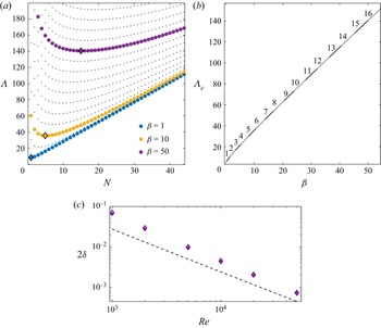
Figure 1 shows the neutral curves for various wavenumbers  $\beta$ where
 $\varLambda$ is shown as a function of
 $N$ in figure 1(a). For a given value of
 $\beta$, the value of
 $N$ that minimises
 $\varLambda$ satisfies
 $\beta ^2=N^3(3 + 2 N)/ (4 + 3 N)$. Since
 $N$ must be an integer, the most dangerous mode will correspond to
 $N=1$ when
 $\beta < 2^{1/2}$ and to an integer value number
 $N\approx [(3/2)\beta ^2]^{1/3}$ for large
 $N$. Figure 1(b) displays
 $\varLambda _c=\min _{N}\varLambda$ as a function of
 $\beta$. Numbers above solid/dashed curves indicate the value of
 $N$ that minimizes
 $\varLambda$ for a given
 $\beta$ which corresponds to the most dangerous mode.
(a) Plot of  $\varLambda$ vs
 $N$ for given
 $\beta$ values. Black markers show the minimum
 $\varLambda$ values to indicate the most dangerous modes
 $N=1$, 5, 15 for
 $\beta =1$, 10, 50, respectively. (b) Plot of
 $\varLambda _c$ vs
 $\beta$ where numbers over solid/dashed curves indicate the most dangerous mode. (c) Critical
 $\delta$ value as a function of
 $Re$ for
 $N=3$ (red) and
 $N=4$ (blue) in comparison to the expected asymptotic scaling given by (2.11) and (2.20) (for
 $N=3$,
 $\beta =10$) shown by dashed line.

Figure 1(c) displays independent calculations of wall transpiration amplitudes that lead to neutral stability of the base flow as a function of  $Re$. These calculations were performed at
 $\beta =10$ for disturbances with
 $N=3$ and
 $N=4$ via full linearized Navier–Stokes calculations; see Blackburn (Reference Blackburn2002) and Barkley, Blackburn & Sherwin (Reference Barkley, Blackburn and Sherwin2008). We see that the asymptotic and numerical solutions are in progressively better agreement as
 $Re$ increases but it is interesting to note that the agreement is not as good as found in the planar case by Hall (Reference Hall2022). We expect that agreement would be improved by continuing the expansion to higher order but our emphasis here is on the nonlinear problem and so we do not do so.
3. The numerical solution of the full interaction equations
Our computational approach is based on the numerical formulation described in Ozcakir et al. (Reference Ozcakir, Tanveer, Hall and Overman2016), which uses a Galerkin truncation of Fourier modes in  $\theta$ and a Chebyshev representation in
 $r$ with appropriately chosen velocity functions
 $\varPhi _j$,
 $\varPsi _j$ satisfying no-slip boundary conditions. Here, we give a brief discussion of the key elements that are added to the existing solver for the present problem. Within the core, the nonlinear equations (2.3) describing the roll–streak flow are solved numerically. It is convenient to decompose the velocity field
 $(u,v,w)$ as
 \begin{equation} (u,v,w)={\boldsymbol v}_B+{\boldsymbol V}(r,\theta), \end{equation}
where  ${\boldsymbol v}_B(r,\theta )$ is a solenoidal base velocity field satisfying the boundary conditions (2.12) which includes Hagen–Poiseuille flow,
 ${\boldsymbol V}(r,\theta )$ is the perturbation velocity with no-slip boundary conditions. Using (3.1) in equations (2.3), one obtains
 \begin{equation} {\boldsymbol V} \boldsymbol{\cdot} \boldsymbol{\nabla} {\boldsymbol V}+ {\boldsymbol v}_B \boldsymbol{\cdot} \boldsymbol{\nabla} {\boldsymbol V}+ {\boldsymbol V}\boldsymbol{\cdot} \boldsymbol{\nabla} \boldsymbol v_B + \boldsymbol{\nabla} p-\nabla^2 {\boldsymbol V} = \nabla^2 {\boldsymbol v}_B - {\boldsymbol v}_B \boldsymbol{\cdot} \boldsymbol{\nabla} {\boldsymbol v}_B, \end{equation}
where  $p(r,\theta )$ is the perturbation pressure. This formulation allows us to find
 $N$-fold rotationally symmetric (
 $\mathbb {R}_{N}$) solutions
 ${\boldsymbol V}(r,\theta )$ using the truncated basis representations
 \begin{equation} \boldsymbol{V}\approx\sum[{u}_{jk} \varPhi_j ({ r};k N) \cos{k N \theta}, {v}_{jk} \varPhi_j ({ r};k N) \sin{k N \theta}, {w}_{jk} \varPsi_j ({r};k N) \cos{k N \theta}] \end{equation}
for the radial, azimuthal and axial perturbation velocity components, where  $\varPhi _j$,
 $\varPsi _j$ are given in terms of Chebyshev polynomials
 $T_{j}$ as
 \begin{equation} \varPhi_j (r; k) =\begin{cases} T_{2j+2} (r) - T_{2j} (r) & \text{if } k \text{ is odd},\\ T_{2j+3} (r) - T_{2j+1} (r) & \text{if } k \text{ is even}, \end{cases} \end{equation}
and
 \begin{equation} \varPsi_j (r; k) =\begin{cases} T_{2j+3} (r) - T_{2j+1} (r) & \text{if } k \text{ is odd},\\ T_{2j+2} (r) - T_{2j} (r) & \text{if } k \text{ is even}. \end{cases} \end{equation}
It should be noted that this representation of  $\varPhi _j$ and
 $\varPsi _j$ forms a complete radial basis for the boundary value problem. The sums are taken over
 $j\in [0, J]$ and
 $k\in [0, M]$ for large enough integer values of
 $J$ and
 $M$ to obtain three-digit relative accuracy for each velocity component in the solution. The cos/sin basis functions are chosen to fix the azimuthal phase of the flow structure. Note that the relative phase in
 $\theta$ between the radial and azimuthal velocity components is fixed by continuity. The relative phase of the streamwise velocity component is then determined through the ‘lift-up’ effect term
 $u \partial w/\partial r$ in (2.3c). Inserting this basis with given
 $N$,
 $\beta$ and
 $\varLambda$ into (3.2) produces a nonlinear algebraic system for
 $\{u_{jk},v_{jk},w_{jk} \}$, which is solved via Newton's method and the generalized minimal residual method.
For given  $N,\beta$, we determine
 $\varLambda _0$ at which the flow becomes unstable using the linear stability results of § 2. A small amplitude neutral eigenfunction is then used as an initial guess in the Newton iteration procedure near this neutrally stable point
 $\varLambda =\varLambda _0$. At each Newton step, the linear ordinary differential equation (2.9) is solved using spectral methods for coefficients
 $\{p_k,1< k< M\}$, where
 $P(\theta )=\sum p_k \sin {k N \theta }$. The resulting
 $P(\theta )$ is then used to generate boundary conditions (2.12) which in turn are used to construct the base flow
 ${\boldsymbol v}_B(r,\theta )$. Once a converged solution is found, an arc-length continuation procedure with continuation parameter
 $\varLambda$ is used to determine other solutions. The corresponding eigenvalue problems were solved numerically using an Arnoldi method.
4. Results
In order to describe the results over a range of wavenumbers of physical interest we consider the wavenumbers  $\beta =1,10, 50$. Results at smaller values of
 $\beta$ than these are perhaps less physically relevant since the implementation of transpiration over long lengths of pipe would be difficult. We restrict attention to solutions that possess shift-reflect symmetry calculated in an
 $\mathbb {R}_{N}$-symmetric subspace.
We first examine the bifurcation structure near the value of  $\varLambda$ where instability first occurs for a given
 $\beta$. Therefore, we consider the modes
 $N=1$, 5, 15 which are the most unstable modes for
 $\beta =1$, 10, 50, respectively; see figure 1(a,b).
In figure 2 we display the evolution of the streak component of the solutions. For a given  $N$-fold solution, the streak associated with the flow is defined as the axial component of the solution excluding the Hagen–Poiseuille solution
 $(1-r^2)\boldsymbol {\hat {z}}$ and it can be written as
 $\sum _{k=0}^{M}{w}_{k}(r) \cos {k N \theta }$. Therefore, the streak amplitude of the
 $kN$th mode is measured by
 $A_k=\max _{r_j} |w_k(r_j)|$, where
 $\{r_j\}$ is the set of radial collocation points. For each solution, we plot
 $A_k$ as a function of
 $\varLambda$ for the first four or five harmonics. Such amplitude plots are useful when we wish to understand how different modes contribute to the total energy of the streak as the transpiration amplitude
 $\varLambda$ is varied. Also, these provide a convenient way to highlight how symmetry-breaking bifurcations occur as the values of
 $A_k$ vanish at the bifurcation points for some values of
 $k$.
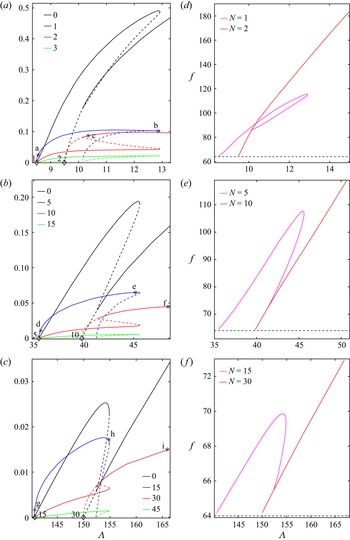
(a–c) Streak modal amplitudes  $A_k$ vs
 $\varLambda$ for solutions to (2.3) arising at their neutral
 $\varLambda$ value (diamond markers) for (a)
 $\beta =1$ and
 $N=1$, 2, (b)
 $\beta =10$ and
 $N=5$, 10, (c)
 $\beta =50$ and
 $N=15$, 30. Here
 $A_k$s values are shown for the first four
 $k$-modes. Solid/dashed lines indicate where the solution is stable/unstable. Figure 3 presents flow profiles corresponding to the solutions where the fundamental modes are labelled here. (d–f) Darcy friction factors corresponding to the two leading modes of (a–c), respectively; the dashed line represents the Hagen–Poiseuille value
 $f=64$.

Figure 2(a) displays the solution branches for the  $N=1$ and
 $N=2$ solutions bifurcating from the neutral
 $\varLambda$ values on the abscissa for the case
 $\beta =1$. The solid/dashed curves indicate the regions where the solution is stable/unstable. The
 $N=1,2$ solutions originate as supercritical bifurcations at the linear instability points at
 $\varLambda \approx 8.485$, 9.487, respectively. Initially, the highest amplitudes are in the fundamental modes
 $A_1$ and
 $A_2$ for the
 $N=1$ and
 $N=2$ solutions, respectively. As
 $\varLambda$ increases, the mean flow as represented by
 $A_0$ grows rapidly and becomes the dominant part of the streak. The
 $N=1$ solution bifurcates supercritically into a stable solution which subsequently loses stability at a saddle-node point and then continues as an unstable solution with
 $\varLambda$ decreasing. That branch then joins the
 $N=2$ solution as a symmetry-breaking secondary bifurcation from that solution. At that point, the
 $A_0$ and
 $A_2$ modes join the
 $A_0$ and
 $A_2$ curves of the
 $N=2$ solution branch, while all the
 $A_k$ modes with odd
 $k$ decrease to zero. After the latter bifurcation, the pure
 $N=2$ mode becomes stable. Thus, the most unstable mode to bifurcate does so supercritically but then loses stability at a saddle-node point with the lower branch then joining the second mode to bifurcate. At that point the second mode to bifurcate is stabilized. If the control parameter is slowly increased in an experiment by say increasing
 $Re$, then the finite amplitude solution which initially bifurcates would be followed to the saddle-node point where it would then jump down to the stable part of the branch corresponding to the second mode. However, starting with a stable mode on the second mode stable branch and decreasing
 $\varLambda$, hysteresis would be observed.
The behaviour described above was found to be typical of the bifurcation structure found for other values of  $\beta$ immediately after the first onset of instability. Thus, the first mode to become unstable bifurcates supercritically but then reaches a saddle-node point before continuing back to lower values of
 $\varLambda$ and terminating as a secondary bifurcation of the second mode to become unstable. Therefore, the behaviour shown in figure 2(b,c) for
 $\beta =10,15$ is similar to that described above for
 $\beta =1$.
Figure 2(d–f) displays the Darcy friction factor
 \begin{equation} f=\frac{64}{(2 \bar{w})^2}, \end{equation}
where  $\bar {w}= {\rm \pi}^{-1}\iint w(r,\theta ) r\, \mathrm {d} r \,\mathrm {d} \theta$ is the bulk velocity associated with the solutions shown in figure 2(a–c), respectively. The corresponding value for Hagen–Poiseuille flow,
 $f=64$, is shown as a dashed line. We observe that if
 $f>64$, transpiration reduces the bulk velocity below the value
 $\bar {w}=0.5$ appropriate to Hagen–Poiseuille flow. These plots exhibit similar bifurcation structures for all values of
 $\beta$, similar to the behaviour observed for the corresponding
 $A_0$ vs
 $\varLambda$ plots. From the onset of first instability, the friction factor of the first mode increases until it reaches a saddle-node value at which point the locus changes direction and subsequently
 $f$ decreases with decreasing
 $\varLambda$ until it reaches the Hagen–Poiseuille value at the secondary bifurcation point. For the second mode solution branch, the friction then continues to increase indefinitely within our calculation range. As these results indicate higher friction factors with transpiration in comparison to Hagen–Poiseuille flow, they suggest significant drag increase due to transpiration. The drag decreases with increasing
 $\beta$ with the largest drag observed for the
 $N=2$ solution branch when
 $\beta =1$. We note that since Hagen–Poiseuille flow satisfies the Stokes equations, it also provides the minimum viscous dissipation for a given streamwise mean pressure gradient and viscosity. Hence, any finite amplitude disturbance to it necessarily results in greater drag.
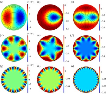
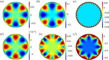
The cross-sectional velocity profiles of the solutions at points labelled as (a–i) on figure 2 are shown in figure 3(a–i). Solutions are constructed using all Fourier modes but the labels (a–i) are marked only on the fundamental modes for visual clarity. In all plots the contours represent the streak part of the flow and black curves indicate sectional streamlines of the roll flow. Figure 3(a) shows the solution labelled (a) on figure 2(a) where the solution is almost linear and the streak field resembles the eigenmode obtained by the linear stability analysis. As nonlinearity grows, solutions take the form shown in figure 3(b) at the largest value of  $\varLambda$ for the
 $N=1$ solution which is labelled (b) on figure 2(a). Following the continuation locus as
 $\varLambda$ decreases, the
 $N=1$ solution disappears and joins the
 $N=2$ solution branch. Figure 3(c) displays the flow beyond this bifurcation point on the
 $N=2$ solution branch (labelled c on figure 2a). The same flow behaviour is shown in figure 3(d–f) for
 $\beta =10$, and in figure 3(g–i) for
 $\beta =50$. For all the calculations, far from the bifurcation point, the flow is characterised by
 $N$ localised fast streaks (red) near the wall with each of them trapped between two slow streaks (blue). As
 $\beta$ becomes larger, these fast/slow streaks move away from the centre of the pipe towards the wall as solutions become more nonlinear with higher modes becoming more active.
The cross-sectional velocity field  ${\boldsymbol v}_B(r,\theta )+{\boldsymbol V}(r,\theta )$ at points labelled in figure 2. Contours indicate axial/streak velocity component intensity as indicated by the colourbars and lines show sectional streamlines of the roll flow when
 $\beta =1$ on (a–c),
 $\beta =10$ on (d–f) and
 $\beta =50$ on (g–i).

For a given value of  $\beta$ as
 $\varLambda$ increases, successively more modes become unstable and the bifurcation structure involving all possible modes is prohibitively expensive to compute. Thus, for example, when
 $\beta =50$, the modes
 $N=4,5,\ldots,44$ are all linearly unstable when
 $\varLambda =169$. For a given value of
 $N$, it would be necessary to carry the first
 $64$ harmonics to resolve the solution and so a resolution of the bifurcation structure in the latter scenario would require at least
 $64\times 44$ azimuthal modes.
Now we present results of relevance to travelling wave solutions which are known to exist in the absence of transpiration; see Ozcakir et al. (Reference Ozcakir, Tanveer, Hall and Overman2016). In particular, we focus on  $N=4$ solutions known to exist without transpiration; those earlier computations showed that, for
 $N=4$, complex interactions occur for large
 $\beta$ values. We here examine some specimen calculations with transpiration when
 $\beta =10$ and
 $\beta =50$ for which the bifurcation diagrams are shown in figure 4.
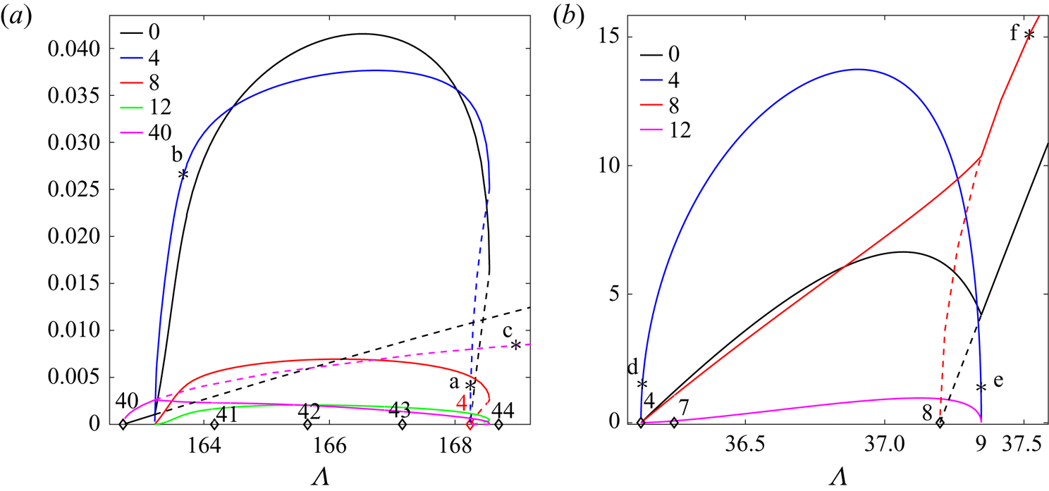
Streak amplitude  $A_k$ vs
 $\varLambda$ for (a)
 $\beta =50$ and
 $N=4$, 40 and (b) for
 $\beta =10$ and
 $N=4$, 8. Diamond markers on the abscissae indicate neutral
 $\varLambda$ values at which new solutions arise. Solid/dashed lines indicate where the solution is stable/unstable. Figure 3 shows flow profiles corresponding to the solutions where the fundamental modes are labelled here.

The markers on the abscissae of figures 4(a) and 4(b) indicate neutral values of  $\varLambda$ at which new
 $N$-fold solutions arise. The numbers above each marker give the value of
 $N$. In figure 4(a) black markers indicate bifurcation points for the solutions
 $N=40\text {--}44$ while the red marker shows the neutral value for
 $N=4$ trapped between
 $N=43$ and
 $N=44$ for
 $\beta =50$. Following the continuation locus for
 $N=40$, it may be seen that soon after the unstable
 $N=40$ solution arises at the neutral value,
 $\varLambda \approx 162.7$, the
 $N=4$ solution branches from it as a secondary bifurcation at
 $\varLambda \approx 163.3$. After this value, both solutions are stable in the
 $\mathbb {R}_{4}$ subspace and exist together until
 $\varLambda <168.5$. The
 $N=4$ solution does not continue to exist beyond
 $\varLambda =168.5$. In order to illustrate how the
 $N=4$ solution evolves, the cross-sectional velocity profiles for the points labelled (a–c) in figure 4(a) are shown in figure 5(a–c). Near onset, the
 $N=4$ solution resembles the linear eigenmode (figure 5a); during continuation, higher modes develop near the wall (figure 5b) and the
 $N=40$ solution is approached (figure 5c).
The cross-sectional velocity field  ${\boldsymbol v}_B(r,\theta )+{\boldsymbol V}(r,\theta )$ at points labelled in figure 4. Contours indicate axial/streak velocity component intensity as indicated by the colourbars and lines show sectional streamlines of the roll flow for
 $\beta =50$ on (a–c), and for
 $\beta =10$ on (d–f).

Figures 4(b) and 5(d–f) describe the analogous behaviour for  $\beta=10$ where
 $N=4$ and
 $N=8$ solutions arise as instabilities of the modified base flow at about
 $\varLambda \approx 36.12$ and
 $\varLambda \approx 37.2$, respectively. As indicated by solid/dashed lines, the
 $N=4$ solution is always stable whereas the
 $N=8$ solution has one unstable mode in the
 $\displaystyle \mathbb {R}_{4}$ subspace initially. At
 $\varLambda \approx 37.34$, the growth rate of the unstable mode changes sign at which point
 $N=4$-symmetric solutions are born out of symmetry-breaking bifurcations from the eight-fold solutions. Beyond this point, the
 $N=8$ solutions are stable. The results shown in figure 4(a) show then that when linearly unstable modes with low and high values of
 $N$ coexist then, unlike the tendency observed in figure 2, the mode with the higher
 $N$ can suffer a secondary bifurcation to a stable lower
 $N$ mode. By comparison, figure 4(b) shows that, as in figure 2, the tendency is for the first mode to bifurcate supercritically but remaining stable only for a finite range of
 $\varLambda$. However, the first harmonic of the latter mode bifurcates supercritically into an unstable mode at a higher
 $\varLambda$ before becoming stable after a secondary bifurcation.
5. Discussion and conclusions
In this work Hagen–Poiseuille flow modified by transpiration applied at the wall is considered and solutions of the full nonlinear interaction equations have been computed numerically for a number of cases. The interaction equations are derived on the assumption that the Reynolds number is large and the transpiration velocity at the wall is small compared with the centreline flow. The solution of the linearized interaction equations gives predictions of the neutral configuration in strong agreement with solutions of the linearized Navier–Stokes equations and this suggests the asymptotically reduced problem applies to situations of practical importance. The neutral configuration and the corresponding eigenfunctions depend strongly on the streamwise wavenumber  $\beta$ of the transpiration. Thus, as the transpiration wavelength decreases, the most dangerous azimuthal mode number
 $N$ increases so that the disturbance varies on an increasingly short length scale.
The strongly nonlinear states we have calculated differ in significant ways from the exact coherent states which occur in the absence of transpiration. Firstly, the states discussed here are driven by a stationary wave system. The Reynolds stresses driving the roll–streak flow are therefore concentrated near the wall rather than in the viscous critical layer of the moving waves of exact coherent structures in the absence of transpiration. Thus, the roll–streak field here is driven by an azimuthal velocity jump across the viscous wall layer rather than a viscous critical layer. We note however that if the transpiration wave is travelling with a speed of size  $Re^{-1/3}$ then the interaction problem is identical to that considered here.
In the nonlinear regime it is found that the first mode to bifurcate does so supercritically but then becomes unstable to a higher mode. A complete picture of the bifurcation structure for even moderately large values of  $\beta$ is difficult because of the high number of azimuthal modes needed to resolve the disturbance. However, we can make some quite general conclusions based on the limited calculations carried out. Firstly consider the results of figures 2 and 4(b). These cases correspond to situations when the most unstable mode at the given
 $\beta$ does not correspond to an almost equally unstable mode at a much smaller
 $N$ value. In that case the tendency is for the available stable states to be associated with progressively higher
 $N$ values as
 $\varLambda$ increases. In contrast, for a situation like that in figure 4(a) with the most unstable mode
 $N=40$ only slightly more unstable than the mode
 $N=4$, then it is possible for the lower modes to become stable as
 $\varLambda$ increases.
The fundamental building block of exact coherent structures, the roll–streak field, is identical with or without transpiration and is driven by a vortex-wave interaction in both cases. The close relationship of the sustaining mechanisms for exact coherent structures with and without transpiration suggests that transpiration might well have a significant effect on fully turbulent flows. This points to the possible importance of transpiration to control turbulence by preferentially exciting less dissipative underlying flow patterns. Certainly it is now well established that suction is a viable means to control boundary layer transition but the engineering difficulties associated with producing a wavelike transpiration distribution velocity field are challenging.
Figures 3 and 5 show that the mean departure from Hagen–Poiseuille flow, i.e. the axial flow perturbation averaged over  $(r, \theta )$, is in most cases negative, so that the drag on the pipe will be increased by transpiration, as is also evident in figure 2(d–f). That is also the case with known exact coherent structures in the absence of transpiration so it is of interest to determine if that drag can be modified by transpiration. In order to address that issue the interaction equations must be augmented by the jump condition associated with VWIa, solutions of the augmented system will show whether transpiration can be used to preferentially excite transpiration-free known exact coherent structure states.
Finally we comment on what implications the present work may hold for the related problem where the basic instability is caused by radial wall undulations rather than transpiration. For channel flows, Hall (Reference Hall2022) showed that the linear stability problems are quite similar, but beyond noting wall undulations of size  $O(Re^{1/3})$ larger than the transpiration amplitude are needed to promote instability, a direct link between the problems is not possible. That follows from the fact that, for the undulation problem, the forcing term in the pressure equation differs from that for the transpiration case. Thus, in the equivalent of (2.9) for the undulating wall case the forcing term on the right-hand side is proportional to
 $\lambda ^{5/3}$ rather than
 $\lambda$.
Funding
This research was supported by Australian Research Council Discovery Project grant DP170104703.
Declaration of interests
The authors report no conflict of interest.