


1 Introduction
Reaction–diffusion equations have been used to describe mechanisms for spatiotemporal dynamics in ecological systems where dispersal of individuals in the considered population follows random diffusion [Reference Cantrell and Cosner9, Reference Murray21–Reference Okubo and Levin23, Reference Shigesada and Kawasaki28, Reference Skellam29]. Significant progress has been made for the propagation dynamics of biological invasion since the pioneering work of Aronson and Weinberger [Reference Aronson and Weinberger2, Reference Aronson and Weinberger3] on the Fisher-KPP equation
 $ u_t = u_{xx} + f(u), \forall (t,x)\in (0,+\infty )\times \mathbb {R}, $
where
 $u(t, x)$
represents the density of the species at time t and location x; function f is
 $C^1-$
smooth,
 $f(0)=f(1)=0$
,
 $f(u)>0$
for
 ${u\in (0,1)}$
and
 $f(u)\leq f'(0)u$
for
 $u\geq 0$
. It is known that the asymptotic spreading speed
 $c_{KPP} = 2\sqrt {f'(0)}$
coincides with the minimal speed of traveling waves. Reproductive synchrony of some plant and animal populations (e.g., fish, dandelions, or large mammals), where individuals give birth only at the beginning of each period, motivates the study of the impulsive reaction–diffusion system:
 $$ \begin{align*} \begin{cases} u_t^{(m)}=u^{(m)}_{xx}+f(u^{(m)}),&t\in(0,T],x\in\Omega,\\ u^{(m)}(0,x)=g(N_m(x)),&x\in\Omega,\\ N_{m+1}(x)=u^{(m)}(T,x),&x\in\Omega, \end{cases} \end{align*} $$
where
 $g(u)$
is the (continuous) birth function. Lewis and Li [Reference Lewis and Li15] showed that such a system has a threshold, related to the domain size, that can be used to characterize the extinction or persistence of the species for bounded domain
 $\Omega $
with
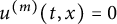 $u^{(m)}(t,x) = 0$
for
 $x \in \partial \Omega $
. They also showed that the minimal speed
 $ c_{Imp} = 2\sqrt {f'(0) + \frac {1}{T} \ln g'(0)} $
(see Lin and Wang [Reference Lin and Wang18] for a general response term
 $f(u)$
). See [Reference Vasilyeva, Lutscher and Lewis32] for a non-local impulsive version of the model formulated to study the population dynamics in a stream and to examine how advection affects population persistence. See also [Reference Fazly, Lewis and Wang13, Reference Fazly, Lewis and Wang14] for impulsive models in higher dimensions, and recent studies in [Reference Bai, Lou and Zhao4, Reference Buedo-Fernández and Faria8, Reference Faria and Figueroa12, Reference Meng, Lin and Pedersen20, Reference Wang, Zhang and Huang34–Reference Wang, Salmaniw and Wang36, Reference Wang and Wang38, Reference Wu and Zhao40].
Another relevant line of research has been driven by the impact of climate change on species persistence [Reference Alan Pounds, Bustamante, Coloma, Consuegra, Fogden, Foster, La Marca, Masters, Merino-Viteri, Puschendorf, Ron, Sánchez-Azofeifa, Still and Young1, Reference Stanton, Shoemaker, Pearson and Akçakaya30, Reference Thomas, Hill, Anderson, Bailey, Beale, Bradbury, Bulman, Crick, Eigenbrod, Griffiths, Kunin, Oliver, Walmsley, Watts, Worsfold and Yardley31]. Potapov and Lewis [Reference Potapov and Lewis25] developed a population dynamic model in a climate-driven shifting environment
 $u_t= u_{xx}+f(x-ct,u), \forall (t,x)\in (0,+\infty )\times \mathbb {R},$
where
 $c>0$
is the speed caused by climate changes. For the scenario where a supportive environment is encircled by adverse ones, they derived the minimum habitat size required for the persistence of the species. Subsequent studies [Reference Berestycki, Diekmann, Nagelkerke and Zegeling5, Reference Berestycki and Rossi7, Reference Li, Bewick, Shang and Fagan16, Reference Shen, Shen, Xue and Zhou26, Reference Shen and Xue27, Reference Vo33] motivated this pioneering work. In addition, Berestycki and Fang [Reference Berestycki and Fang6] considered the situation where a favorable environment on the left half of a plane expands into an unfavorable environment on the right at the shifting speed
 $c> 0$
. Other developments include studies [Reference Berestycki, Diekmann, Nagelkerke and Zegeling5, Reference Berestycki and Rossi7] linking the global dynamics, the forced waves (e.g., [Reference Berestycki and Rossi7, Theorem 3.6]) and the study by Fang et al. [Reference Fang, Peng and Zhao10] on the propagation dynamics in time-periodic environment; as well as the paper [Reference Zhang and Zhao41] for propagation dynamics involving nonlocal dispersal.
Consideration of the effects of habitat shifting on the propagation of species with birth pulse in high-dimensional spaces leads to the following model:
 $$ \begin{align} \begin{cases} u_t^{(m)}=u^{(m)}_{xx}+f(x-cte,u^{(m)}),&t\in(0,1],x\in\mathbb{R}^n,\\ u^{(m)}(0,x)=g(N_m(x)),&x\in\mathbb{R}^n,\\ N_{m+1}(x)=u^{(m)}(1,x),&x\in\mathbb{R}^n. \end{cases} \end{align} $$
The studies [Reference Wang and Wang37, Reference Zhang, Yi and Chen42, Reference Zhang, Yi and Wu43] established the threshold dynamics in bounded domains, analyzed the properties of positive steady states, and demonstrated how the shifting speed c along with the impulsive reproduction rate g influences the persistence of the population. These studies ignore the dependence of the growth rate
 $r(t,x)$
in seasonal succession. Incorporating this T-periodic growth rate
 $r(t,x)$
and the occurrence of birth pulses at points
 $kT$
(
 $k = 0, 1, 2, \dots $
), naturally, it leads to the following Fisher-KPP equation with a time-periodic environment and birth pulse:
 $$ \begin{align} \begin{cases} u_t=u_{xx}+u(r(t,x-ct)-u),&t\in(kT^+,(k+1)T],x\in\mathbb{R},\\ u(kT^+,x)=g(u(kT,x)),&x\in\mathbb{R},k\in\mathbb{N},\\ u(0,x)=u_0(x),&x\in\mathbb{R}, \end{cases} \end{align} $$
where
 $r(t, x - ct)$
, with
 $r(t+T, x) = r(t, x)$
, denotes the growth rate of species in a time-periodic shifting environment with speed c; the function
 $g(\cdot )$
describes a birth pulse occurring at the start of each period; the initial function
 $u_0(x)$
is nonnegative, bounded, and continuous. For
 $t \in (kT^+, (k+1)T]$
in the first equation of (1.2), u satisfies the equation for
 $t \in (kT, (k+1)T]$
with the initial value
 $u(kT^+, x)$
, which is the right-hand limit of u at
 $t = kT$
. Hence, we provide a systematic description of the dynamics of model (1.2).
Throughout the remainder of this article, we assume that
 $r(t,x)$
is continuous, bounded on
 $\mathbb {R}^2$
, non-increasing in x, and has the following property to reflect that the environment is supportive at local
 $-\infty $
and adverse at local
 $+\infty $
:
-
(R): the limits
 $r(t,+\infty )$
and
$r(t,-\infty )$
exist uniformly in t, and
$r(t,+\infty )<0<r(t,-\infty )$
.



In addition, we assume:
-
(G1):
$g(u)$
is continuous and non-decreasing, locally Lipschitz continuous uniformly in
$u\geq 0$
; -
(G1):
$g(0)=0$
;
$g'(0)$
exists;
$g(u)/u$
is non-increasing and
$g(u)>0$
in
$u>0$
; -
(G1): there is
$N>0$
such that
$\frac {g(N)}{N}\leq 1$
; -
(G1): there exist
$D,\rho> 1$
and small
$\delta>0$
satisfying
$g(u)\geq g'(0)u-Du^\rho $
for
$u\in [0,\delta ]$
.




We will show the existence and exponential stability of forced KPP waves, and investigate the global dynamical behaviors of (1.2). Herein, the term “forced” signifies that the propagation speed c of the KPP wave is externally prescribed by the drift speed of the heterogeneous environment, rather than being an intrinsic wave speed selected by the system. We first define a forced KPP wave by considering
 $u(t,x)=U(t,x-ct)$
. Let
 $\xi =x-ct$
. Note that
 $U(t,\xi )$
satisfies
 $$ \begin{align} &U_t=U_{\xi\xi}+cU_\xi+U(r(t,\xi)-U), t\in(kT^+,(k+1)T],\xi\in\mathbb{R}; \end{align} $$
 $$ \begin{align} &U(kT^+,\xi)=g(U(kT,\xi)), k\in\mathbb{N},\xi\in\mathbb{R}; \end{align} $$
 $$ \begin{align} &U(t+T,\xi)=U(t,\xi), t\in(kT^+,(k+1)T],\xi\in\mathbb{R}. \end{align} $$
Then,
 $U(t,\xi )$
is a forced KPP wave of (1.2) when
 $$ \begin{align} U(t,+\infty)=0 \text{ and } U(t,-\infty)=p(t). \end{align} $$
Here,
 $p(t)$
satisfies (2.2) when
 $e^{\bar {r}(-\infty )}[g'(0)]^{\frac {1}{T}}>1.$
Note that (1.2) is discontinuous at
 $t=kT$
due to the birth pulse. Unlike the continuous time-periodic system considered in [Reference Fang, Peng and Zhao10], the corresponding Poincaré map of (1.2) has different properties. Constraints must be imposed on the birth pulse g to ensure that the Poincaré map remains bounded. Moreover, we establish a comparison principle and construct appropriate upper and lower solutions. In studying the propagation dynamics, we apply the principal eigen-pair of the eigenvalue problem for the corresponding linearized equation, along with iteration methods, to prove the results when
 $c \leq -c^*$
. This approach differs from that in [Reference Fang, Peng and Zhao10] as we will have to consider the birth pulse.
The article continues with the following structure. In Section 2, we provide some preliminaries about the limit systems and some a-priori estimates for possible forced waves. In Section 3, we consider the forced KPP waves and analyze the spreading properties of solutions to (1.2) with different speeds c. In Section 4, we present some numerical simulations, and in the final section, we present some discussions.
2 Preliminaries
2.1 Two periodic problems
In this section, we summarize some preliminary results which will be used in subsequent analysis. We first consider the limiting equation
 $$ \begin{align} \begin{cases} u_t=u(r(t,-\infty)-u),&t\in(kT^+,(k+1)T],\\ u(kT^+)=g(u(kT)),&k\in\mathbb{N},\\ u(0)=u_0>0. \end{cases} \end{align} $$
By the classical theory of ODEs, (2.1) admits a unique classical solution. We establish a threshold result for system (2.1).
Lemma 2.1 Let
 $\alpha (t;u_0)$
be the unique solution of (2.1) with initial value
 $u_0>0$
and define
 $\bar {r}(-\infty )=\frac {1}{T}\int _0^T r(t,-\infty )dt$
.
-
(1) If
$e^{\bar {r}(-\infty )}[g'(0)]^{\frac {1}{T}}\leq 1$
, then (2.1) has only the zero solution. -
(2) If
$e^{\bar {r}(-\infty )}[g'(0)]^{\frac {1}{T}}>1$
, then
$\alpha (t;u_0)>0$
satisfies
$\lim \limits _{t\to +\infty }|\alpha (t;u_0)-p(t)|=0.$
Here,
$p(t)>0$
is the unique solution of (2.2)
$$ \begin{align} \begin{cases} u_t=u(r(t,-\infty)-u),&t\in(0^+,T],\\ u(0^+)=g(u(0)),\\ u(0)=u(T). \end{cases} \end{align} $$






Proof By [Reference Zhao44, Theorem 2.3.4], we only show
 $\lim \limits _{t\to +\infty }|\alpha (t;u_0)-p(t)|=0$
. The proof of [Reference Meng, Ge and Lin19, Theorem 3.4] implies that (2.2) has a unique solution
 $p(t)$
. For given
 $u_0>0$
, there are
 $\epsilon>0$
and
 $C>\max \{N,\max _{[0,T]}r(t,-\infty )\}$
such that
 $\epsilon <u_0<C$
. Choose a large enough
 $K>0$
such that
 $u(r(t,-\infty )-u)+Ku$
is increasing in u. Define
 $\{w^{(m)}\}_{m\geq 0}$
satisfying
 $$ \begin{align*} \begin{cases} w^{(m)}_t+Kw^{(m)}=Kw^{(m-1)}+w^{(m-1)}(r(t,-\infty)-w^{(m-1)}),&t\in(0^+,T],\\ w^{(m)}(0^+)=g(w^{(m-1)}(0)),\\ w^{(m)}(0)=w^{(m-1)}(T), \end{cases} \end{align*} $$
with
 $w^{(0)}\equiv C$
. Obviously,
 $0<w^{(m+1)}\leq w^{(m)}\leq \cdots \leq w^{(1)}\leq w^{(0)}\equiv C.$
Then, there is
 $w^*(t)$
satisfying (2.2) such that
 $\lim \limits _{m\to +\infty }w^{(m)}(t)=w^*(t),\forall t\in [0,T]. $
By the uniqueness,
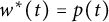 $w^*(t)=p(t)$
. Observed that
 $\alpha (t;u_0)\leq \max \{N,\max _{[0,T]}r(t,-\infty )\}< C=w^{(0)}$
, then
 $\alpha (T;u_0)\leq w^{(0)}(T)=w^{(1)}(0)$
, so
 $ \alpha (T^+;u_0)=g(\alpha (T;u_0))\leq g(w^{(0)}(T))=w^{(1)}(0^+). $
By comparison principle, we follows from the iteration methods that
 $\alpha (t+mT;u_0)\leq w^{(m)}(t), \forall t\in [0,T],$
for
 $m = 0, 1, 2, \ldots $
. Then,
 $\lim \limits _{m\to +\infty }\alpha (t+mT;u_0)\leq \lim \limits _{m\to +\infty }w^{(m)}(t)=p(t).$
Similarly, we can find an increasing sequence
 $\{v^{(m)}\}_{m\geq 0}$
satisfying
 $$ \begin{align*} \begin{cases} v^{(m)}_t+Kv^{(m)}=Kv^{(m-1)}+v^{(m-1)}(r(t,-\infty)-v^{(m-1)}),&t\in(0^+,T],\\ v^{(m)}(0^+)=g(v^{(m-1)}(0)),\\ v^{(m)}(0)=v^{(m-1)}(T), \end{cases} \end{align*} $$
with
 $v^{(0)}\equiv \epsilon $
, such that
 $\lim \limits _{m\to +\infty }\alpha (t+mT;u_0)\geq \lim \limits _{m\to +\infty }v^{(m)}(t)=p(t).$
This completes the proof.
We now consider the eigenvalue problem in bounded domain
 $[l_1,l_2]$
:
 $$ \begin{align} \begin{cases} \phi_t=\phi_{xx}+r(t,-\infty)\phi+\lambda\phi,&t\in(0^+,T],x\in(l_1,l_2),\\ \phi(0^+,x)=g'(0)\phi(0,x),&x\in(l_1,l_2),\\ \phi(t,l_1)=\phi(t,l_2)=0,&t\in[0,T],\\ \phi(0,x)=\phi(T,x)&x\in(l_1,l_2). \end{cases} \end{align} $$
By [Reference Meng, Ge and Lin19, Lemma 2.3], the generalized principal eigenvalue of (2.3) can be written as
 $$ \begin{align} \lambda([l_1,l_2]):=(\frac{\pi}{l_2-l_1})^2-\bar{r}(-\infty)-\frac{1}{T}\ln g'(0). \end{align} $$
We apply the eigenvalue problem (2.3) to discuss the following problem in bounded domain:
 $$ \begin{align} \begin{cases} u_t=u_{xx}+u(r(t,-\infty)-u),&t\in(kT^+,(k+1)T],x\in(l_1,l_2),\\ u(kT^+,x)=g(u(kT,x)),&k\in\mathbb{N},x\in(l_1,l_2),\\ u(t,l_1)=u(t,l_2)=0,&t>0,\\ u(0,x)=u_0(x),&x\in(l_1,l_2). \end{cases} \end{align} $$
Similar to the proof of [Reference Meng, Ge and Lin19, Lemma 2.5], we obtain the following threshold dynamics.
Lemma 2.2 Denote by
 $u(t,x;u_0(x))$
the unique solution of (2.5) with
 $u_0(x)\geq $
and
 $\not \equiv 0$
.
-
(1)
$\lim \limits _{t\to +\infty }u(t,x;u_0(x))=0 \ \text {uniformly in} \ [l_1,l_2]$
if
$\lambda ([l_1,l_2])\geq 0$
. -
(2) For any
$(t,x)\in (0^+,T]\times [l_1,l_2]$
,
$\lim \limits _{m\to +\infty }u(t+mT,x;u_0(x))=u^*(t,x)$
if
$\lambda ([l_1,l_2])< 0$
. Here,
$u^*(t,x)$
satisfies
$$ \begin{align*} \begin{cases} u_t=u_{xx}+u(r(t,-\infty)-u),&t\in(0^+,T],x\in(l_1,l_2),\\ u(0^+,x)=g(u(0,x)),&x\in(l_1,l_2),\\ u(t,l_1)=u(t,l_2)=0,&t\in(0^+,T],\\ u(0,x)=u(T,x),&x\in(l_1,l_2). \end{cases} \end{align*} $$







2.2 Spreading properties of some time-periodic-parabolic problems
At the beginning, we give some definitions for the following equation:
 $$ \begin{align} \begin{cases} u_t=u_{xx}+u(r(t,-\infty)-u),&t\in(kT^+,(k+1)T],x\in\mathbb{R},\\ u(kT^+,x)=g(u(kT,x)),&x\in\mathbb{R},k\in\mathbb{N},\\ u(0,x)=u_0(x)\geq0,&x\in\mathbb{R}. \end{cases} \end{align} $$
Definition 2.3 A T-periodic traveling wave solution of (2.6) is a special solution of the form
 $u(t,x)=W(t, x-ct)$
, where
 $c\in \mathbb {R}$
is the wave speed if
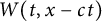 $W(t, x-ct)$
satisfies
 $$ \begin{align*} &W_t=W_{\xi\xi}+cW_\xi+W(r(t,-\infty)-W), t\in(kT^+,(k+1)T],\xi\in\mathbb{R}\\ &W(kT^+,\xi)=g(W(kT,\xi)), k\in\mathbb{N},\xi\in\mathbb{R};\\ &W(t+T,\xi)=W(t,\xi), t\in(kT^+,(k+1)T],\xi\in\mathbb{R} \end{align*} $$
with boundary conditions
 $U(t,+\infty )=0 \text { and } U(t,-\infty )=p(t). $
Moreover, we denote by the downstream spreading speed
 $c^*$
, which coincides with the minimal wave speed for which traveling wave solutions exist.
Remark 2.1 It is crucial to distinguish the concept of a forced KPP wave from that of a traveling wave. A traveling wave is any solution of the form
 $ u(t, x) = W(x - c t) $
, where the speed
 $ c $
is a parameter. In contrast, a forced KPP wave is a very specific type of traveling wave, where the wave speed
 $ c $
is not a free parameter but is externally prescribed by the drift speed. Namely, a forced wave is a traveling wave that is locked to this environmental speed, rather than being a member of a continuum of waves.
According to [Reference Liang, Yi and Zhao17, Theorems 2.2 and 2.3], we can obtain the existence of T-periodic traveling wave and the downstream spreading speed.
Lemma 2.4 If
 $e^{\bar {r}(-\infty )}[g'(0)]^{\frac {1}{T}}>1$
, then there exists a downstream spreading speed
 $$ \begin{align*}c^*:=2\sqrt{\bar{r}(-\infty)+\frac{1}{T}\ln g'(0)}\end{align*} $$
such that, system (2.6) has a T-periodic traveling wave solution
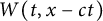 $W(t,x-ct)$
with
 $W(t,-\infty )=p(t)$
and
 $W(t,+\infty )=0$
if and only if
 $c\geq c^*$
.
Remark 2.2 If
 $e^{\bar {r}(+\infty )}[g'(0)]^{\frac {1}{T}}\leq 1$
, then the comparison argument and Lemma 2.1 deduce that, as
 $t\to \infty $
, every nonnegative solution of (2.6) with
 $r(t,-\infty )$
replaced by
 $r(t,+\infty )$
converges to
 $0$
uniformly for
 $x\in \mathbb {R}$
.
In our study here, we consider the following case:
-
(H):
$g'(0)<1<e^{\bar {r}(-\infty )}[g'(0)]^{\frac {1}{T}}$
.

It is easy to see that
 $e^{\bar {r}(+\infty )}[g'(0)]^{\frac {1}{T}}<1<e^{\bar {r}(-\infty )}[g'(0)]^{\frac {1}{T}}$
. Using standard
 $L^p$
theory, together with the upper and lower solution methods, monotone iteration, and the comparison principle, it can be shown that (1.2) has a unique classical solution
 $u(t,x;u_0)$
.
For any given
 $y\in \mathbb {R}\cup \{\pm \infty \}$
, consider
 $$ \begin{align} \begin{cases} U_t=U_{\xi\xi}+cU_\xi+U(r(t,\xi+y)-U),&t\in(kT^+,(k+1)T],\xi\in\mathbb{R},\\ U(kT^+,\xi)=g(U(kT,\xi)),&k\in\mathbb{N},\xi\in\mathbb{R},\\ U(0,\xi)=\phi(\xi),& \xi\in\mathbb{R}, \end{cases} \end{align} $$
where
 $\phi (\xi )\in C(\mathbb {R},\mathbb {R})$
is nonnegative and not identically zero. We first define the generalized upper and lower solutions of (2.7).
Definition 2.5 If there are
 $\{x_i\}_{i=1}^{m}\subset \mathbb {R}$
and function
 $\bar {U}\in C^{1,2}([0,\infty )\times \mathbb {R}\setminus \{x_i\}_{i=1}^{m})$
satisfying
 $$ \begin{align*} \begin{cases} \bar{U}_t\geq \bar{U}_{\xi\xi}+c\bar{U}_\xi+\bar{U}(r(t,\xi+y)-\bar{U}),&t\in(kT^+,(k+1)T],\xi\in\mathbb{R},\\ \bar{U}_x(t,\xi^+)\leq \bar{U}_x(t,\xi^-),& t>0,\xi=x_i,1\leq i\leq m,\\ \bar{U}(kT^+,\xi)\geq g(\bar{U}(kT,\xi)),& k\in\mathbb{N},\xi\in\mathbb{R}, \end{cases} \end{align*} $$
then
 $\bar {U}(t,\xi )$
is called a generalized upper solution of (2.7). A generalized lower solution of (2.7) can be defined by reversing the above inequalities.
When
 $y=0$
, the first equation of (2.7) reduces to (1.3). As
 $y \to \pm \infty $
, the first equation of (2.7) approaches the corresponding limiting equation:
 $$\begin{align*}U_t=U_{\xi\xi}+cU_\xi+U(r(t,\pm\infty)-U), t\in(kT^+,(k+1)T],\xi\in\mathbb{R}. \end{align*}$$
Denote by
 $U^y(t,\xi ;\phi (\cdot ))$
the unique solution of (2.7). Since
 $U^0(t,\xi +y;\phi (\cdot ))$
and
 $U^y(t,\xi ;\phi (\cdot +y))$
are solutions of
 $$ \begin{align*} \begin{cases} U_t=U_{\xi\xi}+cU_\xi+U(r(t,\xi+y)-U),&t\in(kT^+,(k+1)T],\xi\in\mathbb{R},\\ U(kT^+,\xi)=g(U(kT,\xi)),& k\in\mathbb{N},\xi\in\mathbb{R},\\ U(0,\xi)=\phi(\xi+y),& \xi\in\mathbb{R}, \end{cases} \end{align*} $$
the uniqueness implies that
 $$ \begin{align} U^0(t,\xi+y;\phi(\cdot))=U^y(t,\xi;\phi(\cdot+y)),\forall t\geq0, \xi,y\in\mathbb{R}. \end{align} $$
Denote by
 $P_y: C(\mathbb {R},\mathbb {R}^+)\to C(\mathbb {R},\mathbb {R}^+)$
the time-T solution map of
 $U_t=U_{\xi \xi }+cU_\xi +U(r(t,\xi +y)-U), t>0,\xi \in \mathbb {R}.$
Then,
 $Q_y=P_y\circ g$
is the Poincaré map of (2.7) and
 $U^y(kT,\xi ;\phi (\cdot ))=Q_y^{k}(\phi )$
, where
 $Q_y^{k}$
is the kth iteration of
 $Q_y$
. Note that
 $P_y$
meets the properties of [Reference Zhang and Zhao41, Lemma 3.3] or [Reference Fang, Peng and Zhao10, Lemma 2.1]. We first define the local uniform convergence: a sequence of functions
 $\{\phi _n\} \subset C(\mathbb {R}, \mathbb {R}^+)$
converges to
 $\phi $
if for any compact set
 $K \subset \mathbb {R}$
,
 $\sup _{x \in K} |\phi _n(x) - \phi (x)| \to 0$
.
Lemma 2.6
 $Q_y$
satisfies the following conclusions:
-
(1) (Compactness Property) If
$a_n(\xi )$
is uniformly bounded, then
$Q_y[a_n]$
, up to a subsequence, converges locally uniformly. -
(2) If
$\bar {U}(t,\xi )$
and
$\underline {U}(t,\xi )$
are a pair of upper–lower solutions of (2.7) for
$t>0$
and satisfy
$\bar {U}(t,\xi )\geq \underline {U}(t,\xi )$
, then
$$\begin{align*}\underline{U}(0^+,\xi)\leq Q_y(\underline{U}(0,\xi))\leq Q_y(\bar{U}(0,\xi))\leq \bar{U}(0^+,\xi).\end{align*}$$
-
(3)
$Q_y[\phi (\cdot )](\xi +y)=Q_y[\phi (\cdot +y)](\xi ),\forall \xi ,y\in \mathbb {R}$
.





Proof (1) It follows from the third property of [Reference Fang, Peng and Zhao10, Lemma 2.1] that if
 $a_n(\xi )$
is uniformly bounded, then
 $P_y[a_n]$
, up to a subsequence, converges locally uniformly. The hypothesis (G1) ensures that
 $Q_y[a_n]$
also converges locally uniformly. (2) By (G1),
 $g(a_1(\xi )) \leq g(a_2(\xi ))$
for given
 $a_1(\xi ) \leq a_2(\xi )$
. It then follows from the first property of [Reference Fang, Peng and Zhao10, Lemma 2.1] that
 $P_y \circ g(a_1(\xi )) \leq P_y \circ g(a_2(\xi ))$
, namely,
 $Q_y(a_1(\xi )) \leq Q_y(a_2(\xi ))$
. Moreover, we choose a pair of upper and lower solutions of (2.7),
 $\bar {U}(t,\xi )$
and
 $\underline {U}(t,\xi )$
, satisfying
 $\underline {U}(t,\xi ) \leq \bar {U}(t,\xi )$
for
 $t \in (kT, (k+1)T]$
. Since
 $\underline {U}(kT^+, \xi ) \leq g(\underline {U}(kT, \xi ))$
, it follows that
 $$\begin{align*}P_y(\underline{U}(kT^+, \xi)) \leq P_y \circ g(\underline{U}(kT, \xi)) = Q_y(\underline{U}(kT, \xi)).\end{align*}$$
Similarly,
 $Q_y(\bar {U}(kT, \xi )) = P_y \circ g(\bar {U}(kT, \xi )) \leq P_y(\bar {U}(kT^+, \xi ))$
. By the fourth property of [Reference Fang, Peng and Zhao10, Lemma 2.1] and the monotonicity of
 $Q_y$
, we obtain
 $$\begin{align*}\underline{U}(kT^+, \xi) \leq Q_y(\underline{U}(kT, \xi)) \leq Q_y(\bar{U}(kT, \xi)) \leq \bar{U}(kT^+, \xi). \end{align*}$$
(3) It follows from (2.8) that
 $Q_y[\phi (\cdot )](\xi +y)=Q_y[\phi (\cdot +y)](\xi ),\forall \xi ,y\in \mathbb {R}$
.
Lemma 2.7 If (1.3)–(1.6) admit a T-periodic bounded solution
 $U(t,\xi )\geq 0$
but
 $\not \equiv 0$
, then
 $U(t,\xi )\in (0, p(t))$
for
 $(t, \xi )\in (0,+\infty )\times \mathbb {R}$
, and
 $U(t,+\infty ) = 0$
uniformly in
 $[0,T]$
.
Proof Firstly, we show
 $U(t,\xi )>0$
. Otherwise, we can find
 $(t_0,x_0)$
such that
 $U(t_0,x_0)=0$
, where
 $t_0\in (0^+,T]$
. If
 $t_0=T$
, then
 $U(T,x_0)=0$
. In terms of
 $U(0^+,\xi )=g(U(0,\xi ))\geq 0$
and
 $\not \equiv 0$
, the strong maximum principle deduces that
 $U(T,\xi )>0$
for any
 $\xi \in \mathbb {R}$
, a contradiction with our assumption. If
 $t_0\in (0^+,T)$
, then the strong maximum principle also implies that
 $U(t,\xi )\equiv 0$
in
 $[0,T]$
, which contradicts
 $U(T,\xi )>0$
.
Next, we shall show
 $U(t,\xi )<p(t)$
. Observe that
 $\alpha (t;M)$
is an upper solution of (1.3)–(1.5) for any
 $M>0$
, the comparison principle deduces that
 $\alpha (t;M)\geq U(t,\xi )$
for
 $M\geq \max \{\max _{\xi \in \mathbb {R}}U(0,\xi ),N\}$
. Define operator
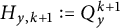 $H_{y,k+1}:=Q_y^{k+1}$
. By Lemma 2.6(1), we regard
 $U(t,\xi )$
as a lower solution of (1.3)–(1.6). Then,
 $$\begin{align*}U(0^+,\xi)\leq H_{0,k+1}^{m+1}[M]\leq H_{0,k+1}^{m}[M]\leq g(M)\leq M,\forall k\in\mathbb{N}.\end{align*}$$
Note that, if
 $a(\xi )$
is non-increasing in
 $\xi \in \mathbb {R}$
, then
 $g(a(\xi ))$
is also non-increasing, and thus
 $Q_y(a(\xi )) = P_y[g(a(\xi ))]$
is non-increasing in
 $\xi $
by the second property of [Reference Fang, Peng and Zhao10, Lemma 2.1]. Thus, there exists a non-increasing function
 $\phi (\xi )$
such that
 $H_{0,k+1}^{m}[M]$
converges locally uniformly to
 $\phi (\xi )$
. Hence,
 $H_{0,k+1}(\phi )=\phi $
. It follows from Lemma 2.6(2) that
 $$\begin{align*}\phi(+\infty)=\lim\limits_{y\to+\infty}\phi(y)=\lim\limits_{y\to+\infty}H_{0,k+1}(\phi)(y)=\lim\limits_{y\to+\infty}H_{y,k+1}[\phi(\cdot+y)](0).\end{align*}$$
Notice that
 $$ \begin{align*}\begin{aligned} &\lim\limits_{y\to+\infty}H_{y,k+1}[\phi(\cdot+y)](0)=\lim\limits_{y\to+\infty}U^y((k+1)T,0;\phi(\cdot+y))\\ &\qquad \qquad \qquad \qquad \qquad \quad =U^{+\infty}((k+1)T,0;\phi(+\infty))=H_{+\infty,k+1}(\phi({+\infty})). \end{aligned} \end{align*} $$
So,
 $\phi (+\infty )=H_{+\infty ,k+1}(\phi ({+\infty }))$
, similarly,
 $\phi (-\infty )=H_{-\infty ,k+1}(\phi ({-\infty }))$
. Observe that, (2.7) has only zero solution when
 $y=+\infty $
, and (2.7) has a zero solution or a T-periodic solution
 $p(t)$
when
 $y=-\infty $
(similar to the proof of [Reference Meng, Ge and Lin19, Theorem 3.4]), namely,
 $\phi (-\infty )=p(0)$
or
 $0$
,
 $\phi (+\infty )=0$
. By
 $\phi (\xi )\geq U(0^+,\xi )$
, we have
 $\phi (-\infty )=p(0)$
. By the comparison principle and
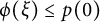 $\phi (\xi ) \leq p(0)$
, we conclude that
 $U(t,\xi ) \leq p(t)$
. Furthermore, the strong maximum principle implies that
 $U(t,\xi ) < p(t)$
. Moreover, due to
 $\phi (+\infty )=0$
, Lemma 2.6(2) implies
 $$\begin{align*}U(t,+\infty)=\lim\limits_{y\to+\infty}U(t,y;\phi(\cdot))=\lim\limits_{y\to+\infty}U^y(t,0;\phi(\cdot+y))=U^{+\infty}(t,0;\phi(+\infty))=0. \end{align*}$$
Then,
 $U(t,+\infty )=0$
uniformly in
 $[0,T]$
.
3 Propagation dynamics
Note that the analysis in this section is based on the assumptions (R), (G1)–(G4), and (H).
3.1 Forced KPP waves
We first use the monotonicity of
 $g(u)$
, combining with [Reference Meng, Ge and Lin19, Lemma 3.1], to derive the maximum principle and the comparison principle.
Lemma 3.1 (Maximum principle)
For any given
 $\phi (\xi )\geq 0$
, assume that, for some
 $c(t,\xi )\in L^\infty ([0,\infty )\times \mathbb {R})$
, function
 $U(t,\xi )\in C^{1,2}([0,\infty )\times \mathbb {R})$
satisfies
 $$ \begin{align*} \begin{cases} U_t\geq U_{\xi\xi}+cU_\xi+c(t,\xi)U,&t\in(kT^+,(k+1)T],\xi\in\mathbb{R},\\ U(kT^+,\xi)\geq g(U(kT,\xi)),&k\in\mathbb{N},\xi\in\mathbb{R},\\ U(0,\xi)=\phi(\xi)\geq 0,& \xi\in\mathbb{R}. \end{cases} \end{align*} $$
Then,
 $U(t,\xi ) \geq 0$
in
 $[0,\infty )\times \mathbb {R}$
. Moreover,
 $U(t,\xi )>0$
in
 $(0,\infty )\times \mathbb {R}$
if
 $\phi (\xi )\not \equiv 0$
in
 $\mathbb {R}$
.
Lemma 3.2 (Comparison principle)
Let
 $ U(t,\xi )$
be the unique solution of (1.3) and (1.4). Assume that there exists a function
 $\bar {U}(t,\xi )\in C^{1,2}([0,\infty )\times \mathbb {R})$
satisfying
 $$ \begin{align*} \begin{cases} \bar{U}_t\geq \bar{U}_{\xi\xi}+c\bar{U}_\xi+\bar{U}(r(t,\xi)-\bar{U}),&t\in(kT^+,(k+1)T],\xi\in\mathbb{R},\\ \bar{U}(kT^+,\xi)\geq g(\bar{U}(kT,\xi)),& k\in\mathbb{N},\xi\in\mathbb{R},\\ \bar{U}(0,\xi)\geq U(0,\xi),& \xi\in\mathbb{R}. \end{cases} \end{align*} $$
Then,
 $\bar {U}(t,\xi ) \geq U(t,\xi )$
in
 $[0,\infty )\times \mathbb {R}$
.
Recall that
 $c^*:=2\sqrt {\bar {r}(-\infty )+\frac {1}{T}\ln g'(0)}$
and
 $\bar {r}(\pm \infty )=\frac {1}{T}\int _0^T r(t,\pm \infty )dt$
, and
 $e^{\bar {r}(+\infty )}[g'(0)]^{\frac {1}{T}}<1<e^{\bar {r}(-\infty )}[g'(0)]^{\frac {1}{T}}$
. By a simple analysis, the equation
 $\mu ^2+c\mu +\bar {r}(+\infty )+\frac {1}{T}\ln g'(0)=0$
has a unique negative root
 $\mu _1<0$
for any given
 $c\in \mathbb {R}$
. If
 $c\geq c^*$
, then equation
 $\lambda ^2+c\lambda +\bar {r}(-\infty )+\frac {1}{T}\ln g'(0)=0$
admits two negative roots
 ${\lambda _1\leq \lambda _2<0}$
. Noting
 $\lambda _1^2+c\lambda _1+\bar {r}(+\infty )+\frac {1}{T}\ln g'(0)=\bar {r}(+\infty )-\bar {r}(-\infty )<0,$
we have
 $\lambda _1>\mu _1$
.
In this section, we discuss the existence/nonexistence of forced KPP waves for (1.2), which is equivalent to consider the properties of the solution to (1.3)–(1.6).
Theorem 3.3 The forced KPP wave of (1.2) exists only in the case that
 $c<c^*$
. Moreover, if it exists, denoted by
 $U(t,\xi )$
, then it is unique and non-increasing in
 $\xi \in \mathbb {R}$
.
Proof We divide the proof into three steps.
Step 1. We show that, if
 $c\geq c^*$
, no forced wave is present for (1.2). If system (1.3)–(1.6) has a positive T-periodic solution
 $U(t,\xi )$
for
 $c\geq c^*$
, then it follows from Lemma 2.7 that
 $U(t,\xi )<p(t)$
. We prove
 $U(t,-\infty )>p(t)$
to get a contradiction.
Claim:
 $U(t,\xi )=o(e^{(\mu _1+\eta )\xi })$
for some
 $\eta>0$
as
 $\xi \to +\infty $
. Letting
 $\epsilon _0=-\bar {r}(+\infty )>0$
, for any given
 $\epsilon \in (0,\epsilon _0)$
, there exists
 $\eta>0$
such that
 $\mu _1+\eta <0, \lambda _1\geq \mu _1+\eta ,$
and
 $$\begin{align*}(\mu_1+\eta)^2+c(\mu_1+\eta)+\bar{r}(+\infty)+\frac{1}{T}\ln g'(0)+\epsilon=0.\end{align*}$$
Choose
 $\xi _\epsilon>0$
satisfying
 $r(t,\xi )\leq r(t,+\infty )+\epsilon , \forall \xi \geq \xi _\epsilon .$
Define
 $$\begin{align*}\varphi_\epsilon(t)=e^{\int_0^t[(\mu_1+\eta)^2+c(\mu_1+\eta)+r(s,+\infty)+\frac{1}{T}\ln g'(0)+\epsilon]ds}, t\in (kT^+,(k+1)T], \text{ with }\varphi_\epsilon(kT)=[g'(0)]^{-1}.\end{align*}$$
Obviously,
 $\varphi _\epsilon (t+kT)=\varphi _\epsilon (t), \forall t\in (0^+,T]$
and
 $\varphi _\epsilon (kT^+)=g'(0)\varphi _\epsilon (kT)$
. Then, by the boundedness of
 $p(t)$
and
 $\varphi _\epsilon (t)$
, there is
 $M_\epsilon>0$
such that
 $$\begin{align*}M_\epsilon e^{(\mu_1+\eta)\xi}\varphi_\epsilon(t)\geq \max_{[0,T]}p(t), \forall \xi\leq \xi_\epsilon, t>0.\end{align*}$$
By
 $\mathbf {{(G2)}}$
,
 $g(u)\leq g'(0)u$
for
 $u>0$
. When
 $\xi>\xi _\epsilon $
, function
 $w_\epsilon (t,\xi ):=M_\epsilon e^{(\mu _1+\eta )\xi }\varphi _\epsilon (t)$
satisfies
 $$ \begin{align*} &(w_\epsilon)_t\kern1.4pt{-}\kern1.4pt(w_\epsilon)_{\xi\xi}\kern1.4pt{-}\kern1.4ptc(w_\epsilon)_\xi-w_\epsilon(r(t,\xi)-w_\epsilon)\kern1.4pt{=}\kern1.4pt[r(t,+\infty)+\epsilon-r(t,\xi)]w_\epsilon+(w_\epsilon)^2\kern1.4pt{\geq}\kern1.4pt 0,\\ &w_\epsilon(kT^+,\xi)=g'(0)w_\epsilon(kT,\xi)\geq g(w_\epsilon(kT,\xi)),k\in\mathbb{N}, \end{align*} $$
which means that
 $w(t,\xi ):=\min \{w_\epsilon (t,\xi ), p(t)\}$
is a generalized upper solution of system (1.3)–(1.6). The Claim holds if
 $w(t,\xi )\geq U(t,\xi )$
for
 $\xi \in \mathbb {R},t>0$
. Indeed,
 $w(t,\xi )\geq U(t,\xi )$
holds in
 $D:=\{(t,\xi )|w(t,\xi )\geq p(t)\}$
. If
 $(t,\xi )\not \in D$
, then
 $\xi>\xi _\epsilon $
. Define
 $$\begin{align*}\psi(t)=e^{\int_0^t [r(s,+\infty)+\epsilon_0]ds} \ \text{for} \ t\in (kT^+,(k+1)T] \ \text{with} \ \psi(kT)=[g'(0)]^{-1}.\end{align*}$$
There is
 $\delta>0$
such that
 $w(t,\xi )+\delta \psi (t)$
is also a generalized upper solution of system (1.3)–(1.6) for
 $(t,\xi )\not \in D$
. Due to
 $U(0,+\infty )=0$
, we can choose
 $\tau>0$
small enough such that
 $w(0,\xi )+\delta \psi (0)\geq \tau \geq U(0,\xi ), \forall \xi> \xi _\epsilon .$
Combining with
 $w(t,+\infty )+\delta \psi (t)=\delta \psi (t)>0=U(t,+\infty ),$
it deduces from the comparison principle that
 $w(t,\xi )+\delta \psi (t)\geq U(t,\xi )$
, and the strong maximum principle implies that
 $w(t,\xi )+\delta \psi (t)> U(t,\xi )$
. Letting
 $\delta \to 0$
, we have
 $w(t,\xi )\geq U(t,\xi )$
for
 $(t,\xi )\not \in D$
. Define
 $v^M(t,\xi ):=Me^{\lambda _1\xi }\chi (t)$
, where
 $$\begin{align*}\chi(t)=e^{\int_0^t [\lambda_1^2+c\lambda_1+r(t,-\infty)+\frac{1}{T}\ln g'(0)]ds} \ \text{for} \ t\in (kT^+,(k+1)T] \ \text{and} \ \chi(kT)=[g'(0)]^{-1}.\end{align*}$$
Similarly,
 $v^M(t,\xi )$
is also an upper solution of system (1.3)–(1.6) for some
 $M>0$
. By
 $\lambda _1\geq \mu _1+\eta $
and the Claim,
 $$\begin{align*}v^M(t,\xi)=Me^{\lambda_1\xi}\chi(t)\geq Me^{(\mu_1+\eta)\xi}\chi(t)= o(e^{(\mu_1+\eta)\xi})= U(t,\xi), \text{as} \ \xi\to \infty.\end{align*}$$
So we can find
 $M^*>0$
and
 $\xi (t)\in \mathbb {R}$
satisfying
 $v^{M^*}(t,\xi )\geq U(t,\xi ),\forall t>0,\xi \in \mathbb {R}$
and
 $ v^{M^*}(t,\xi (t))= U(t,\xi (t)).$
Thus,
 $W(t,\xi ):=v^{M^*}(t,\xi )-U(t,\xi )$
satisfies
 $W(t,\xi )\geq 0$
and
 $W(t,\xi (t))=0$
for any
 $ t>0,\xi \in \mathbb {R}$
. Observing that
 $$\begin{align*}W_t-W_{\xi\xi}-cW_\xi-r(t,-\infty)W=[r(t,-\infty)-r(t,\xi)]W+W^2\geq0,\end{align*}$$
the strong maximum principle implies that
 $v^{M^*}(t,\xi )\equiv U(t,\xi )$
, then
 $v^{M^*}(t,-\infty )=+\infty $
. This is a contradiction with
 $U(t,\xi )<p(t)$
. Then, Step 1 is compete.
Step 2. We show that, if there is a forced KPP wave for (1.2), then it is unique. Assume that system (1.3)–(1.6) has two different positive solutions
 $U_i(t,\xi )(i=1,2)$
. Clearly,
 $0<U_i(t,\xi )<p(t)$
,
 $U_i(t,+\infty )=0,$
and
 $U_i(t,-\infty )=p(t)$
. For any
 $\epsilon>0$
, define
 $$\begin{align*}K_\epsilon:=\{k\geq1|kU_1(t,\xi)\geq U_2(t,\xi)-\epsilon q(t,\xi)\},\end{align*}$$
where
 $q(t,\xi )$
is a positive, continuous, and bounded T-periodic function satisfying
 $q(t,\pm \infty )>\delta >0$
for some
 $\delta>0$
. Notice that
 $$\begin{align*}&\lim\limits_{\xi\to-\infty}\dfrac{U_2(t,\xi)-\epsilon q(t,\xi)}{U_1(t,\xi)}\\&\quad=\dfrac{p(t)-\epsilon q(t,-\infty)}{p(t)}, \lim\limits_{\xi\to+\infty}\dfrac{U_2(t,\xi)-\epsilon q(t,\xi)}{U_1(t,\xi)}=-\infty \ \text{uniformly in} \ [0,T].\end{align*}$$
Thus, there is
 $L_\epsilon>0$
such that
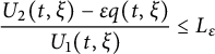 $\dfrac {U_2(t,\xi )-\epsilon q(t,\xi )}{U_1(t,\xi )}\leq L_\epsilon $
on
 $[0,T]\times \mathbb {R}$
, namely,
 ${K_\epsilon \neq \emptyset} $
. Denote
 $k_\epsilon :=\inf K_\epsilon \text { and } k^*:=\lim \limits _{\epsilon \to 0}k_\epsilon $
. So,
 $k_\epsilon U_1(t,\xi )\geq U_2(t,\xi )-\epsilon q(t,\xi )$
and
 $k_\epsilon $
is non-increasing in
 $\epsilon>0$
and
 $k^*\geq 1$
. In the following, we shall show
 $k^*=1$
. By way of contradiction, if
 $k^*>1$
, then there exists
 $\epsilon _0>0$
such that
 $k_{\epsilon _0}>1$
and
 $k_\epsilon \geq k_{\epsilon _0}>1$
for any
 $0<\epsilon <\epsilon _0$
. Define
 $$ \begin{align*} &w_\epsilon(t,\xi):=k_\epsilon U_1(t,\xi)- U_2(t,\xi)+\epsilon q(t,\xi)\geq 0;\\ &w(t,\xi):=\lim\limits_{\epsilon\to0}w_\epsilon(t,\xi)=k^*U_1(t,\xi)- U_2(t,\xi). \end{align*} $$
There exists
 $(t_\epsilon ,\xi _\epsilon )$
such that
 $w_\epsilon (t_\epsilon ,\xi _\epsilon )=0$
and
 $w_\epsilon (t,\xi )>0$
in any neighborhood of
 $(t_\epsilon ,\xi _\epsilon )$
. Indeed, if
 $w_\epsilon (t,\xi )>0$
for
 $t>0$
and
 $\xi \in \mathbb {R}$
, then for such
 $\epsilon $
, we can find
 $\eta>0$
small enough such that
 $k_\epsilon -\eta>1$
and
 $\frac {w_\epsilon (t,\xi )}{U_1(t,\xi )}\geq \eta $
, which means
 $(k_\epsilon -\eta )U_1(t,\xi )- U_2(t,\xi )+\epsilon q(t,\xi )\geq 0.$
This contradicts the definition of
 $k_\epsilon $
. We consider three different possibilities for
 $\{\xi _\epsilon \}$
: (i)
 $\{\xi _\epsilon \}$
is bounded; (ii)
 $\{\xi _\epsilon \}\nearrow +\infty $
as
 $\epsilon \to 0$
; and (iii)
 $\{\xi _\epsilon \}\searrow -\infty $
as
 $\epsilon \to 0$
.
For case (i), if
 $\{\xi _\epsilon \}$
is bounded, then
 $k^*<+\infty $
and there is
 $(t^*,\xi ^*)\in \mathbb {R}^+\times \mathbb {R}$
such that
 $\{(t_\epsilon ,\xi _\epsilon )\}\to (t^*,\xi ^*)$
as
 $\epsilon \to 0$
and
 $w(t^*,\xi ^*)=0$
. Note that
 $$ \begin{align*} &w_t-w_{\xi\xi}-cw_\xi\geq r(t,\xi)w+U_2^2-(k^*U_1)^2=[r(t,\xi)-k^*U_1-U_2]w;\\ &w(kT^+,\xi)\kern1.4pt{=}\kern1.4pt k^*g(U_1(kT,\xi))\kern1.4pt{-}\kern1.4pt g(U_2(kT,\xi))\kern1.4pt{\geq}\kern1.4pt g(k^*U_1(kT,\xi))\kern1.4pt{-}\kern1.4pt g(U_2(kT,\xi))\kern1.4pt{\geq}\kern1.4pt 0. \end{align*} $$
By the strong maximum principle, it follows from
 $w(t,\xi )\geq 0$
and
 $w(t^*,\xi ^*)=0$
that
 $w(t,\xi )\equiv 0$
on
 $[0,T]\times \mathbb {R}$
, which contradicts
 $w(t,-\infty )=(k^*-1)p(t)>0$
. For case (ii), if
 $\{\xi _\epsilon \}\nearrow +\infty $
as
 $\epsilon \to 0$
, then
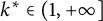 $k^*\in (1,+\infty ]$
. Choose
 $\delta _\epsilon>0$
such that
 $$ \begin{align*} (w_\epsilon)_t&=k_\epsilon(U_1)_t-(U_2)_t+\epsilon q_t\\ &=(w_\epsilon)_{\xi\xi}+c(w_\epsilon)_\xi+k_\epsilon U_1[r(t,\xi)-U_1]- U_2[r(t,\xi)-U_2]+\epsilon[q_t-q_{xx}-cq_x]\\ &\geq [r(t,\xi)-k_\epsilon U_1-U_2](k_\epsilon U_1-U_2)+\epsilon[q_t-q_{xx}-cq_x]\\ &=[r(t,\xi)-k_\epsilon U_1-U_2]w_\epsilon+\epsilon[q_t-q_{\xi\xi}-cq_\xi-(r(t,\xi)-k_\epsilon U_1-U_2)q] \end{align*} $$
in domain
 $Q_\epsilon =[0,T]\times (\xi _\epsilon -\delta _\epsilon ,\xi _\epsilon +\delta _\epsilon )$
. We find that, if
 $$ \begin{align} q_t-q_{\xi\xi}-cq_\xi-(r(t,\xi)-k_\epsilon U_1-U_2)q\geq0, (t,\xi)\in Q_\epsilon, \end{align} $$
then it follows from
 $w_\epsilon \geq 0$
and the strong maximum principle that
 $w_\epsilon \equiv 0$
in
 $Q_\epsilon $
, a contradiction with the definition of
 $(t_\epsilon ,x_\epsilon )$
. For case (iii), if
 $\{\xi _\epsilon \}\searrow -\infty $
as
 ${\epsilon \to 0}$
, then
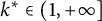 $k^*\in (1,+\infty ]$
and
 $ (w_\epsilon )_t-(w_\epsilon )_{\xi \xi }-c(w_\epsilon )_\xi -[r(t,\xi )-k_\epsilon U_1-U_2]w_\epsilon \geq 0 $
in domain
 $Q_\epsilon $
if (3.1) holds in
 $Q_\epsilon $
. Similarly, the strong maximum principle deduces a contradiction. In what follows, we construct
 $q(t,\xi )$
satisfying (3.1) in
 $Q_\epsilon $
. For any
 $t>0$
,
 $$\begin{align*}&\lim\limits_{\xi\to+\infty}[r(t,\xi)-k_\epsilon U_1-U_2]\\&\quad=r(t,+\infty); \lim\limits_{\xi\to-\infty}[r(t,\xi)-k_\epsilon U_1-U_2]=r(t,-\infty)-(k_\epsilon+1)p(t). \end{align*}$$
Then, there is
 $x_+>0$
satisfying
 $r(t,\xi )-k_\epsilon U_1-U_2\leq r(t,+\infty )-\bar {r}(+\infty ):=\alpha _1(t), \xi \geq x_+$
and there is
 $x_-<0$
satisfying
 $$\begin{align*}r(t,\xi)-k_\epsilon U_1-U_2\leq r(t,-\infty)-(k_\epsilon+1)p(t)+\frac{1}{k_\epsilon}\frac{1}{T}\int_0^Tp(t)dt:=\alpha_2(t), \xi\leq x_-.\end{align*}$$
Noting that
 $\alpha _1(t),\alpha _2(t)$
are T-periodic function, we choose
 $q(t,\xi )\in C^{1,1}([0,T],\mathbb {R})$
such that
 $q(t,\xi )=e^{\int _0^t\alpha _1(s)ds}$
for
 $\xi \geq x_+$
,
 $q(t,\xi )=e^{\int _0^t\alpha _2(s)ds}$
for
 $\xi \leq x_-$
, and
 $0\leq q(t,\xi )\leq e^{\int _0^t\alpha _1(s)ds}$
for
 $0\leq \xi \leq x_+$
,
 $0\leq q(t,\xi )\leq e^{\int _0^t\alpha _2(s)ds}$
for
 $x_-\leq \xi \leq 0$
. Then, (3.1) holds for
 $\xi \leq x_-$
and
 $\xi \geq x_+$
, completing the proof of Step 2.
Step 3. We show that, for
 $c<c^*$
, system (1.2) has a forced KPP wave
 $U(t,\xi )$
non-increasing in
 $\xi \in \mathbb {R}$
. To establish the existence of solutions to the system (1.3)–(1.6), we show that there exists a function
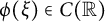 $\phi (\xi ) \in C(\mathbb {R})$
satisfying (1.3)–(1.5) and the boundary conditions
 $$\begin{align*}U(0,+\infty)=\phi(+\infty)=0,U(0,-\infty)=\phi(-\infty)=p(0).\end{align*}$$
From Lemma 2.7, there exists a non-increasing function
 $\phi (\xi )$
such that
 $H_{0,k+1}^{m}[M]$
converges locally uniformly to
 $\phi (\xi )$
and satisfies
 $H_{0,k+1}(\phi )=\phi $
, where
 $\phi (+\infty )$
equals
 $0$
and
 $\phi (-\infty )$
equals either
 $p(0)$
or
 $0$
. Notably, if
 $\phi (-\infty )=p(0)$
, then
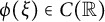 $\phi (\xi ) \in C(\mathbb {R})$
satisfies (1.3)–(1.5) and the boundary conditions (1.6) for
 $t=0$
. Furthermore,
 $U(t,\xi )$
is non-increasing in
 $\xi \in \mathbb {R}$
since the initial value
 $\phi (\xi )$
is non-increasing in
 $\xi \in \mathbb {R}$
. If system (1.3)–(1.6) admits a solution
 $U\geq $
and
 $\not \equiv 0$
, then it follows that
 $\phi (-\infty )=p(0)$
. It suffices to show that U is nonnegative and not identically zero. Namely, we need to construct a nonnegative, nonzero lower solution for system (1.3)–(1.6).
We consider (i)
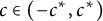 $c\in (-c^*,c^*)$
and (ii)
 $c\leq -c^*$
. For case (i), for given
 $M,L>0$
, let
 $(\nu _1,\psi (\xi )$
be the principal eigen-pair of
 $$\begin{align*}\psi"(\xi)-\frac{1}{T}\ln g'(0)\psi(\xi)=\nu\psi(\xi), \xi\in [-M-L,-M] \text{ with }\psi(-M-L)=\psi(-M)=0.\end{align*}$$
Clearly,
 $\nu _1=-\frac {1}{T}\ln g'(0)-(\frac {\pi }{L})^2$
. It follows from (H) that there exists
 $L_0>0$
such that
 $\nu _1\geq 0$
for
 $L\geq L_0$
. Meanwhile, we extend
 $\psi (\xi )$
to
 $\mathbb {R}$
by letting
 $\psi (\xi )=0$
for
 $\xi \not \in [-M-L,-M]$
. Define
 $$\begin{align*}\varphi(t):=e^{\int_0^t[r(t,-\infty)+\frac{1}{T}\ln g'(0)-\frac{(c^*)^2}{4}]ds},t\in (kT^+,(k+1)T] \text{ with } \varphi(kT)=[g'(0)]^{-1}.\end{align*}$$
It is easy to see that
 $\varphi (t+kT)=\varphi (t)$
for any
 $t\in (0^+,T]$
,
 $\varphi (kT^+)=g'(0)\varphi (kT)$
. Now, we construct a lower solution of (1.3)–(1.6):
 $$ \begin{align} \underline{U}(t,\xi):= \begin{cases} \epsilon_0e^{\gamma(t-kT)-\frac{c}{2}\xi}\psi(\xi)\varphi(t),& t\in (kT^+,(k+1)T],\xi\in\mathbb{R},\\ \epsilon_0e^{-\frac{c}{2}\xi}\psi(\xi)\varphi(kT^+),& t=kT^+,\xi\in\mathbb{R},\\ \epsilon_0e^{\gamma T-\frac{c}{2}\xi}\psi(\xi)\varphi(kT),& t=kT,\xi\in\mathbb{R}, \end{cases} \end{align} $$
where
 $\epsilon _0>0$
is sufficiently small and
 $\gamma>0$
will be determined later. Notice that for
 $\epsilon>0$
, there are
 $\delta _\epsilon>0$
and
 $\xi _\epsilon <0$
satisfying
 $$ \begin{align} r(t,\xi)-U(t,\xi)\geq r(t,-\infty)-\epsilon, \text{for} \ U\in[0,\delta_\epsilon],\xi\leq \xi_\epsilon. \end{align} $$
Then,
 $$ \begin{align*} &\underline{U}_t - \underline{U}_{\xi\xi} - c\underline{U}_\xi - \underline{U}[r(t,\xi) - \underline{U}] \\&\quad= \left(\gamma + \varphi'(t)/\varphi(t)\right)\underline{U} + (c^2/4)\underline{U} - \left(\nu_1 + (1/T)\ln g'(0)\right)\underline{U} - \underline{U}[r(t,\xi) - \underline{U}] \\ &\quad\leq \Big[\gamma + c^2/4 - \nu_1 - (1/T)\ln g'(0) + \varphi'(t)/\varphi(t) - r(t,-\infty) + \epsilon\Big]\underline{U} \\ &\quad= \Big[\gamma + c^2/4 - \nu_1 - (c^*)^2/4 + \epsilon\Big]\underline{U} \end{align*} $$
provided that
 $0\leq \underline {U}\leq \delta _\epsilon $
for
 $\xi \leq \xi _\epsilon $
. Since
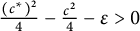 $\frac {(c^*)^2}{4}-\frac {c^2}{4}-\epsilon>0$
for
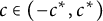 $c\in (-c^*,c^*)$
and small
 $\epsilon>0$
, together with
 $\nu _1\geq 0$
for
 $L\geq L_0$
, we observe that
 $\gamma :=-\frac {c^2}{4}+\nu _1+\frac {(c^*)^2}{4}-\epsilon>0$
for
 $L\geq L_0$
and small
 $\epsilon $
. Thus,
 $\underline {U}_t-\underline {U}_{\xi \xi }-c\underline {U}_\xi -\underline {U}[r(t,\xi )-\underline {U}]\leq 0.$
Moreover, we apply
 $\mathbf {{(G4)}}$
and
 $\gamma>0$
to obtain
 $$ \begin{align*} \underline{U}(kT^+,\xi)-g(\underline{U}(kT,\xi))&\leq \underline{U}(kT^+,\xi)-g'(0)\underline{U}(kT,\xi)+D\underline{U}^\rho(kT,\xi)\\ &=\epsilon_0e^{-\frac{c}{2}\xi}\psi(\xi)-\epsilon_0e^{\gamma T-\frac{c}{2}\xi}\psi(\xi)+D\epsilon_0^\rho e^{\gamma T\rho-\frac{c}{2}\xi\rho}\psi^\rho(\xi)(g'(0))^{-\rho}\\ &=\epsilon_0e^{-\frac{c}{2}\xi}\psi(\xi)[1-e^{\gamma T}+D\epsilon_0^{\rho-1} e^{\gamma T\rho-\frac{c}{2}\xi(\rho-1)}\psi^{\rho-1}(\xi)(g'(0))^{-\rho}]\leq0, \end{align*} $$
if
 $\epsilon _0$
is sufficiently small. The comparison principle implies that
 $\underline {U}$
is a nonnegative lower solution if
 $0\leq \underline {U}\leq \delta _\epsilon $
for
 $\xi \leq \xi _\epsilon $
. Indeed,
 $ \sup _{(t,\xi )\in (0,+\infty )\times (\xi _\epsilon -L,\xi _\epsilon )}\underline {U}(t,\xi )\leq \epsilon _0e^{\gamma T}e^{-\frac {c}{2}(\xi _\epsilon -L)}\max _{[0,T]}\varphi (t). $
As long as
 $\epsilon _0\leq [e^{\gamma T}e^{-\frac {c}{2}(\xi _\epsilon -L)}\max _{[0,T]}\varphi (t)]^{-1} \delta _\epsilon ,$
it deduces that
 $0\leq \underline {U}\leq \delta _\epsilon $
for
 $\xi \leq \xi _\epsilon $
. Take
 $M=-\xi _\epsilon $
and
 $L=L_0$
, then the conclusion holds for
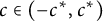 $c\in (-c^*,c^*)$
. For case (ii), for such
 $\epsilon>0$
given by (3.3), it follows from
 ${c\leq -c^*}$
and
 $\bar {r}(-\infty )-\epsilon>0$
that
 $\mu _2>0$
is the smaller positive root of
 $\mu ^2+c\mu +\bar {r}(-\infty )-\epsilon =0.$
Then, there is
 $\eta>0$
small enough such that
 $(\mu _2+\eta )^2+c(\mu _2+\eta )+\bar {r}(-\infty )-\epsilon <0.$
For such a given
 $\eta>0$
, choosing
 $M>1$
, there is
 $\xi _M<0$
such that
 $1=Me^{\eta \xi _M}$
. Define
 $$ \begin{align*} \underline{U}(t,\xi):= \begin{cases} 0,& t>0,\xi\geq\xi_M,\\ \epsilon_0 \beta(t)[e^{\mu_2\xi}-Me^{(\mu_2+\eta)\xi}] ,& t\in (kT^+,(k+1)T],\xi\leq\xi_M,\\ \epsilon_0\beta(kT^+)[e^{\mu_2\xi}-Me^{(\mu_2+\eta)\xi}],& t=kT^+,\xi\leq\xi_M,\\ \epsilon_0\beta(kT)e^{\mu_2 T}[e^{\mu_2\xi}-Me^{(\mu_2+\eta)\xi}],& t=kT,\xi\leq\xi_M,\\ \end{cases} \end{align*} $$
where
 $\epsilon _0>0$
is small enough and
 $\beta (t)$
satisfies
 $$\begin{align*}\beta(t):=e^{\int_0^t[\mu_2^2+c\mu_2+r(t,-\infty)-\epsilon]ds},t\in (kT^+,(k+1)T] \text{ with }\beta(kT)=[g'(0)]^{-1}.\end{align*}$$
Note that
 $$\begin{align*}\sup_{(t,\xi)\in(0,+\infty)\times(-\infty,\xi_M)}\underline{U}(t,\xi)\leq \epsilon_0e^{\mu_2\xi_M}e^{\mu_2 T}\max_{[0,T]}\beta(t)\leq \delta_\epsilon \end{align*}$$
for
 $\epsilon _0>0$
sufficiently small. Then,
 $$ \begin{align*} &\quad\underline{U}_t-\underline{U}_{\xi\xi}-c\underline{U}_\xi-\underline{U}[r(t,\xi)-\underline{U}]\\ &=\epsilon_0 \beta(t)e^{\mu_2\xi}[\frac{\beta'(t)}{\beta(t)}-\mu_2^2-c\mu_2]\\&\qquad-\epsilon_0 \beta(t)Me^{(\mu_2+\eta)\xi}[\frac{\beta'(t)}{\beta(t)}-(\mu_2+\eta)^2-c(\mu_2+\eta)]-\underline{U}[r(t,\xi)-\underline{U}]\\ &\leq \epsilon_0 \beta(t)e^{\mu_2\xi}[\frac{\beta'(t)}{\beta(t)}-\mu_2^2-c\mu_2-r(t,-\infty)+\epsilon]\\ &\quad\quad-\epsilon_0 \beta(t)Me^{(\mu_2+\eta)\xi}[\frac{\beta'(t)}{\beta(t)}-(\mu_2+\eta)^2-c(\mu_2+\eta)-r(t,-\infty)+\epsilon]<0 \end{align*} $$
and
 $$ \begin{align*} &\underline{U}(kT^+,\xi)-g(\underline{U}(kT,\xi))\leq \underline{U}(kT^+,\xi)-g'(0)\underline{U}(kT,\xi)+D\underline{U}^\rho(kT,\xi)\\ &\quad=\epsilon_0[e^{\mu_2\xi}-Me^{(\mu_2+\eta)\xi}][1-e^{\mu_2 T}+D\epsilon_0^{\rho-1} e^{\mu_2 T\rho}\beta^{\rho-1}(\xi)(g'(0))^{-\rho}]\leq0. \end{align*} $$
Thus, the conclusion holds for
 $c\leq -c^*$
. We have constructed a nonnegative lower solution that is nonzero for system (1.3)–(1.6), and Step 3 is proved. Thus, the theorem holds.
3.2 Spreading properties
Denote by
 $u(t,x;u_0)$
the solution of (1.2) for a given
 $u_0 \in C(\mathbb {R},\mathbb {R}^+)$
. We can also utilize the monotonicity of
 $g(u)$
to derive the comparison principle.
Lemma 3.4 (Comparison principle)
If there exists a function
 $\bar {u}(t,\xi )\in C^{1,2}([0,\infty )\times \mathbb {R})$
satisfying
 $$ \begin{align*} \begin{cases} \bar{u}_t\geq\bar{u}_{xx}+\bar{u}(r(t,x-ct)-\bar{u}),&t\in(kT^+,(k+1)T],x\in\mathbb{R},\\ \bar{u}(kT^+,x)\geq g(\bar{u}(kT,x)),&x\in\mathbb{R},k\in\mathbb{N},\\ \bar{u}(0,x)\geq u_0(x),&x\in\mathbb{R}, \end{cases} \end{align*} $$
then
 $\bar {u}(t,x) \geq u(t,x)$
in
 $[0,\infty )\times \mathbb {R}$
.
In this section, we study the long-time behavior for (1.2) with different c. For
 $c < c^*$
, by Theorem 3.3, system (1.2) admits a forced KPP wave
 $U(t,x-ct)$
. Now, we demonstrate that the solution of (1.2) with sufficiently large initial data
 $M \geq p(0)$
, denoted by
 $u(t,x;M)$
, uniformly converges to the forced KPP wave as
 $t \to +\infty $
.
Lemma 3.5 For
 $c<c^*$
, choosing
 $M\geq p(0)$
,
 $$ \begin{align} \lim\limits_{t\to+\infty}|u(t,x;M)-U(t,x-ct)|=0, \end{align} $$
uniformly in
 $\mathbb {R}$
.
Proof By the proof of Lemma 2.7, there exists a non-increasing
 $\phi (\xi )$
satisfying
 $\phi (+\infty )=0$
and
 $\phi (-\infty )=p(0)$
such that
 $H_{0,k+1}^{m}[M]$
converges locally uniformly to
 $\phi (\xi )$
for
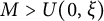 $M>U(0,\xi )$
. This implies that, for any bounded set
 $[-L,x_0]$
of
 $\mathbb {R}$
, equation (3.4) holds uniformly in
 $x-ct\in [-L,x_0]$
. Choose L large enough, it then follows that
 $\lim \limits _{t\to +\infty }|p(t)-U(t,x-ct)|=0 \ \text {uniformly in} \ x-ct\leq -L.$
Note that the unique positive solution
 $\alpha (t;M)$
of (2.1) with
 $u_0=M$
satisfies
 $\lim \limits _{t\to +\infty }|p(t)-\alpha (t;M)|=0$
from Lemma 2.1 and is an upper solution of (1.2) with initial value M due to
 $r(t,\xi )\leq r(t,-\infty )$
. In view of
 $U(0,\xi )\leq U(0,-\infty )=p(0)\leq M$
, the comparison principle implies that
 $U(t,\xi )\leq u(t,x;M)\leq \alpha (t;M)$
. This deduces that
 $$ \begin{align*} &\limsup\limits_{t\to+\infty}[u(t,x;M)-U(t,x-ct)]\leq \limsup\limits_{t\to+\infty}[\alpha(t;M)-U(t,x-ct)]\\ &\quad\leq \lim\limits_{t\to+\infty}|\alpha(t;M)-p(t)|+\limsup\limits_{t\to+\infty}|p(t)-U(t,x-ct)|=0 \end{align*} $$
uniformly in
 $x-ct\leq -L$
. Combining with
 $\limsup \limits _{t\to +\infty }[u(t,x;M)-U(t,x-ct)]\geq 0$
, equation (3.4) holds uniformly in
 $x-ct\leq -L$
. For
 $x-ct> x_0$
, assume that there are
 $\delta _0>0$
and
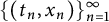 $\{(t_n,x_n)\}_{n=1}^\infty $
satisfying
 $x_n-ct_n\to +\infty $
such that
 $u(t_n,x_n;M)=\delta _0$
. Obviously, there is
 $t_*\in (0,T]$
such that
 $\lim \limits _{n\to +\infty }t_n-[t_n/T]T=t_*,$
where
 $[t_n/T]$
is the inter part of
 $t_n/T$
. Let
 $w_n(t,x):=u(t+t_n,x+x_n;M)$
. We can find a function w such that
 $w_n\to w$
locally uniformly holds as
 $n\to \infty $
, and w satisfies
 $$ \begin{align*} \begin{cases} w_t=w_{xx}+w(r(t+t_*,+\infty)-w),&t\in(kT^+,(k+1)T],x\in\mathbb{R},\\ w(kT^+-t_*,x)=g(w(kT-t_*,x)),&x\in\mathbb{R},k\in\mathbb{N},\\ u(0,x)=M,&x\in\mathbb{R} \end{cases} \end{align*} $$
and
 $w(0,0)=\lim \limits _{n\to +\infty }w_n(0,0)=\delta _0>0.$
By Remark 2.2,
 $w\equiv 0$
, which is a contradiction. Thus, equation (3.4) holds uniformly in
 $x-ct\geq x_0.$
The proof is complete.
Meanwhile, for
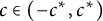
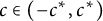 $c\in (-c^*,c^*)$
, we shall construct a pair of upper–lower solutions of (1.2) by using the forced wave.
Lemma 3.6 Function
 $w^{\pm }(t,x)=U(t,x-ct)\pm \rho e^{-\sigma (t-\xi _0)}[1+M U(t,x-ct)]$
is a pair of upper and lower solutions of (1.2), where
 $\xi _0\in \mathbb {R}$
,
 $\sigma>0$
small enough,
 $\rho>0$
, and M large enough will be determined later.
Proof We only show that
 $w^{+}$
is an upper solution of (1.2). Note that
 $$ \begin{align*} &w^{+}_t(t,x)=U_t(t,x-ct)-cU_\xi(t,x-ct)-\sigma\rho e^{-\sigma(t-\xi_0)}[1+M U(t,x-ct)]\\ &\quad\quad\quad\quad+\rho e^{-\sigma(t-\xi_0)}M[U_t(t,x-ct)-cU_\xi(t,x-ct)];\\ &w^{+}_{xx}(t,x)=U_{\xi\xi}(t,x-ct)+\rho e^{-\sigma(t-\xi_0)}MU_{\xi\xi}(t,x-ct). \end{align*} $$
Then,
 $$ \begin{align*} &w^{+}_t-w^{+}_{xx}(t,x)-w^{+}(r(t,x-ct)-w^{+})\\ =&\ \rho e^{-\sigma(t-\xi_0)}\{(1+M U(t,x-ct))[-\sigma+(1+M U(t,x-ct))e^{-\sigma(t-\xi_0)}]\\ &-r(t,x-ct)+2U(t,x-ct)+MU^2(t,x-ct)\}. \end{align*} $$
The properties of
 $U(t,x-ct)$
and
 $r(t,\xi )$
mean that, there exist
 $\sigma>0$
small enough and M large enough satisfying
 $$ \begin{align*} &(1+M U(t,x-ct))e^{-\sigma(t-\xi_0)}>\sigma;\\ &-r(t,x-ct)+2U(t,x-ct)+MU^2(t,x-ct)>0;\\ &\rho e^{-\sigma(kT-\xi_0)}(1+M U(kT,x-ckT))>N,\rho e^{-\sigma(kT-\xi_0)}M>1, \end{align*} $$
where N is given by
 $\textbf {(G3)}$
. Hence,
 $w^{+}_t-w^{+}_{xx}(t,x)-w^{+}(r(t,x-ct)-w^{+})\geq 0.$
Meanwhile, it follows from
 $\textbf {(G2)}$
and
 $\textbf {(G3)}$
that
 $$\begin{align*}g(\rho e^{-\sigma(kT-\xi_0)}Mu)\leq \rho e^{-\sigma(kT-\xi_0)}Mg(u), \forall u>0\end{align*}$$
and
 $$\begin{align*}\frac{g(\rho e^{-\sigma(kT-\xi_0)}(1+MU(kT,x-ckT)))}{\rho e^{-\sigma(kT-\xi_0)}(1+MU(kT,x-ckT))}<1.\end{align*}$$
Consequently,
 $$ \begin{align*} w^{+}(kT^+,x)&=g(U(kT,x-ckT))+\rho e^{-\sigma(kT-\xi_0)}+\rho e^{-\sigma(kT-\xi_0)}Mg(U(kT,x-ckT))\\ &\geq g(U(kT,x-ckT))+\rho e^{-\sigma(kT-\xi_0)}+g(\rho e^{-\sigma(kT-\xi_0)}MU(kT,x-ckT))\\ &\geq g(U(kT,x-ckT))+\rho e^{-\sigma(kT-\xi_0)}\\ &\quad+[1-\frac{1}{1+MU(kT,x-ckT)}] g(\rho e^{-\sigma(kT-\xi_0)}(1+MU(kT,x-ckT)))\\ &\geq g(U(kT,x-ckT))+g(\rho e^{-\sigma(kT-\xi_0)}(1+MU(kT,x-ckT)))\\ &\quad+\rho e^{-\sigma(kT-\xi_0)}[1-\frac{g(\rho e^{-\sigma(kT-\xi_0)}(1+MU(kT,x-ckT)))}{\rho e^{-\sigma(kT-\xi_0)}(1+MU(kT,x-ckT))}]\\ &\geq g(U(kT,x-ckT))+g(\rho e^{-\sigma(kT-\xi_0)}(1+MU(kT,x-ckT)))\\ &\geq g(U(kT,x-ckT)+\rho e^{-\sigma(kT-\xi_0)}(1+MU(kT,x-ckT)))=g(w^+). \end{align*} $$
Thus,
 $w^{+}$
is an upper solution of (1.2).
Then, by Lemmas 3.5 and 3.6, we obtain the spreading properties of solution of (1.2).
Theorem 3.7 Denote by
 $u(t,x;u_0)$
the solution of (1.2), where
 $u_0(x)\geq $
but
 $\not \equiv 0$
is bounded.
-
(1) For
$c\leq -c^*$
, if further
$u_0(x)$
has a compact support, then
$$\begin{align*}\limsup\limits_{m\to+\infty} u(t+mT,x;u_0)=0, \ \text{uniformly in} \ [0,T]\times\mathbb{R}.\end{align*}$$
-
(2) For
$c\in (-c^*,c^*)$
, (3.5)
$$ \begin{align} \lim\limits_{t\to+\infty}\sup_{x\geq-\mu t} |u(t,x;u_0)-U(t,x-ct)|=0 \ \text{for any} \ \mu\in(c,c^*). \end{align} $$
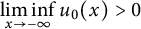
Moreover, if
$\liminf \limits _{x\to -\infty } u_0(x)>0$
, then there is
$\mu>0$
such that (3.6)
$$ \begin{align} \lim\limits_{t\to+\infty}\sup_{x\in \mathbb{R}} |u(t,x;u_0)-U(t,x-ct)|e^{\mu t}=0. \end{align} $$





Proof (1) Define two operators:
 $$ \begin{align*} &L\phi(x):=\phi"(x)+c\phi'(x)+\bar{r}(-\infty)\phi(x),,x\in\mathbb{R}; \\ &\tilde{L}_t\phi(x):=\phi"(x)+c\phi'(x)+r(t,-\infty)\phi(x),x\in\mathbb{R}. \end{align*} $$
Observe from [Reference Wang and Wang37, Section 2] and [Reference Berestycki and Rossi7, Proposition 2] that the eigenvalue equation
 ${-L\phi =\lambda \phi ,x\in \mathbb {R}}$
has a principle eigenvalue
 $\lambda (-L):=-\bar {r}(-\infty )+\frac {c^2}{4}$
and there is a positive eigenfunction
 $\phi ^*(x)$
with
 $\|\phi ^*\|_\infty =1$
such that
 $-L\phi ^*=\lambda (-L)\phi ^*$
. Since
 $r(t,-\infty )$
is a T-periodic function in t, the eigenvalue equation
 $-\tilde {L}_t\phi =\lambda \phi ,x\in \mathbb {R}$
also has a principle eigenvalue
 ${\lambda }(-\tilde {L}_t)=\lambda (-L)$
. Referring to [Reference Wu and Zhao39, Section 2.1], we discuss the following linear model:
 $$ \begin{align*} \begin{cases} w^{(m)}_t=w^{(m)}_{xx}+cw^{(m)}_x+r(t,-\infty)w^{(m)},&t\in(0^+,T],x\in\mathbb{R},\\ w^{(m)}(0^+,x)=g'(0)w^{(m)}(0,x),&x\in\mathbb{R},\\ w^{(m)}(0,x)=w^{(m-1)}(T,x),&x\in\mathbb{R}, \end{cases} \end{align*} $$
with
 $w^{(0)}(0,x)=M\phi ^*(x)$
. It follows easily that
 $w^{(m)}(t,x)=M(e^{-\lambda (-\tilde {L}_t)T}g'(0))^me^{-\lambda (-\tilde {L}_t)t}g'(0)\phi ^*(x). $
Note that, for
 $c\leq -c^*$
,
 $$\begin{align*}-\lambda(-\tilde{L}_t)T+\ln g'(0)=[\bar{r}(-\infty)-\frac{c^2}{4}+\frac{1}{T}\ln g'(0)]T=[\frac{(c^*)^2}{4}-\frac{c^2}{4}]T\leq0. \end{align*}$$
Then,
 $\tilde {w}^{(m)}(t,x):=w^{(m)}(t,x-ct)$
satisfies
 $$\begin{align*}\tilde{w}^{(m)}(t,x)=M(e^{-\lambda(-\tilde{L}_t)T}g'(0))^me^{-\lambda(-\tilde{L}_t)t}g'(0)\phi^*(x-ct)\to 0, \text{ as }m\to+\infty\end{align*}$$
and
 $$ \begin{align*} \begin{cases} \tilde{w}^{(m)}_t=\tilde{w}^{(m)}_{xx}+r(t,-\infty)\tilde{w}^{(m)},&t\in(0^+,T],x\in\mathbb{R},\\ \tilde{w}^{(m)}(0^+,x)=g'(0)\tilde{w}^{(m)}(0,x),&x\in\mathbb{R},\\ \tilde{w}^{(m)}(0,x)=\tilde{w}^{(m-1)}(T,x),&x\in\mathbb{R}, \end{cases} \end{align*} $$
with
 $\tilde {w}^{(0)}(0,x)=M\phi ^*(x)$
. Meanwhile,
 $$ \begin{align*} &\tilde{w}^{(m)}_t-\tilde{w}^{(m)}_{xx}-\tilde{w}^{(m)}(r(t,x-ct)-\tilde{w}^{(m)})\\&\quad=[r(t,-\infty)-r(t,x-ct)]\tilde{w}^{(m)}+(\tilde{w}^{(m)})^2>0;\\ &\tilde{w}^{(m)}(0^+,x)=g'(0)\tilde{w}^{(m)}(0,x)\geq g(\tilde{w}^{(m)}(0,x)). \end{align*} $$
Then, choosing M large enough satisfying
 $u_0(x)\leq M \phi ^*(x)$
for
 $x\in \mathbb {R}$
, it follows from the comparison principle that
 $u(t,x;u_0)\leq \tilde {w}^{(0)}(t,x)$
in
 $(0^+,T]\times \mathbb {R}.$
By induction for m, we can eventually derive that
 $u(t+mT,x;u_0)\leq \tilde {w}^{(m)}(t,x),m\in \mathbb {N}.$
Hence,
 $$\begin{align*}0\leq \limsup\limits_{m\to+\infty} u(t+mT,x;u_0)\leq \limsup\limits_{m\to+\infty} \tilde{w}^{(m)}(t,x)=0 \text{ uniformly in } [0,T]\times\mathbb{R}.\end{align*}$$
(2) We divide the proof into three steps.
Step 1. We shall show equation (3.5). Fix
 $\sigma \in (0,c^*-c)$
. we prove that,
 $\forall \epsilon>0$
, there is
 $T_0>0$
satisfying
 $$\begin{align*}\sup_{x\geq(-c^*+\sigma) t} |u(t,x;u_0)-U(t,x-ct)|<\epsilon, \ \forall t\geq T_0.\end{align*}$$
For given
 $\xi _0\in \mathbb {R}$
, let
 $c_0$
be the downstream spreading speed of traveling wave of
 $$ \begin{align} \begin{cases} w_t=w_{xx}+w(r(t,\xi_0)-w),&t\in(kT^+,(k+1)T],x\in\mathbb{R},\\ w(kT^+,x)=g(w(kT,x)),&x\in\mathbb{R},k\in\mathbb{N},\\ w(0,x)=u_0(x),&x\in\mathbb{R}. \end{cases} \end{align} $$
Observe that there is
 $\xi _0<0$
such that
 $U(t,\xi )>p(t)-\frac {\epsilon }{2}, \ \forall t>0,\xi \leq \xi _0$
and
 $r(t,\xi _0)>\bar {r}(-\infty )+\frac {\sigma ^2}{16}$
. Thus,
 $c_0>c^*-\frac {\sigma }{2}$
and
 $e^{\bar {r}(\xi _0)}[g'(0)]^{\frac {1}{T}}>e^{\bar {r}(-\infty )}[g'(0)]^{\frac {1}{T}}>1.$
By Lemma 2.1, equation (2.2) with
 $r(t,-\infty )$
replaced by
 $r(t,\xi _0)$
has a solution
 $p_0(t)>0$
satisfying
 $p_0(t)>p(t)-\frac {\epsilon }{2}$
for any
 $t>0$
. Consider cases: (i)
 $x\geq \xi _0+ct$
and (ii)
 $x\in [(-c^*+\sigma )t,\xi _0+ct)$
. For case (i), when
 $x\geq \xi _0+ct$
, from Lemma 3.5, equation (3.4) holds uniformly in
 $x-ct\geq \xi _0.$
For case (ii), when
 $x\in [(-c^*+\sigma )t,\xi _0+ct)$
, obviously,
 $U(t,x-ct)\geq U(t,\xi _0)\geq p(t)-\frac {\epsilon }{2}, \forall t>0.$
Then,
 $$ \begin{align*} &\sup_{x\in[(-c^*+\sigma)t,\xi_0+ct)} |u(t,x;u_0)-U(t,x-ct)|\\ &\quad\quad\leq \sup_{x\in[(-c^*+\sigma)t,\xi_0+ct)} |u(t,x;u_0)-p(t)|+\sup_{x\in[(-c^*+\sigma)t,\xi_0+ct)} |p(t)-U(t,x-ct)|\\ &\quad\quad\leq \sup_{x\in[(-c^*+\sigma)t,\xi_0+ct)} |u(t,x;u_0)-p(t)|+\frac{\epsilon}{2}, \end{align*} $$
it suffices to show that
 $\sup _{x\in [(-c^*+\sigma )t,\xi _0+ct)} |u(t,x;u_0)-p(t)|<\frac {\epsilon }{2}, \forall t\geq T_0.$
Denote by
 $w(t,x;u_0)$
the unique positive solution of (3.7). Observe that
 $w(t,\xi _0+ct;u_0)$
and
 $u(t,\xi _0+ct;u_0)$
are solutions of
 $$ \begin{align} \begin{cases} U_t=U_{\xi\xi}+cU_\xi+U(r(t,\xi_0)-U),& t\in(kT^+,(k+1)T],\xi\in\mathbb{R},\\ U(kT^+,\xi)=g(U(kT,\xi)),& k\in\mathbb{N},\xi\in\mathbb{R},\\ U(0,\xi)=\phi(\xi),& \xi\in\mathbb{R}. \end{cases} \end{align} $$
The uniqueness means
 $u(t,\xi _0+ct;u_0)=w(t,\xi _0+ct;u_0)$
for any
 $t>0$
. In view of
 $r(t,x-ct)\geq r(t,\xi _0)$
for
 $x-ct\leq \xi _0$
, by the comparison principle,
 $u(t,x;u_0)\geq w(t,x;u_0), \forall x\leq \xi _0+ct$
. Together with [Reference Fang and Zhao11, Remark 3.7], we can deduce that the unique positive solution
 $w(t,x;u_0)$
of (3.7) satisfies
 $$\begin{align*}\lim\limits_{t\to+\infty}\sup_{|x|\leq (c^*-\sigma)t}|w(t,x;u_0)-p_0(t)|\leq \lim\limits_{t\to+\infty}\sup_{|x|\leq (c_0-\frac{\sigma}{2})t}|w(t,x;u_0)-p_0(t)|=0.\end{align*}$$
Then for
 $T_1>0$
sufficiently large,
 $u(t,x;u_0)\geq w(t,x;u_0)\geq p_0(t)-\frac {\epsilon }{4}\geq p(t)-\frac {\epsilon }{2}$
for
 $t\geq T_1$
and
 $x\in [(-c^*+\sigma )t,\xi _0+ct)$
. Take
 $\rho>1$
satisfying
 $\rho \sup _{x\in \mathbb {R}} u_0(x)>\max \{p(0),N\}$
. By Lemma 3.5,
 $$\begin{align*}u(t,x;u_0)\leq u(t,x;\rho \sup_{x\in\mathbb{R}} u_0(x))\leq \alpha(t;\rho \sup_{x\in\mathbb{R}}u_0(x))\to p(t), \text{ as }t\to+\infty. \end{align*}$$
So there is
 $T_0>T_1$
large such that
 $u(t,x;u_0)\leq p(t)+\frac {\epsilon }{2}, \forall x\in \mathbb {R}$
.
Step 2. We shall show that, if initial function
 $u_0(x)$
satisfies
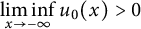 $\liminf \limits _{x\to -\infty } u_0(x)>0$
, then
 $$ \begin{align} \lim\limits_{t\to+\infty}\sup_{x\in \mathbb{R}} |u(t,x;u_0)-U(t,x-ct)|=0. \end{align} $$
By the proof of Step 1 in Theorem 3.7(2), it suffices to show that
 $\lim \limits _{t\to +\infty }\sup _{x\leq -\mu t} |u(t,x;u_0)-U(t,x-ct)|=0$
for some fixed
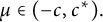 $\mu \in (-c,c^*).$
Due to
 $U(t,-\infty )=p(t)$
and
 $U_\xi (t,\xi )\leq 0$
, it deduces that
 $$ \begin{align*} \sup_{x\leq-\mu t} |p(t)-U(t,x-ct)|=p(t)-\inf_{x\leq-\mu t}U(t,x-ct)=p(t)-U(t,-(\mu+c)t). \end{align*} $$
By the choice of
 $\mu $
, it is easy to see that
 $\mu +c>0$
, then
 $\lim \limits _{t\to +\infty }\sup _{x\leq -\mu t} |p(t)-U(t,x-ct)|=0.$
By the triangular inequality, we shall prove
 $\lim \limits _{t\to +\infty }\sup _{x\leq -\mu t} |u(t,x;u_0)-p(t)|=0.$
Take
 $\delta \in (0,\min \{\mu +c,c^*-c\})$
and some
 $x_0>0$
such that
 $$ \begin{align*} \lim\limits_{t\to+\infty}\sup_{x\leq-\mu t} |u(t,x;u_0)-p(t)|&\leq \lim\limits_{t\to+\infty}\sup_{x\leq-(\mu-\delta) t-x_0} |u(t,x;u_0)-p(t)|\\ &=\lim\limits_{t\to+\infty}\sup_{x\leq-x_0} |u(t,x-(\mu-\delta) t;u_0)-p(t)|. \end{align*} $$
Observe that
 $w(t,x)=u(t,x-(\mu -\delta ) t;u_0)$
satisfies
 $$ \begin{align} \!\!\begin{cases} w_t=w_{xx}-(\mu-\delta)w_x+w[r(t,x-(\mu-\delta+c)t)-w],&t\in(kT^+,(k+1)T],x\in\mathbb{R},\\ w(kT^+,x)=g(w(kT,x)),&x\in\mathbb{R},k\in\mathbb{N},\\ w(0,x)=u_0(x),&x\in\mathbb{R}. \end{cases} \end{align} $$
Let
 $v(t,x)$
be the unique solution of
 $$ \begin{align*} \begin{cases} v_t=v_{xx}-(\mu-\delta)v_x+v[r(t,x)-v],&t\in(kT^+,(k+1)T],x\in\mathbb{R},\\ v(kT^+,x)=g(v(kT,x)),&x\in\mathbb{R},k\in\mathbb{N},\\ v(0,x)=u_0(x),&x\in\mathbb{R}. \end{cases} \end{align*} $$
By the proof of Step 3 in Theorem 3.3,
 $v(t,x)$
has a lower solution, which is similar to (3.2). In addition, it is easy to see that
 $v(t,x)\leq w(t,x)$
for
 $t>0$
and
 $x\in \mathbb {R}$
. Then,
 $w(nT,x)\geq \epsilon _0e^{\gamma _1 T+\frac {\mu -\delta }{2}x}\psi (x)[g'(0)]^{-1},$
where
 $\epsilon _0,\gamma _1,\psi (x)$
are determined by Step 3 in Theorem 3.3. Obviously,
 $\liminf \limits _{x\to -\infty } w(0,x)=\liminf \limits _{x\to -\infty } u_0(x)>0.$
By Lemma 2.1, system (2.1) with
 $u_0=M$
has a unique positive
 $\bar {w}(t;M)$
satisfying
 $\lim \limits _{t\to +\infty }|\bar {w}(t;M)-p(t)|=0.$
Choose
 $M>\sup _{x\in \mathbb {R}} w(0,x)$
, by comparison principle,
 $w(t,x)\leq \bar {w}(t;M)$
for all
 $t>0, x\in \mathbb {R}$
. Thus,
 $$\begin{align*}\lim\limits_{t\to+\infty}\sup_{x\leq-x_0} [w(t,x)-p(t)]\leq \lim\limits_{t\to+\infty}[\bar{w}(t;M)-p(t)]=0.\end{align*}$$
Then, it suffices to prove
 $\lim \limits _{t\to +\infty }\sup _{x\leq -x_0} [p(t)-w(t,x)]\leq 0$
, namely,
 $\forall \epsilon>0$
, there are
 $t_0>0$
and
 $x_0>0$
satisfying
 $\inf _{x\leq -x_0}w(t,x)>p(t)-\epsilon , \forall t\geq t_0.$
For any
 $\epsilon>0$
, there exists
 $\gamma>0$
sufficiently small such that
 $\bar {r}(-\infty )-\gamma>0$
. By Lemma 2.1, equation (2.2) with
 $r(t,-\infty )$
replaced by
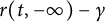 $r(t,-\infty )-\gamma $
has the unique positive solution
 $\beta (t)$
satisfying
 $\beta (t)>p(t)-\frac {\epsilon }{2}$
. For such
 $\gamma $
and
 $w(t,x)$
, we can find
 $y_0<0$
such that
 $r(t,y_0)\geq r(t,-\infty )-\gamma $
for all
 $t>0$
and
 $w(0,x)\geq \frac {1}{2}\liminf \limits _{x\to -\infty } w(0,x)$
for
 $x\leq y_0$
. According to
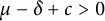 $\mu -\delta +c>0$
and
 $r(\cdot ,x)$
non-increasing in x, we obtain
 $$ \begin{align} r(t,x-(\mu-\delta+c)t)\geq r(t,y_0)\geq r(t,-\infty)-\gamma, \end{align} $$
for any
 $t\geq nT, x-(\mu -\delta +c)nT\leq y_0$
. Define
 $x_n:=y_0+(\mu -\delta +c)nT$
and
 $u_0^n(x):= \epsilon _0e^{\gamma _1 T+\frac {\mu -\delta }{2}x}\psi (x)[g'(0)]^{-1}, x\leq x_n.$
Let
 $w^{n}(t,x;u_0^n)$
be the unique solution of
 $$ \begin{align*} \begin{cases} w^{n}_t=w^{n}_{xx}-(\mu-\delta)w^{n}_x+[r(t,-\infty)-\gamma-w^{n}]w^{n},&t\in(kT^+,(k+1)T],x< x_n,\\ w^{n}(t,x)=0,&t>nT,x=x_n,\\ w^{n}(kT^+,x)=g(w^{n}(kT,x)),&k\geq n, x<x_n,\\ w^{n}(nT,x)=u_0^n(x),&x< x_n. \end{cases} \end{align*} $$
From (2.4) and
 $\mu -\delta \in (-c^*,c^*)$
,
 $\lambda ((-\infty ,x_n])=\lim \limits _{L\to +\infty }\lambda ((x_n-L,x_n]) =\frac {(\mu -\delta )^2}{4}-\frac {(c^*)^2}{4}<0.$
We apply Lemma 2.2 to get that
 $\lim \limits _{m\to +\infty }w^{n}(t+mT,x;u_0^n)=w^{n,*}(t,x), \forall t\in [0,T],x\leq x_n,$
where
 $w^{n,*}(t,x)$
is the unique solution of
 $$ \begin{align*} \begin{cases} w^{n}_t=w^{n,*}_{xx}-(\mu-\delta)w^{n,*}_x+[r(t,-\infty)-\gamma-w^{n,*}]w^{n,*},&t\in(0^+,T],x< x_n,\\ w^{n,*}(t,x)=0,&t\in(0^+,T],x=x_n,\\ w^{n,*}(0^+,x)=g(w^{n,*}(0,x)),& x<x_n,\\ w^{n,*}(0,x)=w^{n,*}(T,x),&x<x_n. \end{cases} \end{align*} $$
Notice that
 $w^{n,*}(t,x)$
is non-increasing in x and increasing in n,
 $w^{n,*}(t,-\infty )=\beta (t)$
. Thus, it follows from
 $x_n\to +\infty $
as
 $n\to \infty $
that there is
 $w^*$
satisfying
 $\lim \limits _{n\to +\infty } w^{n,*}(t,x)=w^*(t,x)$
and
 $w^*(t,x)$
is the solution of
 $$ \begin{align*} \begin{cases} w^*_t=w^*_{xx}-(\mu-\delta)w^*_x+[r(t,-\infty)-\gamma-w^*]w^*,&t\in(0^+,T],x\in\mathbb{R},\\ w^*(0^+,x)=g(w^*(0,x)),& x\in\mathbb{R},\\ w^{*}(0,x)=w^{*}(T,x),&x\in\mathbb{R}. \end{cases} \end{align*} $$
Since
 $w^*(t,y_0)=\lim \limits _{n\to +\infty } w^{n,*}(t,y_0)\geq w^{1,*}(t,y_0)>0$
and
 $\mu -\delta \in (-c^*,c^*),$
we use Louville’s theorem and [Reference Peng and Wei24, Theorem 1.3] to deduce that
 $w^*(t,x)\equiv \beta (t).$
Then, due to (3.11) and
 $w(nT,x)\geq u_0^n(x)$
, from the comparison principle, we get
 $w(t+nT,x)\geq w^n(t+nT,x), \forall t\in (0^+,T],x\leq x_n.$
Consequently,
 $$ \begin{align*} \liminf\limits_{n\to+\infty}\sup_{x\leq y_0} w(nT+t,x)&\geq \liminf\limits_{n\to+\infty}\sup_{x\leq y_0}w^n(t+nT,x)\geq \lim\limits_{n\to+\infty} w^n(t,y_0)=\beta(t)>p(t)-\frac{\epsilon}{2} \end{align*} $$
for all
 $t\in (0^+,T]$
. Taking
 $x_0=-y_0$
, equation (3.9) holds.
Step 3. We shall show equation (3.6).
By equation (3.5), there are
 $T_0>0$
and
 $\rho>0$
satisfying
 $|u(T_0,x)-U(T_0,x-cT_0)|<\rho , \forall x\in \mathbb {R}$
. Taking
 $\xi _0=T_0$
, we know that
 $w^{\pm }$
is a pair of upper–lower solutions of (1.2) for
 $t>T_0$
and
 $x\in \mathbb {R}$
, where
 $w^{\pm }$
is given in Lemma 3.6. It follows from the comparison principle that
 $w^-(t,x)\leq u(t,x)\leq w^+(t,x), \forall t>T_0,x\in \mathbb {R}.$
So,
 $$ \begin{align*} |u(t,x)-U(t,x-ct)|&\leq \rho e^{-\sigma(t-T_0)}[1+M U(t,x-ct)]\\&\leq \rho e^{\sigma T_0}[1+M\max_{[0,T]}p(t)]e^{-\sigma t}, \forall t>T_0,x\in\mathbb{R}. \end{align*} $$
Hence, the proof is complete by letting
 $0<\mu <\sigma $
.
Remark 3.1 As shown in [Reference Fang, Peng and Zhao10], the forced KPP wave of
 $u_t=u_{xx}+ u(r(t,x-ct)-u)$
with initial value
 $u_0(x)$
exists if and only if
 $c<c_F:=2\sqrt {\bar {r}(-\infty )}$
. Assumption (H) implies
 $c^*<c_F$
. By Theorem 3.7, the birth pulse reduces this likelihood that the species moves like a forced KPP wave.
Moreover, we can apply similar arguments to show the propagation dynamics for
 $c\geq c^*$
.
Theorem 3.8 For
 $c\geq c^*$
, if
 $u_0(x)$
is bounded, then
 $$\begin{align*}\lim\limits_{t\to+\infty}\sup_{|x|\leq \mu t} |u(t,x;u_0)-p(t)|=0 \ \text{for any} \ \mu\in(0,c^*).\end{align*}$$
If
 $u_0(x)$
has a compact support, then
 $$\begin{align*}\lim\limits_{t\to+\infty}\sup_{|x|\geq (c^*-\mu) t} u(t,x;u_0)=0 \ \text{for any} \ \mu\in(0,c^*).\end{align*}$$
Proof By the proof of Step 1 in Theorem 3.7(2), for any
 $\epsilon>0$
, there is large enough
 $T_0>0$
satisfying
 $$ \begin{align*} \sup_{x\in[(-c^*+\sigma)t,\xi_0+ct)} |u(t,x;u_0)-p(t)|<\frac{\epsilon}{2}, \forall t\geq T_0, \end{align*} $$
where
 $\xi _0$
is given in Step 1 of Theorem 3.7(2) and
 $\sigma>0$
. Due to
 $c\geq c^*$
and
 $\mu \in (0,c^*)$
, there is large enough
 $T_1>0$
such that
 $\mu t\leq ct+\xi _0$
for
 $t\geq T_1$
. We choose
 $0<\sigma <c^*-\mu $
, then
 $$ \begin{align*} \sup_{|x|\leq \mu t} |u(t,x;u_0)-p(t)|\leq \sup_{x\in[(-c^*+\sigma)t,\xi_0+ct)} |u(t,x;u_0)-p(t)|\kern1.4pt{<}\kern1.4pt\frac{\epsilon}{2}, \forall t\kern1.4pt{\geq}\kern1.4pt \max\{\kern-1pt T_0,T_1\kern-1pt\}. \end{align*} $$
If further
 $u_0(x)$
has a compact support, then it follows from the proof of Theorem 3.7(1) that
 $ u(t+mT,x;u_0)\leq \tilde {w}^{(m)}(t,x)$
and for
 $c\geq c^*$
,
 $$\begin{align*}\tilde{w}^{(m)}(t,x)&=M(e^{-\lambda(-\tilde{L}_t)T}g'(0))^me^{-\lambda(-\tilde{L}_t)t}g'(0)\phi^*(x-ct)\\&\to 0, \forall t\in(0^+,T],x\in \mathbb{R},\text{ as } m\to+\infty .\end{align*}$$
Consequently,
 $$ \begin{align*} 0\leq \lim\limits_{t\to+\infty}\sup_{|x|\geq (c^*-\mu) t} u(t,x;u_0)&\leq\lim\limits_{m\to+\infty}\sup_{|x|\geq (c^*-\mu) s} u(s+mT,x;u_0)\\ &\leq \lim\limits_{m\to+\infty}\sup_{|x|\geq (c^*-\mu) s} \tilde{w}^{(m)}(s,x)=0, \forall s\in(0^+,T]. \end{align*} $$
Hence, our conclusions follow.
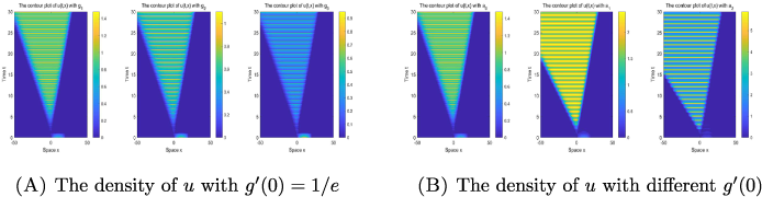
4 Simulations
In this section, we present some simulations to demonstrate our theoretical results, and to illustrate how shifting speed c, impulsive rate
 $g'(0),$
and initial function
 $u_0(x)$
combined affect the long-term behaviors of population dynamics. We truncate infinite domain
 $\mathbb {R}$
to finite domain
 $[-L,L]$
, where L is sufficiently large. Set
 $T=1, L=50,$
and
 $r(t,x)=(2e^{-x}-e^x)(0.8\cos (2\pi t)+1)/(e^{-x}+e^x)$
throughout this section. Obviously,
 $\bar {r}(-\infty )=2$
and
 $\bar {r}(+\infty )=-1$
.
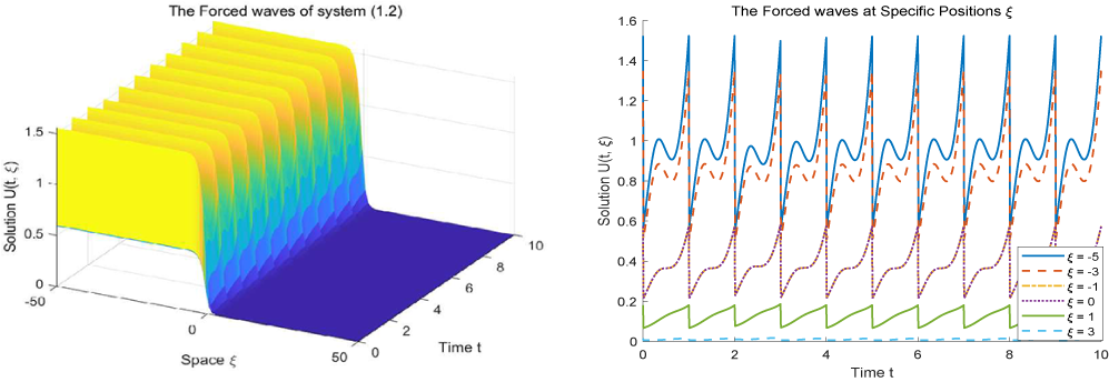
4.1 Forced wave
Let
 $g(u)=au(a>0)$
. In the case where
 $c=-12$
and
 $a=1/e$
. Then,
 $c<c^*=2$
and (H) is satisfied. The simulations of forced waves in a bounded domain
 $[-50,50]$
are shown in Figure 1. It observes that the forced wave
 $U(t,\xi )$
is 1-periodic and non-increasing in
 $\xi $
, which is consistent with the results of Theorem 3.3.
Forced wave for
 $c=-12$
and
 $g'(0)=1/e$
.

4.2 Spatial spread with different shifting speeds c
To simulate the propagation dynamics for different shifting speeds c, we set
 $g(u)=au(a>0)$
with
 $a = 1/e$
, then
 $c^* = 2$
. Meanwhile, we select the initial function
 $u_0(x)$
from the following two options:
 $$\begin{align*}f_1(x) = \begin{cases} 0, & \text{if } -50 \leq x \leq 0 \\ \sin\left(\frac{\pi x}{20}\right), & \text{if } 0 < x < 20 \\ 0, & \text{if } 20 \leq x \leq 50; \end{cases} f_2(x) = \begin{cases} 1, & \text{if } -50 \leq x \leq 0 \\ \cos\left(\frac{\pi x}{40}\right), & \text{if } 0 < x < 20 \\ 0, & \text{if } 20 \leq x \leq 50. \end{cases} \end{align*}$$
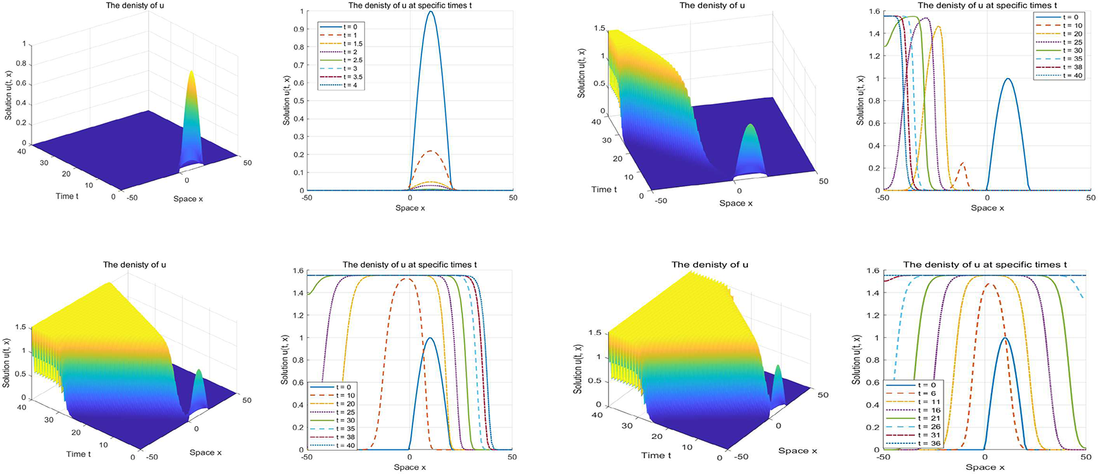
For the initial function
 $u_0(x) = f_1(x)$
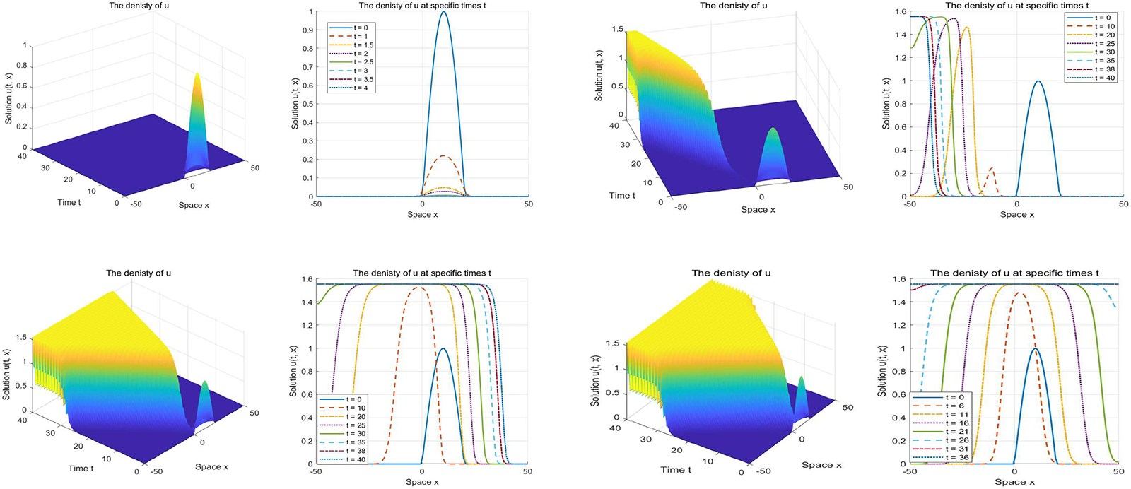
having compact support, the evolution of the solution is shown in Figure 2. It is observed that, for
 $c\leq -c^*$
, the species becomes extinct in any domain as time progresses, which verifies Theorem 3.7(1). If
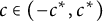 $c \in (-c^*, c^*)$
, then there exists
 $\mu \in (c, c^*)$
such that the density distribution of species u on the domain
 $x> -\mu t$
gradually approaches the shape of the forced wave over time. Furthermore, the direction of the forced wave is determined by the sign of the shifting speed c, consistent with equation (3.5) in Theorem 3.7. Additionally, for
 $c \geq c^*$
, the species will survive and reach a steady state in the core region. Moreover, there exist two transitional regions (buffer zones) where the species density sharply decreases due to shifting environmental factors. Beyond these buffer zones, the species is absent, ultimately leading to extinction, consistent with Theorem 3.8.
The impact of different shifting speeds c on the density of u when
 $u_0=f_1$
(Top left panel
 $c=-5$
; Top right panel
 $c=-1$
; Bottom left panel
 $c=1$
; Bottom right panel
 $c=5$
).
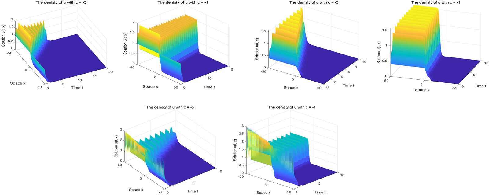
For the initial function
 $u_0(x) = f_2(x)$
, it holds that
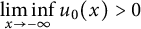 $\liminf \limits _{x \to -\infty } u_0(x)> 0$
and
 $c^* = 2$
. Figure 3 shows that the density distribution of species u across the entire domain gradually approximates the shape of the forced wave as time evolves. Moreover, the direction of the forced wave is determined by the sign of the shifting speed c, consistent with equation (3.9) in Theorem 3.7.
The density of u when
 $u_0=f_2$
(Left panel
 $c=-1$
; Right panel
 $c=1$
).

4.3 Spatial spread with different initial values
$u_0$

To investigate the impact of the initial value
 $u_0(x)$
on propagation dynamics, we still set
 $g(u)=au(a>0)$
with
 $a = 1/e$
, and select
 $u_0(x)$
from functions defined on the domain
 $[-50, 50]$
:
 $f_3(x) =1; f_5(x) = cos(\pi x)+2; f_7(x) =e^{-x^2};$
 $$ \begin{align*} f_4(x) = \begin{cases} 0.4 & \text{if } -50 \leq x \leq 0 \\ 0.4 - 0.04x & \text{if } 0 < x < 10 \\ 0 & \text{if } 10 \leq x \leq 50; \end{cases} \quad f_6(x) = \begin{cases} 0 & \text{if } -50 \leq x \leq 0 \\ 0.06x & \text{if } 0 < x < 10 \\ 0.6 & \text{if } 10 \leq x \leq 50. \end{cases} \end{align*} $$
As shown in Figure 4, Lemma 3.5 still holds for different initial values
 $f_3,f_4,f_5$
, respectively. Then, we provide a guess that the species density u on entire domain approaches the shape of the forced wave over time, as long as
 $c < c^*$
and
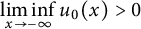 $\liminf \limits _{x \to -\infty } u_0(x)> 0$
. Those give us some direction to weaken the initial value condition in theoretical proofs.
The species density of u under different initial conditions (Top left panel
 $u_0=f_3$
; Top right panel
 $u_0=f_4$
; Bottom panel
 $u_0=f_5$
).

In the case where
 $c\leq -c^*$
or
 $c\geq c^*$
, we select
 $u_0 $
as
 $ f_6$
and
 $f_7$
, respectively, in Figure 5. Note that Theorems 3.7(1) and 3.8 still hold even when the initial value does not have compact support. Thus, we conjecture that Theorems 3.7(1) and 3.8 remain valid under the condition
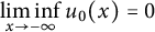 $\liminf \limits _{x \to -\infty } u_0(x) = 0$
.
The species density of u under different initial conditions (Left panel
 $u_0=f_6$
; Right panel
 $u_0=f_7$
).

4.4 Spatial spread with different birth pulses
$g(u)$

To explore the influence of the birth pulse
 $g(u)$
on the propagation dynamics, we set the shifting speed
 $c = 1$
and the initial function
 $u_0(x) = f_1(x)$
. The birth pulse
 $g(u)$
is chosen from one of the following functions:
 $$\begin{align*}g_1(u)=e^{-1}u;g_2(u)=u/(e+u);g_3(u)=e^{-2}ue^{1-u},\end{align*}$$
where
 $g^{\prime }_i(0)=e^{-1}(i=1,2,3)$
satisfies condition (H);
 $g_2$
is the Beverton–Holt function and
 $g_3$
is a Ricker function. Notably,
 $g_1$
and
 $g_2$
are monotone, while
 $g_3$
is non-monotone. As shown in Figure 6(A), the population density varies depending on the form of g. However, when
 $g'(0)$
remains the same, the survival region of species u at any given time remains unchanged, despite variations in the form of g. From the propagation dynamics of u with
 $g = g_3$
, we provide a guess that Theorems 3.7 and 3.8 may still hold even when the birth pulse
 $g(u)$
is non-monotone.
Recalling
 $c^*:=2\sqrt {\bar {r}(-\infty )+\frac {1}{T}\ln g'(0)}$
, we find that the value
 $g'(0)$
will affect the value of
 $c^*$
. In this case, we choose shifting speed
 $c=1$
, the initial function
 $u_0(x)=f_1(x)$
and
 $g(u)=au(a>0)$
with different a. Figure 6(B) shows the population density of u for
 $a=a_i(i=0,1,2)$
, respectively, where
 $a_0=1/e,a_1=1,$
and
 $a_2=e$
. Observe that the density and survival region of species u vary with
 $g'(0)$
; moreover, the survival region expands as
 $g'(0)$
increases, at any given time. Notably, when
 $a = a_1$
, our system (1.2) reduces to the model in [Reference Fang, Peng and Zhao10], indicating that the birth pulse affects the density and survival region of species u. For
 $a = a_2$
, condition (H) is not satisfied; however, the propagation dynamics remain the same. Thus, we conjecture that Theorems 3.7 and 3.8 hold when condition (H) is replaced by
 $e^{\bar {r}(+\infty )}[g'(0)]^{\frac {1}{T}}<1<e^{\bar {r}(-\infty )}[g'(0)]^{\frac {1}{T}}$
.
The species density of
 $u.$

5 Discussion
In this work, we described the propagation dynamics of species giving birth only at a particular time of each period and undergoing a shifting environment with the speed c (the case where the birth pulse is also impacted by the shift of the environment should be considered in future studies). The sign of c indicates if the supportive or adverse environment dominates the invasion process, in our study, we assumed that the environment is supportive at
 $-\infty $
and adverse at
 $+\infty $
. We first defined a forced KPP wave of (1.2), namely,
 $u(t,x)=U(t,x-ct)$
satisfies (1.3)–(1.6). We obtained the existence/nonexistence and uniqueness of forced KPP waves. We have shown that if
 $c<c^*$
, then the forced KPP wave exists and is unique; if
 $c\geq c^*$
, then the forced KPP wave does not exist. We obtained the threshold value
 $c^*$
as the downstream spreading speed of limit system (2.6) and showed that this threshold is determined only by the intrinsic growth rate, the birth pulse, and the period time. It should be emphasized that the maximum spreading speed
 $c^*$
of the forced KPP wave is less than that of in [Reference Fang, Peng and Zhao10], which implies that the birth pulse reduces the possibility that the species eventually moves like a forced KPP wave. In addition, we obtained the propagation behaviors of solutions to (1.2). Our results show that regardless of the direction the environment is moving, as long as the speed of shifting environment is appropriate, the species will eventually propagate like a forced KPP wave, which moves at the same speed as that of the shifting environment. We proved that the forced KPP wave is exponentially stable under some conditions on initial functions. When the shifting speed moves leftward at a large speed, it causes the species extinction in all domains. This occurs because the harsh environment expands rapidly, forcing the species to remain in it for an extended period. When the shifting speed moves rightward at a large speed, the propagation dynamics resemble those of the limiting system in a favorable environment. This is because the species remains in the good environment for a prolonged period.
Finally, our numerical simulations demonstrated that the shifting speed c, the impulsive rate
 $g'(0)$
, and the initial function
 $u_0(x)$
combined will influence the long-term behaviors of population dynamics. Particularly, the survival region of species u at any given time expands as
 $g'(0)$
increases. Our numerical simulations also suggested a conjecture that Theorems 3.7 and 3.8 may remain valid under weaker conditions on the initial values or the birth pulse.
Acknowledgements
We thank the reviewers for their helpful comments and suggestions.
Data availability statement
All data supporting the findings of this study are provided within the article.