1 Introduction
Swimming bacteria with flagella are self-propelled micro-swimmers in nature, and the swimming strategies of such bacteria vary depending on the number and the position of flagella on the cell body. In bacterial flagella-based propulsion, the major driving force, commonly observed by many flagellated bacteria, comes from a rotary motor which is embedded in the cell body and is connected to the flagellar filament via a universal joint called a hook (Berg & Anderson Reference Berg and Anderson1973; Ramia, Tullock & Phan-Thien Reference Ramia, Tullock and Phan-Thien1993; Purcell Reference Purcell1997; McCarter Reference McCarter2001; Berg Reference Berg2003; Sen, Nandy & Ghosh Reference Sen, Nandy and Ghosh2004; Chattopadhyay & Wu Reference Chattopadhyay and Wu2009; Lauga & Powers Reference Lauga and Powers2009; Stocker Reference Stocker2011; Lauga Reference Lauga2016).
Of the flagellated micro-organisms, monotrichous bacteria such as Vibrio alginolyticus have a single left-handed helical flagellum protruding from one end of the major axis of the rod-shaped cell body. The flagellar motor spins either counterclockwise (CCW) or clockwise (CW), and the rotation of the motor is transmitted by a short, straight hook to the flagellar filament, resulting in directed forward or backward swimming (Homma et al. Reference Homma, Oota, Kojima, Kawagishi and Imae1996; Furuno et al. Reference Furuno, Atsumi, Yamada, Kojima, Nishioka, Kawagishi and Homma1997; Magariyama et al. Reference Magariyama, Masuda, Takano, Ohtani and Kudo2001; Chattopadhyay & Wu Reference Chattopadhyay and Wu2009; Xie et al. Reference Xie, Altindal, Chattopadhyay and Wu2010; Son, Guasto & Stocher Reference Son, Guasto and Stocher2013). This marine bacterium changes its swimming direction by exploiting a finely tuned buckling instability caused by the change of the loaded state of the hook. It is known that the hook is much more flexible than the flagellar filament, differing by several orders of magnitude in bending rigidity, and its length is substantially shorter than that of the filament, yielding a length ratio of approximately 50 (Flynn & Ma Reference Flynn and Ma2004; Sen et al. Reference Sen, Nandy and Ghosh2004; Son et al. Reference Son, Guasto and Stocher2013).
The monotrichous bacterium swims backward by turning the motor CW while the hook is under tension. Then the motor reverses suddenly and the bacterium swims forward, which causes the hook to be in a compressed state. A dynamic stiffening of the hook (loaded state) during steady swimming has been observed through direct measurements (Son et al. Reference Son, Guasto and Stocher2013), and the hook becomes more flexible (relaxed state) on the reversal of the motor’s rotational direction. The bending stiffness of the relaxed hook was measured to be 4–6 times smaller than that of the loaded hook. The reason for this stiffness change can be explained by the motor’s torsional load (Block, Blair & Berg Reference Block, Blair and Berg1989, Reference Block, Blair and Berg1991); that is, when the motor reverses, the hook temporarily unwinds, losing the bending stiffness and becoming susceptible to buckling. The buckling of the hook is followed by the flicking of the bacterium, which eventually takes a straightforward run, possibly in a new direction. This ‘run–reverse–flick’ movement pattern is prevalent in motile monotrichous bacteria in the ocean (Stocker Reference Stocker2011).
Many analytical and numerical results have been presented for the dynamics of single-flagellated microorganisms (Taylor Reference Taylor1952; Hancock Reference Hancock1953; Chwang & Wu Reference Chwang and Wu1971; Higdon Reference Higdon1979; Phan-Thien, Tran-Cong & Ramia Reference Phan-Thien, Tran-Cong and Ramia1987; Ramia et al. Reference Ramia, Tullock and Phan-Thien1993; Ishikawa et al. Reference Ishikawa, Sekiya, Imai and Yamaguchi2007; Hsu & Dillon Reference Hsu and Dillon2009; Ishikawa Reference Ishikawa2009; Shum, Gaffney & Smith Reference Shum, Gaffney and Smith2010; Shum & Gaffney Reference Shum and Gaffney2012). In particular, Chwang & Wu (Reference Chwang and Wu1971) used the resistive-force theory to analyse the helical movement of a microorganism with a spherical head, producing a propulsive force by propagating a helical wave along the filament. They investigated optimal conditions for swimming speed and the hydromechanical efficiency depending on the ratio of the head size and the filament length. Higdon (Reference Higdon1979) and Phan-Thien et al. (Reference Phan-Thien, Tran-Cong and Ramia1987) further analysed the optimal swimming motion by using the slender-body theory and the boundary element (BE) method, respectively, with a wide range of parameters for the geometrical properties of the cell body and flagellum. The BE method has also been widely used to investigate the swimming dynamics of a single-flagellated bacterium near a surface or in the vicinity of another organism (Ramia et al. Reference Ramia, Tullock and Phan-Thien1993; Ishikawa et al. Reference Ishikawa, Sekiya, Imai and Yamaguchi2007; Ishikawa Reference Ishikawa2009). All previous models above, however, do not consider the mechanical properties of the filament and hook. Shum et al. (Reference Shum, Gaffney and Smith2010) and Shum & Gaffney (Reference Shum and Gaffney2012) first proposed a model organism that incorporates an elastic hook, while the filament is still rigid, to explore the function and effect of the hook on the motility of single-flagellated bacteria. The Kirchhoff rod theory combined with the BE method is used for their model dynamics. Recently Park et al. (Reference Park, Kim, Ko and Lim2017) investigated the buckling instability of a single rotating flagellum composed of a flexible filament and hook, while the rotating motor is tethered in space. The dynamics of the flagellum is based on the Kirchhoff rod theory (Lim et al. Reference Lim, Ferent, Wang and Peskin2008; Lim & Peskin Reference Lim and Peskin2012), and the hydrodynamic interaction of the flagellum is described by the regularized Stokes formulation (Olson, Lim & Cortez Reference Olson, Lim and Cortez2013). However, the model used in Park et al. (Reference Park, Kim, Ko and Lim2017) does not include a moving cell body.
In this paper, we introduce a comprehensive model for a freely swimming monotrichous bacterium including a cell body and a flexible helical flagellum equipped with a motor connecting a hook to the cell body. Unlike most of the models in previous studies that consider a flagellum rigidly rotating about its axis, the filament and hook in our model are flexible so that they can bend and twist, as in Park et al. (Reference Park, Kim, Ko and Lim2017). We rotate only the motor CW or CCW to generate the twist and thus a helical wave, which is transmitted along the flagellum to its free end, leads to the rotation of the helical filament. Furthermore, the interaction between the cell body and the flagellum is also taken into account. We use Kirchhoff rod theory to model the elastic helical flagellum (Lim et al. Reference Lim, Ferent, Wang and Peskin2008; Park et al. Reference Park, Kim, Ko and Lim2017) and adopt the penalty idea (Kim & Peskin Reference Kim and Peskin2016) to describe the rigid-body dynamics of the cell body. The interaction between fluid and these immersed materials is represented by the regularized Stokes formulation (Olson et al. Reference Olson, Lim and Cortez2013).
We first validate our mathematical model of a monotrichous bacterium by comparing the swimming speed and power efficiency with those of Higdon (Reference Higdon1979), who used the slender-body theory for Stokes flow and an image system for the cell body. We then investigate the dependence of the swimming speed and the rotation rate of the cell body on various physical parameters such as the rotational frequency of the motor, the fluid property and the geometrical shape of the cell body. Finally we find the critical thresholds of the rotational frequency of the motor and the bending modulus of the hook for the buckling instability and explore the dependence of the buckling angle and the change of the swimming direction after buckling on the physical and geometrical parameters of the model.
2 Mathematical model
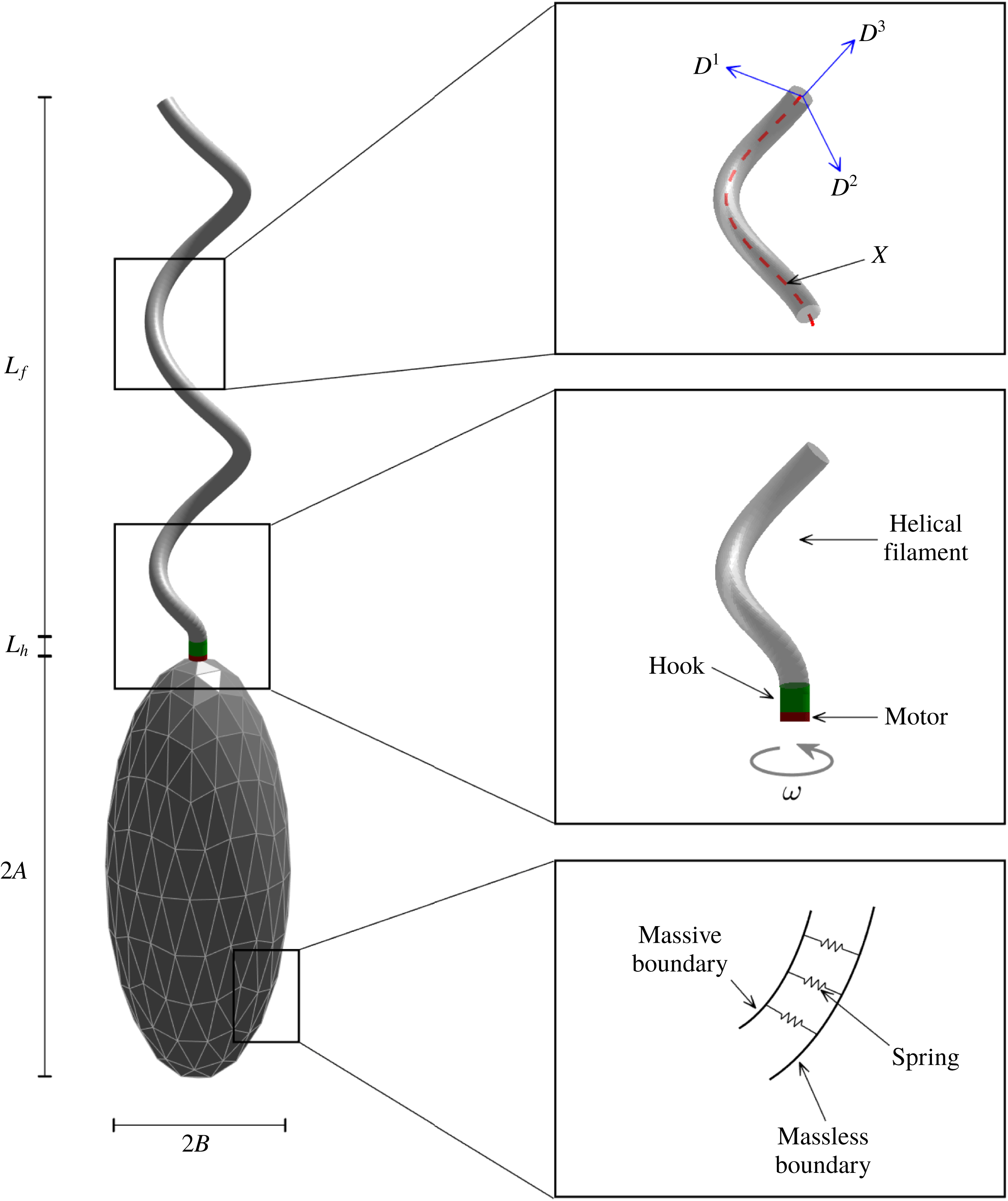
The mathematical model of a single-flagellated bacterium consists of a cell body in the shape of an ellipsoid and a long helical flagellum as a propeller. The flagellum comprises three parts: a rotary motor, a helical filament and a flexible hook that bridges the motor and the filament. See figure 1 for a schematic diagram of our computational model. We describe the elastic flagellar filament and the hook using the Kirchhoff rod model, and use the penalty method to model the cell body as a rigid body. The hydrodynamic interaction between fluid and the bacterium is described by the regularized Stokes formulation (Olson et al. Reference Olson, Lim and Cortez2013).
A schematic view of the computational model for a monotrichous bacterium with a left-handed helical flagellum and an ellipsoidal cell body. The right top panel shows the centreline of a helical rod
 $\boldsymbol{X}$
with an orthonormal triad
 $\{\boldsymbol{D}^{1},\boldsymbol{D}^{2},\boldsymbol{D}^{3}\}$
. The helical flagellar filament is linked to a compliant hook, which is also linked to a rotary motor that is attached at the north pole of the ellipsoidal cell body (right middle). Massive and massless boundaries are linked together by a collection of very stiff springs with zero rest length (right bottom).

2.1 Filament and hook model: Kirchhoff rod theory
In order to model the helical filament and a hook of bacteria, we adopt the Kirchhoff rod theory which uses a space curve
 $\boldsymbol{X}(s,t)$
to represent the centreline of the flagellum and an associated orthonormal triad
 $\boldsymbol{D}^{i}(s,t)$
,
 $i=1,2,3$
, to measure the amount of bending and twisting of the flagellum: see the right-top panel of figure 1. Here,
 $t$
is time and
 $s$
is a Lagrangian coordinate along the rod with
 $0\leqslant s\leqslant L_{h}+L_{f}$
, where
 $L_{h}$
and
 $L_{f}$
are the lengths of the hook and the helical filament, respectively. The initial shape of the helical centreline
 $\boldsymbol{X}(s,0)$
is described as follows (Higdon Reference Higdon1979):
 $$\begin{eqnarray}\boldsymbol{X}(s,0)=(r(s)\cos (\unicode[STIX]{x1D6FC}s),r(s)\sin (\unicode[STIX]{x1D6FC}s),s),\end{eqnarray}$$
where
 $\unicode[STIX]{x1D6FC}$
is the wavenumber and the helical radius
 $r(s)$
is a variable function defined as
 $$\begin{eqnarray}r(s)=\left\{\begin{array}{@{}ll@{}}0\quad & 0\leqslant s\leqslant L_{h},\\ r_{0}(1-\text{e}^{-k_{E}(s-L_{h})^{2}})\quad & L_{h}\leqslant s\leqslant L_{h}+L_{f},\end{array}\right.\end{eqnarray}$$
where
 $k_{E}$
is a constant. The helical radius is 0 for the hook (
 $0\leqslant s\leqslant L_{h}$
) which is a straight rod, and then increases gradually to
 $r_{0}$
for the helical filament (
 $L_{h}\leqslant s\leqslant L_{h}+L_{f}$
).
The vector
 $\boldsymbol{D}^{3}(s,0)$
is initially defined as a unit tangent vector to the helical flagellum (Higdon Reference Higdon1979), and the other two vectors,
 $\boldsymbol{D}^{1}(s,0)$
and
 $\boldsymbol{D}^{2}(s,0)$
, are perpendicular to the tangent vector following the right-hand rule, i.e. normal and binormal vectors to the flagellum. Note that this initial configuration of the centreline and the triad of the helical flagellum are in the equilibrium state in the absence of external forces, and that their deformation from the reference configuration gives rise to the internal energy and force.
Let
 $\boldsymbol{N}(s,t)$
and
 $\boldsymbol{F}(s,t)$
be the moment and the force, respectively, which are transmitted across a section of the rod at the Lagrangian coordinate
 $s$
at time
 $t$
. Let
 $\boldsymbol{f}(s,t)$
and
 $\boldsymbol{n}(s,t)$
be the applied force and the torque densities, respectively. Then the momentum and angular momentum balance equations are described as
 $$\begin{eqnarray}\displaystyle & \displaystyle 0=\,\boldsymbol{f}+\frac{\unicode[STIX]{x2202}\boldsymbol{F}}{\unicode[STIX]{x2202}s}, & \displaystyle\end{eqnarray}$$
 $$\begin{eqnarray}\displaystyle & \displaystyle 0=\boldsymbol{n}+\frac{\unicode[STIX]{x2202}\boldsymbol{N}}{\unicode[STIX]{x2202}s}+\left(\frac{\unicode[STIX]{x2202}\boldsymbol{X}}{\unicode[STIX]{x2202}s}\times \boldsymbol{F}\right), & \displaystyle\end{eqnarray}$$
where all the variables may be expanded in the basis of the orthonormal triad as follows:
 $$\begin{eqnarray}\boldsymbol{F}=\mathop{\sum }_{i=1}^{3}F_{i}\boldsymbol{D}^{i},\quad \boldsymbol{N}=\mathop{\sum }_{i=1}^{3}N_{i}\boldsymbol{D}^{i},\quad \boldsymbol{f}=\mathop{\sum }_{i=1}^{3}f_{i}\boldsymbol{D}^{i},\quad \boldsymbol{n}=\mathop{\sum }_{i=1}^{3}n_{i}\boldsymbol{D}^{i}.\end{eqnarray}$$
The constitutive relations are given by
 $$\begin{eqnarray}N_{i}=a_{i}\left(\frac{\unicode[STIX]{x2202}\boldsymbol{D}^{j}}{\unicode[STIX]{x2202}s}\boldsymbol{\cdot }\boldsymbol{D}^{k}-\unicode[STIX]{x1D6FA}_{i}\right),\end{eqnarray}$$
where
 $(i,j,k)$
is any cyclic permutation of
 $(1,2,3)$
, and
 $$\begin{eqnarray}F_{i}=b_{i}\left(\boldsymbol{D}^{i}\boldsymbol{\cdot }\frac{\unicode[STIX]{x2202}\boldsymbol{X}}{\unicode[STIX]{x2202}s}-\unicode[STIX]{x1D6FF}_{3i}\right),\quad i=1,2,3,\end{eqnarray}$$
where
 $\unicode[STIX]{x1D6FF}_{3i}$
is the Kronecker delta. The coefficients
 $a_{1}$
and
 $a_{2}$
are the bending moduli, and
 $a_{3}$
is the twist modulus of the rod. The coefficients
 $b_{1}$
and
 $b_{2}$
are the shear moduli, and
 $b_{3}$
is the stretching modulus, which controls the degree of inextensibility of the rod. The strain twist vector
 $(\unicode[STIX]{x1D6FA}_{1},\unicode[STIX]{x1D6FA}_{2},\unicode[STIX]{x1D6FA}_{3})$
designates the intrinsic property of the elastic rod in which
 $\unicode[STIX]{x1D705}\equiv \sqrt{\unicode[STIX]{x1D6FA}_{1}^{2}+\unicode[STIX]{x1D6FA}_{2}^{2}}$
is the intrinsic curvature and
 $\unicode[STIX]{x1D6FA}_{3}$
is the intrinsic twist of the rod of which the sign determines the helical handedness of the rod. Negative values of
 $\unicode[STIX]{x1D6FA}_{3}$
correspond to a left-handed helix and positive values of
 $\unicode[STIX]{x1D6FA}_{3}$
correspond to a right-handed helix. We assume that the helical rod is intrinsically left-handed throughout this work. The constitutive relations above can be derived from a variational argument of the elastic energy potential for the unconstrained version of the Kirchhoff rod (Lim et al.
Reference Lim, Ferent, Wang and Peskin2008):
 $$\begin{eqnarray}E=\frac{1}{2}\int _{0}^{L}\left[\mathop{\sum }_{i=1}^{3}a_{i}\left(\frac{\unicode[STIX]{x2202}\boldsymbol{D}^{j}}{\unicode[STIX]{x2202}s}\boldsymbol{\cdot }\boldsymbol{D}^{k}-\unicode[STIX]{x1D6FA}_{i}\right)^{2}+\mathop{\sum }_{i=1}^{3}b_{i}\left(\boldsymbol{D}^{i}\boldsymbol{\cdot }\frac{\unicode[STIX]{x2202}\boldsymbol{X}}{\unicode[STIX]{x2202}s}-\unicode[STIX]{x1D6FF}_{3i}\right)^{2}\right]\text{d}s,\end{eqnarray}$$
where
 $L=L_{h}+L_{f}$
is the total length of the rod, and
 $(i,j,k)$
is any cyclic permutation of
 $(1,2,3)$
. Note that, in the limit
 $b_{3}\rightarrow \infty$
, the rod becomes completely inextensible. In this work, we choose a value of
 $b_{3}$
sufficiently large to make the rod almost inextensible and set
 $a_{1}=a_{2}$
which implies that the rod is isotropic.
2.2 Cell body modelling: penalty method
In order to model a cell body, we use the penalty idea introduced by Kim & Peskin (Reference Kim and Peskin2007, Reference Kim and Peskin2016) to simulate the movement of a massive body interacting with a surrounding fluid. We assume that the cell body is a rigid, hollow ellipsoid which is represented by two Lagrangian descriptions: one is denoted by
 $\boldsymbol{X}_{b}(q,r,t)$
and has no mass, and the other, which we denote by
 $\boldsymbol{Y}_{b}(q,r,t)$
, carries all of the mass and is connected to
 $\boldsymbol{X}_{b}(q,r,t)$
by a system of stiff springs; see the right-bottom panel of figure 1. Here
 $(q,r)$
are parameters for the ellipsoidal surface and
 $t$
is time. The different points on the massive boundary
 $\boldsymbol{Y}_{b}(q,r,t)$
have no direct connection to the fluid and move together as a rigid body in a vacuum, with the only forces and torques applied on the body being the forces generated from the springs that connect the massless description to the massive description of the rigid body.
Since both the massless and massive descriptions are supposed to represent the same body, if a pair of corresponding boundary points moves apart, a restoring force appears in order to make them move close together. The restoring force
 $\boldsymbol{F}_{b}$
acting on the massless boundary is
 $$\begin{eqnarray}\boldsymbol{F}_{b}(q,r,t)=K_{b}(\boldsymbol{Y}_{b}(q,r,t)-\boldsymbol{X}_{b}(q,r,t)),\end{eqnarray}$$
where
 $K_{b}$
is a constant. This defines the force density
 $\boldsymbol{F}_{b}$
which is applied by the massless component
 $\boldsymbol{X}_{b}(q,r,t)$
of the cell body to the fluid so that
 $\boldsymbol{F}_{b}(q,r,t)\,\text{d}q\,\text{d}r$
is the force transmitted to the fluid by the area element
 $\text{d}q\,\text{d}r$
of the cell body. By Newton’s third law, a negative force density
 $-\boldsymbol{F}_{b}(q,r,t)$
acts on the rigid cell body.
In order to describe the rigid-body dynamics, let
 $\boldsymbol{Y}_{cm}(t)$
be the centre of mass of the body, and let
 $\{\boldsymbol{E}_{1}(t),\boldsymbol{E}_{2}(t),\boldsymbol{E}_{3}(t)\}$
be the orthonormal basis for a coordinate system fixed to the body with its origin at the centre of mass. Then the position corresponding to the material point (
 $q,\,r$
) of the body can be written as
 $$\begin{eqnarray}\boldsymbol{Y}_{b}(q,r,t)=\boldsymbol{Y}_{cm}(t)+c_{1}(q,r)\boldsymbol{E}_{1}(t)+c_{2}(q,r)\boldsymbol{E}_{2}(t)+c_{3}(q,r)\boldsymbol{E}_{3}(t).\end{eqnarray}$$
After we introduce two notations – one is a
 $3\times 3$
matrix
 ${\mathcal{E}}(t)$
of which the
 $i$
th column is the
 $3\times 1$
vector
 $\boldsymbol{E}_{i}(t)$
, and the second is the
 $3\times 1$
vector-valued function
 $\boldsymbol{C}(q,r)$
of which the
 $i$
th component is
 $c_{i}(q,r)$
– we can rewrite the position of the cell body as
 $$\begin{eqnarray}\boldsymbol{Y}_{b}(q,r,t)=\boldsymbol{Y}_{cm}(t)+{\mathcal{E}}(t)\boldsymbol{C}(q,r).\end{eqnarray}$$
Since the coordinates are fixed to the body, the coefficients
 $c_{i}(q,r)$
and
 $\boldsymbol{C}(q,r)$
are independent of time.
Now the equations of motion of the rigid body
 $\boldsymbol{Y}_{b}(q,r,t)$
are composed of the translational motion of the centre of mass and the rotational motion of the whole body about the centre of mass. The translational motion can be described as follows:
 $$\begin{eqnarray}\displaystyle & \displaystyle \frac{\text{d}\boldsymbol{Y}_{cm}}{\text{d}t}=\boldsymbol{V}_{cm}(t), & \displaystyle\end{eqnarray}$$
 $$\begin{eqnarray}\displaystyle & \displaystyle M\frac{\text{d}\boldsymbol{V}_{cm}}{\text{d}t}=-\int \boldsymbol{F}_{b}(q,r,t)\,\text{d}q\,\text{d}r, & \displaystyle\end{eqnarray}$$
where
 $\boldsymbol{V}_{cm}(t)$
is the velocity of the centre of mass, and
 $M$
is the total mass of the hollow cell body which can be computed by
 $M=\int m(q,r)\,\text{d}q\,\text{d}r$
, where
 $m(q,r)$
is the mass density of the cell body. Here and in the following, any integral with respect to
 $q,\,r$
is understood to extend over the whole of the immersed body, i.e. the surface of the ellipsoidal cell body.
The rotational motion of the cell body can be summarized as
 $$\begin{eqnarray}\displaystyle & \displaystyle \boldsymbol{T}(t)=\int (\boldsymbol{Y}_{b}(q,r,t)-\boldsymbol{Y}_{cm}(t))\times (-\boldsymbol{F}_{b}(q,r,t))\,\text{d}q\,\text{d}r, & \displaystyle\end{eqnarray}$$
 $$\begin{eqnarray}\displaystyle & \displaystyle \frac{\text{d}\boldsymbol{L}}{\text{d}t}=\boldsymbol{T}(t), & \displaystyle\end{eqnarray}$$
 $$\begin{eqnarray}\displaystyle & \displaystyle \unicode[STIX]{x1D734}(t)={\mathcal{E}}(t)\unicode[STIX]{x1D644}_{0}^{-1}{\mathcal{E}}(t)^{\text{T}}\boldsymbol{L}(t), & \displaystyle\end{eqnarray}$$
 $$\begin{eqnarray}\displaystyle & \displaystyle \frac{\text{d}\boldsymbol{E}_{i}}{\text{d}t}=\unicode[STIX]{x1D734}(t)\times \boldsymbol{E}_{i}(t),\quad i=1,2,3, & \displaystyle\end{eqnarray}$$
where
 $\boldsymbol{T}$
and
 $\boldsymbol{L}$
represent the total torque acting on the cell body and its angular momentum, respectively, and
 $\unicode[STIX]{x1D6FA}(t)$
is the angular velocity of the body. In (2.16), the time-independent matrix
 $\unicode[STIX]{x1D644}_{0}$
, which is called the initial moment of the inertial tensor, can be computed by
 $\unicode[STIX]{x1D644}_{0}=\int m(q,r)(\boldsymbol{C}^{\text{T}}\boldsymbol{C}\unicode[STIX]{x1D644}_{3}-\boldsymbol{C}\boldsymbol{C}^{\text{T}})\,\text{d}q\,\text{d}r$
, where
 $\unicode[STIX]{x1D644}_{3}$
is a
 $3\times 3$
identity matrix. For the detailed derivation for the formula, the readers can refer to Kim & Peskin (Reference Kim and Peskin2016).
Note that, if
 $\boldsymbol{X}_{b}(q,r,t)$
were given, equations (2.9)–(2.17) would be complete and give the rigid-body motion. In order to compute the unknown massless representation
 $\boldsymbol{X}_{b}(q,r,t)$
of the rigid body, we need to take into account the hydrodynamic interaction between
 $\boldsymbol{X}_{b}(q,r,t)$
and the fluid, which will be discussed later in § 2.4.
2.3 Motor linking the hook and the cell body
We equip the bottom end of the hook with a rotary motor which is also attached at the north pole of the ellipsoidal cell body: see the right-middle panel of figure 1. The motor turns either CW or CCW at a prescribed angular velocity
 $\unicode[STIX]{x1D714}$
and generates the twist which is transmitted along the flagellum to its free end and hence leads to the rotation of the whole helical filament.
Since the cell body and the hook are both moving in time and physically share the motor point at the north pole, it is not only necessary to connect the hook to the cell body through the motor point, but we also need to align the direction of the hook with the direction of the cell body at the motor point. To do this, let
 $\boldsymbol{X}(0,t)$
be the bottom end of the hook,
 $\{\boldsymbol{D}^{1}(0,t),\boldsymbol{D}^{2}(0,t),\boldsymbol{D}^{3}(0,t)\}$
be its associated orthonormal triad and
 $\boldsymbol{Y}_{b}^{n}(t)$
be the north pole of cell body at time
 $t$
. We assume that the third basis
 $\boldsymbol{E}_{3}(t)$
of the body is in the same direction as
 $\boldsymbol{Y}_{b}^{n}(t)-\boldsymbol{Y}_{cm}(t)$
. Notice that, if we initially choose the orthonormal basis to satisfy this condition, it continues to hold over time. Then we define the feedback force and moment densities as follows:
 $$\begin{eqnarray}\displaystyle & \displaystyle \boldsymbol{f}_{m}(t)=K_{m}^{1}(\boldsymbol{Y}_{b}^{n}(t)-\boldsymbol{X}(0,t)), & \displaystyle\end{eqnarray}$$
 $$\begin{eqnarray}\displaystyle & \displaystyle \boldsymbol{n}_{m}(t)=K_{m}^{2}(\boldsymbol{E}_{3}(t)\times \boldsymbol{D}^{3}(0,t)), & \displaystyle\end{eqnarray}$$
where
 $K_{m}^{1}$
and
 $K_{m}^{2}$
are sufficiently large constants.
The force density
 $\boldsymbol{f}_{m}(t)$
at the motor point is added to the force density
 $\boldsymbol{f}$
in (2.3) at the bottom end point of the hook
 $\boldsymbol{X}(0,t)$
and expresses that, if the two points
 $\boldsymbol{X}(0,t)$
and
 $\boldsymbol{Y}_{b}^{n}(t)$
move apart, a restoring force comes into play in order to make them move close together. The negative force density
 $-\boldsymbol{f}_{m}(t)$
should also be added to
 $\boldsymbol{F}_{b}(q,r,t)$
at
 $\boldsymbol{Y}_{b}^{n}(t)$
and affects the total force and torque on the cell body. The moment density
 $\boldsymbol{n}_{m}(t)$
at the motor point is added to the moment
 $\boldsymbol{n}$
in (2.4) at
 $\boldsymbol{X}(0,t)$
, which expresses that, if the two vectors
 $\boldsymbol{D}^{3}(0,t)$
and
 $\boldsymbol{E}_{3}(t)$
are not aligned, a restoring moment appears in order to rotate the triad
 $\boldsymbol{D}^{3}(0,t)$
towards
 $\boldsymbol{E}_{3}(t)$
as close as possible. The negative moment
 $-\boldsymbol{n}_{m}(t)$
is also added to the total torque
 $\boldsymbol{T}(t)$
on the cell body.
Now we rotate the motor point at the frequency
 $\unicode[STIX]{x1D714}$
about the tangent vector
 $\boldsymbol{D}^{3}(0,t)$
. This can be done by defining the orthonormal triad at the motor point
 $\boldsymbol{X}(0,t)$
as follows:
 $$\begin{eqnarray}\boldsymbol{D}^{i}(0,t)={\mathcal{R}}(\boldsymbol{D}^{3}(0,t))\boldsymbol{D}_{mot}^{i}(t),\quad i=1,2,\end{eqnarray}$$
where
 ${\mathcal{R}}(\boldsymbol{D}^{3}(0,t))$
represents a rotational matrix to transform the unit vector
 $(0,0,1)$
to the unit vector
 $\boldsymbol{D}^{3}(0,t)=(T_{1}(t),T_{2}(t),T_{3}(t))$
and has the form
 $$\begin{eqnarray}\left(\begin{array}{@{}ccc@{}}T_{3}(t)+T_{2}(t)^{2}/(1+T_{3}(t)) & -T_{1}(t)T_{2}(t)/(1+T_{3}(t)) & T_{1}(t)\\ -T_{1}(t)T_{2}(t)/(1+T_{3}(t)) & T_{3}(t)+T_{1}(t)^{2}/(1+T_{3}(t)) & T_{2}(t)\\ -T_{1}(t) & -T_{2}(t) & T_{3}(t)\end{array}\right).\end{eqnarray}$$
The two orthonormal vectors
 $\boldsymbol{D}_{mot}^{i}(t),\,i=1,2$
, represent the vectors which are rotated at frequency
 $\unicode[STIX]{x1D714}$
from the two standard bases
 $(1,0,0)$
and
 $(0,1,0)$
, respectively, and have the following forms:
 $$\begin{eqnarray}\displaystyle & \displaystyle \boldsymbol{D}_{mot}^{1}(t)=(\cos (2\unicode[STIX]{x03C0}\unicode[STIX]{x1D714}t),\sin (2\unicode[STIX]{x03C0}\unicode[STIX]{x1D714}t),0), & \displaystyle\end{eqnarray}$$
 $$\begin{eqnarray}\displaystyle & \displaystyle \boldsymbol{D}_{mot}^{2}(t)=(-\text{sin}(2\unicode[STIX]{x03C0}\unicode[STIX]{x1D714}t),\cos (2\unicode[STIX]{x03C0}\unicode[STIX]{x1D714}t),0), & \displaystyle\end{eqnarray}$$
where
 $t$
is the time in seconds and
 $\unicode[STIX]{x1D714}$
is the rotation rate in Hz. The sign of
 $\unicode[STIX]{x1D714}$
determines the direction of rotation, i.e.
 $\unicode[STIX]{x1D714}>0$
corresponds to CCW rotation and
 $\unicode[STIX]{x1D714}<0$
corresponds to CW rotation when the rod is viewed towards the motor from the helical filament. Note that we do not prescribe the dynamics (velocity and position) of the flagellum, which was done in the previous studies (Chwang & Wu Reference Chwang and Wu1971; Higdon Reference Higdon1979; Phan-Thien et al.
Reference Phan-Thien, Tran-Cong and Ramia1987; Fujita & Kawai Reference Fujita and Kawai2001). Instead, we rotate the triad only at the motor point, which is more realistic, and the rotation of the motor applies the torque to the hook and then to the helical filament which can rotate together.
2.4 Regularized Stokes formulation
The bacterium is immersed in a viscous fluid which is governed by the incompressible Stokes equations
 $$\begin{eqnarray}\displaystyle & 0=-\unicode[STIX]{x1D735}p+\unicode[STIX]{x1D707}\unicode[STIX]{x0394}\boldsymbol{u}+\boldsymbol{g}, & \displaystyle\end{eqnarray}$$
 $$\begin{eqnarray}\displaystyle & 0=\unicode[STIX]{x1D735}\boldsymbol{\cdot }\boldsymbol{u}, & \displaystyle\end{eqnarray}$$
where
 $\unicode[STIX]{x1D707}$
is the fluid viscosity. The unknown variables
 $\boldsymbol{u}$
,
 $p$
and
 $\boldsymbol{g}$
are the fluid velocity, pressure and the external force per unit volume applied to the fluid, respectively, and they are functions of the fixed Cartesian coordinates
 $\boldsymbol{x}$
and the time
 $t$
. The force density
 $\boldsymbol{g}$
in (2.24) is given as the regularized form
 $$\begin{eqnarray}\displaystyle \boldsymbol{g}(\boldsymbol{x},t) & = & \displaystyle \int _{0}^{L}(-\boldsymbol{f}(s,t))\unicode[STIX]{x1D713}_{\unicode[STIX]{x1D716}}(\boldsymbol{x}-\boldsymbol{X}(s,t))\,\text{d}s+\frac{1}{2}\unicode[STIX]{x1D735}\times \int _{0}^{L}(-\boldsymbol{n}(s,t))\unicode[STIX]{x1D713}_{\unicode[STIX]{x1D716}}(\boldsymbol{x}-\boldsymbol{X}(s,t))\,\text{d}s\nonumber\\ \displaystyle & & \displaystyle +\,\int \boldsymbol{F}_{b}(q,r,t)\unicode[STIX]{x1D713}_{\unicode[STIX]{x1D716}}(\boldsymbol{x}-\boldsymbol{X}_{b}(q,r,t))\,\text{d}q\,\text{d}r,\end{eqnarray}$$
where the first two terms on the right-hand side are the force from the elastic rod (hook and filament), and the last term is the force contributed from the cell body. The radially symmetric blob function
 $\unicode[STIX]{x1D713}_{\unicode[STIX]{x1D716}}$
is defined as
 $$\begin{eqnarray}\unicode[STIX]{x1D713}_{\unicode[STIX]{x1D716}}(\boldsymbol{r})=\frac{15\unicode[STIX]{x1D716}^{4}}{8\unicode[STIX]{x03C0}(|\boldsymbol{r}|^{2}+\unicode[STIX]{x1D716}^{2})^{7/2}},\end{eqnarray}$$
where
 $\unicode[STIX]{x1D716}$
is the regularization parameter and
 $\boldsymbol{r}=\boldsymbol{x}-\boldsymbol{X}$
for a point
 $\boldsymbol{x}$
in the fluid (Cortez Reference Cortez2001; Olson et al.
Reference Olson, Lim and Cortez2013). The blob function
 $\unicode[STIX]{x1D713}_{\unicode[STIX]{x1D716}}$
is a bell-shaped function with infinite support and satisfies
 $\iiint _{\boldsymbol{R}^{3}}\unicode[STIX]{x1D713}_{\unicode[STIX]{x1D716}}(\boldsymbol{r})\,\text{d}\boldsymbol{r}=1$
, spreading most of the force and moment within a ball with the radius
 $\unicode[STIX]{x1D716}$
with its centre at the rod
 $\boldsymbol{X}$
or at the body
 $\boldsymbol{X}_{b}$
. Equation (2.26) describes how we apply the force and torque generated in the immersed body to the fluid, and this implies that the rate at which the immersed body works on the fluid is written in terms of the force and moment applied to the fluid (Lim et al.
Reference Lim, Ferent, Wang and Peskin2008).
Together with (2.3)–(2.7), (2.9)–(2.17) and (2.24)–(2.26), the coupled system of equations closes with the addition of the following equations:
 $$\begin{eqnarray}\displaystyle & \displaystyle \boldsymbol{w}(\boldsymbol{x},t)={\textstyle \frac{1}{2}}\unicode[STIX]{x1D735}\times \boldsymbol{u}(\boldsymbol{x},t), & \displaystyle\end{eqnarray}$$
 $$\begin{eqnarray}\displaystyle & \displaystyle \frac{\unicode[STIX]{x2202}\boldsymbol{X}(s,t)}{\unicode[STIX]{x2202}t}=\boldsymbol{u}(\boldsymbol{X}(s,t),t), & \displaystyle\end{eqnarray}$$
 $$\begin{eqnarray}\displaystyle & \displaystyle \frac{\unicode[STIX]{x2202}\boldsymbol{D}^{i}(s,t)}{\unicode[STIX]{x2202}t}=\boldsymbol{w}(\boldsymbol{X}(s,t),t)\times \boldsymbol{D}^{i}(s,t),\quad i=1,2,3, & \displaystyle\end{eqnarray}$$
 $$\begin{eqnarray}\displaystyle & \displaystyle \frac{\unicode[STIX]{x2202}\boldsymbol{X}_{b}(q,r,t)}{\unicode[STIX]{x2202}t}=\boldsymbol{u}(\boldsymbol{X}_{b}(q,r,t),t). & \displaystyle\end{eqnarray}$$
Equation (2.28) is the relation between the fluid angular velocity
 $\boldsymbol{w}$
and the fluid velocity
 $\boldsymbol{u}$
, both of which are solved using a regularized Stokes formulation. The interaction between the elastic rod and the fluid is described in (2.29) and (2.30) which are the no-slip conditions for the velocity and the angular velocity, respectively. These equations imply that the centreline of the rod translates at the local fluid velocity and that the triad rotates at the local fluid angular velocity. See Olson et al. (Reference Olson, Lim and Cortez2013) and Lee et al. (Reference Lee, Kim, Olson and Lim2014) for a more detailed description of both the mathematical formulation and its numerical scheme. The interaction between the cell body and the fluid is described in (2.31) which also represents the no-slip condition.
Computational and physical parameters.

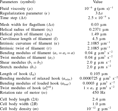
Table 1 shows the computational and physical parameters used in this paper. The fluid viscosity
 $\unicode[STIX]{x1D707}$
is the same as that of water. We compute the intrinsic strain vector
 $(\unicode[STIX]{x1D6FA}_{1},\unicode[STIX]{x1D6FA}_{2},\unicode[STIX]{x1D6FA}_{3})$
from the initial shape of the helical filament given in (2.1) and (2.2). Since the radius of the helical filament increases continuously from 0 to
 $r_{0}$
, the intrinsic strain vector is also a variable function. The intrinsic curvature
 $\unicode[STIX]{x1D705}=\sqrt{\unicode[STIX]{x1D6FA}_{1}^{2}+\unicode[STIX]{x1D6FA}_{2}^{2}}$
and twist
 $\unicode[STIX]{x1D70F}=\unicode[STIX]{x1D6FA}_{3}$
given in table 1 correspond to the values of a helical filament with a constant radius
 $r_{0}$
. Note that we use the exponent
 $k_{E}>2$
in (2.2) and, thus, the majority of our filament model has an approximately constant helical radius
 $r_{0}$
. The cell body is of the shape of a prolate spheroid which has a long axis denoted as body length,
 $2A$
, and two short equal axes denoted as body width,
 $2B$
. Note that the bending modulus of the relaxed hook is approximately 4 times smaller than that of the loaded hook. The relaxed state begins with the reversal of the motor from CW to CCW and lasts for a short period of time. The loss of the stiffness of the hook will be shown to be a crucial factor for the buckling of the hook. Table 1 presents parameter values of the prototype of our bacterium model. In the following sections, however, we vary those physical parameters pertaining to the filament, cell body and the fluid to investigate how these parameters affect the dynamics of swimming bacteria.
3 Results and discussion
3.1 Numerical validation of the model
In this section, we validate the present mathematical model of a single-flagellated bacterium by comparing our simulation results with those of Higdon (Reference Higdon1979), who used slender-body theory for Stokes flow and an image system for the cell body.
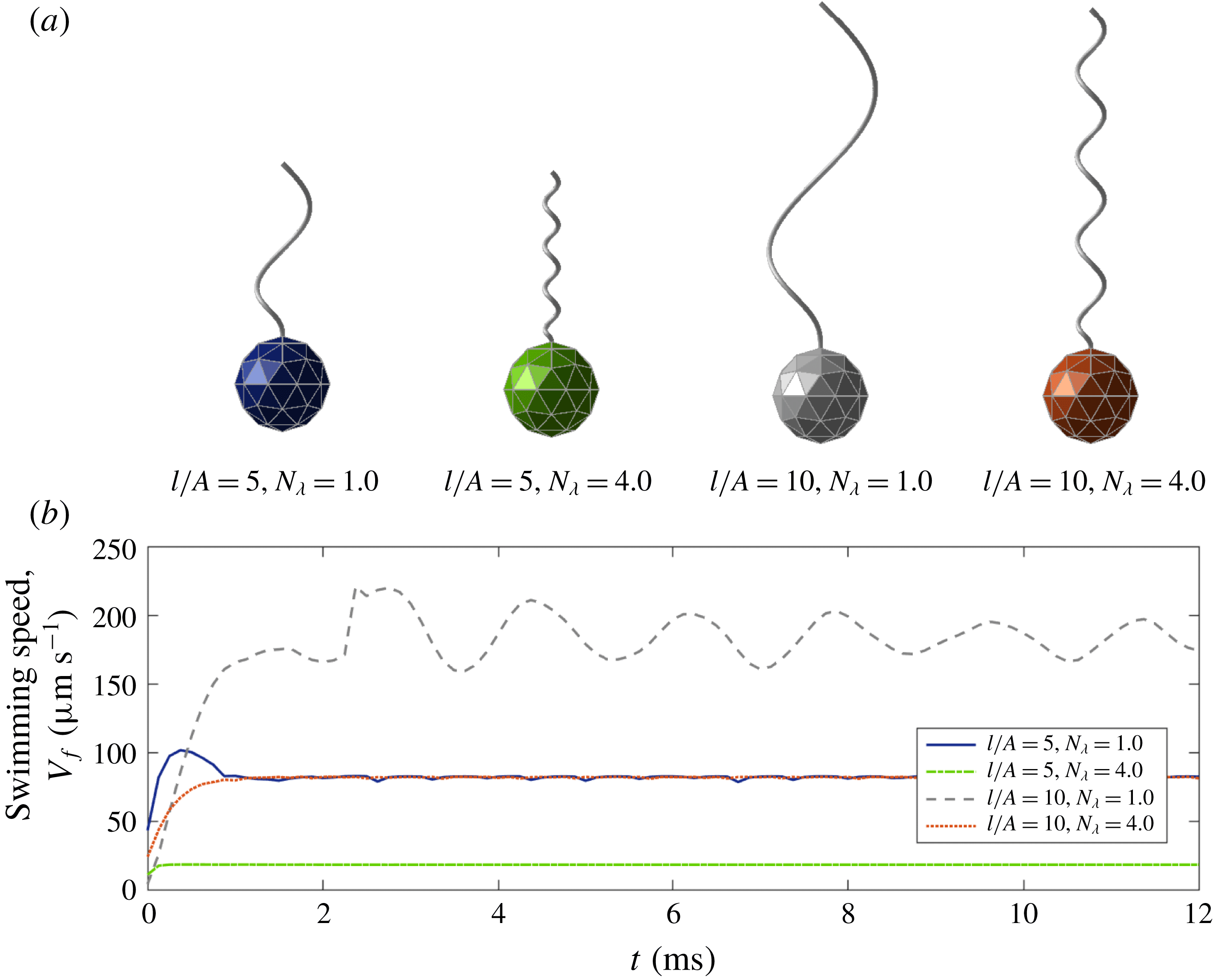
(a) The four different configurations of the model organism depending on
 $l/A$
and
 $N_{\unicode[STIX]{x1D706}}=L_{f}/p_{0}$
, and (b) the corresponding swimming speeds
 $V_{f}(t)$
of the cell body as functions of time. The bacteria eventually reach steady forward swimming motions with small oscillations.

As in Higdon (Reference Higdon1979), we construct a bacterium with a spherical cell body of radius
 $A=0.9~\unicode[STIX]{x03BC}\text{m}$
and a left-handed helical flagellum of two different arc lengths
 $l=4.5~\unicode[STIX]{x03BC}\text{m}$
and
 $9~\unicode[STIX]{x03BC}\text{m}$
. A difference in the helical shape can be generated by changing the helical radius
 $r_{0}$
, helical pitch
 $p_{0}$
and the linear length of the helix
 $L_{f}$
while we fix
 $2\unicode[STIX]{x03C0}r_{0}/p_{0}=1$
and
 $p_{0}\,k_{E}=2\unicode[STIX]{x03C0}$
. Figure 2(a) shows bacteria with four different configurations depending on the ratio of the flagellum length and the sphere radius,
 $l/A$
, and the number of waves,
 $N_{\unicode[STIX]{x1D706}}=L_{f}/p_{0}$
. The motor in the model rotates CCW at the frequency
 $\unicode[STIX]{x1D714}$
when viewed from the flagellum towards the motor, which induces the forward swimming of the micro-organism because the flagellum is intrinsically left-handed and the wave propagates from the motor to the distal end of the flagellum (Lim & Peskin Reference Lim and Peskin2012; Ko et al.
Reference Ko, Lim, Lee, Kim, Berg and Peskin2017). Since the vector
 $\boldsymbol{E}_{3}(t)$
is a unit vector from the centre of mass of the cell body to the north pole, we can compute the directional swimming speed of the cell body as
 $$\begin{eqnarray}V_{f}(t)=-\boldsymbol{V}_{cm}(t)\boldsymbol{\cdot }\boldsymbol{E}_{3}(t).\end{eqnarray}$$
If
 $V_{f}>0$
, the bacterium swims forward, and if it is negative, the bacterium swims backward. Figure 2(b) shows the forward swimming speed
 $V_{f}(t)$
as a function of time for various values of
 $l/A$
and
 $N_{\unicode[STIX]{x1D706}}$
. We can see that the bacteria reach steady forward swimming motions with small oscillations.
Now we define the average swimming speed
 $\overline{V}_{f}$
as the average value of the directional swimming speed
 $V_{f}(t)$
over time after the micro-organism reaches the steady swimming motion with small oscillations. Since there is an oscillatory motion of the cell body,
 $\boldsymbol{E}_{3}(t)$
is not perfectly aligned with the direction of the motion of the cell. Thus,
 $V_{f}(t)$
is not equal to the swimming speed in the direction of average motion, and
 $\overline{V}_{f}$
is not equal to the net displacement of the cell body over the elapsed time. However, since the bacterium swims straight on average,
 $\overline{V}_{f}$
is very close to the forward (
 $z$
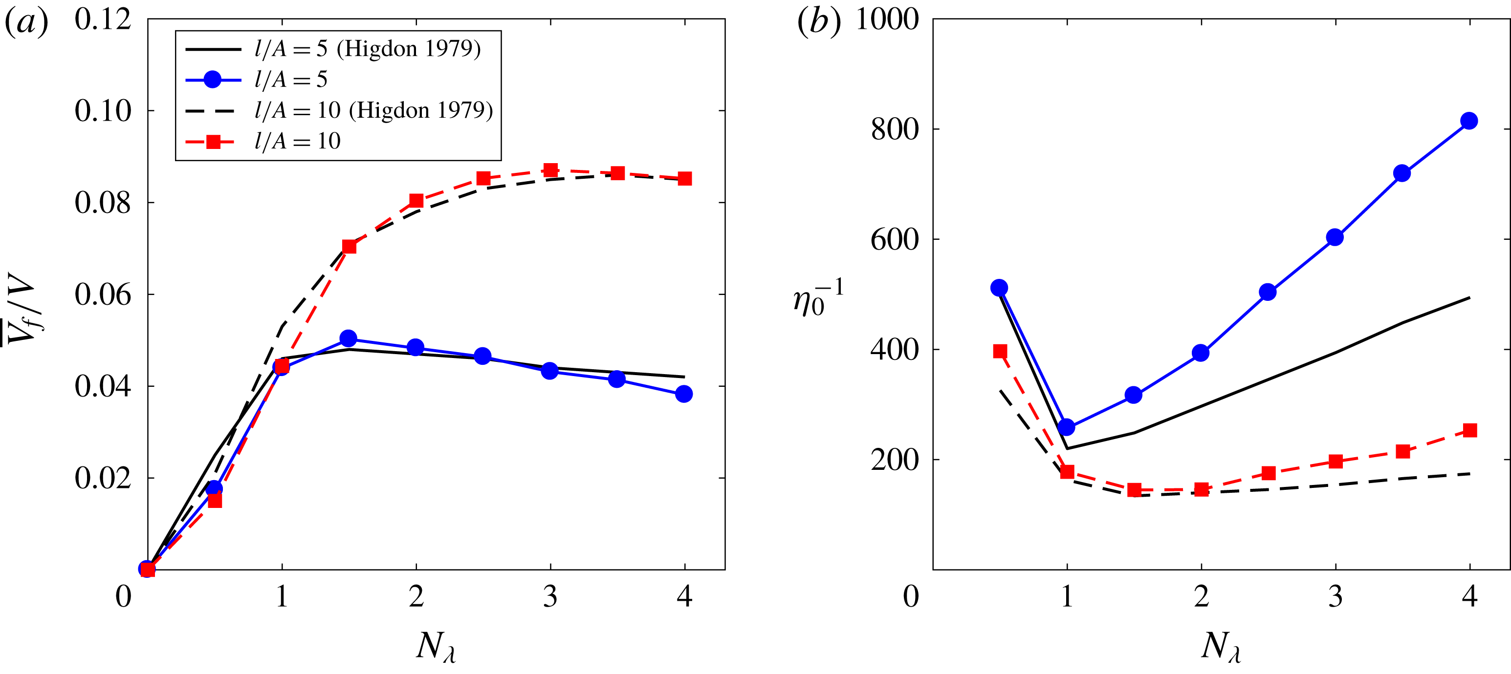
-) directional displacement of the cell body over the elapsed time. Figure 3(a) shows the average swimming speed normalized by the linear wave speed
 $V=\unicode[STIX]{x1D714}\,p_{0}/(2\unicode[STIX]{x03C0})$
of the rotating helical flagellum, i.e.
 $\overline{V}_{f}/V$
for two different ratios
 $l/A$
and various values of
 $N_{\unicode[STIX]{x1D706}}$
. Our numerical results for the average swimming speed are in a good agreement with those in Higdon (Reference Higdon1979) and Phan-Thien et al. (Reference Phan-Thien, Tran-Cong and Ramia1987), which are almost identical.
Normalized average forward swimming speed
 $\overline{V}_{f}/V$
(a) and non-dimensional power consumption
 $\unicode[STIX]{x1D702}_{0}^{-1}$
(b) as functions of the number of waves
 $N_{\unicode[STIX]{x1D706}}$
. The curves compare our numerical results with those in Higdon (Reference Higdon1979) for two different ratios of the flagellum length and the sphere radius
 $l/A=5$
and 10.

The power consumption of the flagellum to move the whole body, which measures how efficient the swimming mechanism is, can be computed by the following formula:
 $$\begin{eqnarray}{\mathcal{P}}(t)=\int _{0}^{L}\boldsymbol{f}(s,t)\boldsymbol{\cdot }\boldsymbol{u}(\boldsymbol{X}(s,t),t)\,\text{d}s.\end{eqnarray}$$
Let
 $\overline{{\mathcal{P}}}$
be the power consumption averaged over time when the micro-organism reaches the steady swimming motion; then we can define the dimensionless power consumption
 $\unicode[STIX]{x1D702}_{0}^{-1}$
by the following formula:
 $$\begin{eqnarray}\unicode[STIX]{x1D702}_{0}^{-1}=\frac{\overline{{\mathcal{P}}}}{6\unicode[STIX]{x03C0}\unicode[STIX]{x1D707}A\overline{V}_{f}^{2}}.\end{eqnarray}$$
Figure 3(b) shows the dimensionless power consumption
 $\unicode[STIX]{x1D702}_{0}^{-1}$
in terms of
 $N_{\unicode[STIX]{x1D706}}$
for two different ratios of the flagellum length and the sphere radius
 $l/A=5$
and 10. The power consumption of our mathematical model is generally larger than the data in Higdon (Reference Higdon1979), which implies that more power is needed for the bacteria to swim forward in our model than the model in Higdon (Reference Higdon1979). The reason for this discrepancy might lie in the difference in the properties of the rotating flagellum: whereas the flagellum model in Higdon (Reference Higdon1979) is perfectly rigid and rotates as a rigid body, our flagellum model is flexible and rotates by the torque which is generated by the spinning motor and transmitted along the flexible flagellum.
Even though the power consumptions of our model are quantitatively different from the data in Higdon (Reference Higdon1979), qualitative agreement is shown in figure 3(b). In particular, a higher value of ratio
 $l/A$
requires a smaller power consumption for the forward swimming, and the power consumptions in both models achieve the optimal values approximately at
 $N_{\unicode[STIX]{x1D706}}=1$
for
 $l/A=5$
and
 $N_{\unicode[STIX]{x1D706}}=1.5$
for
 $l/A=10$
.
3.2 Forward and backward swimming motions
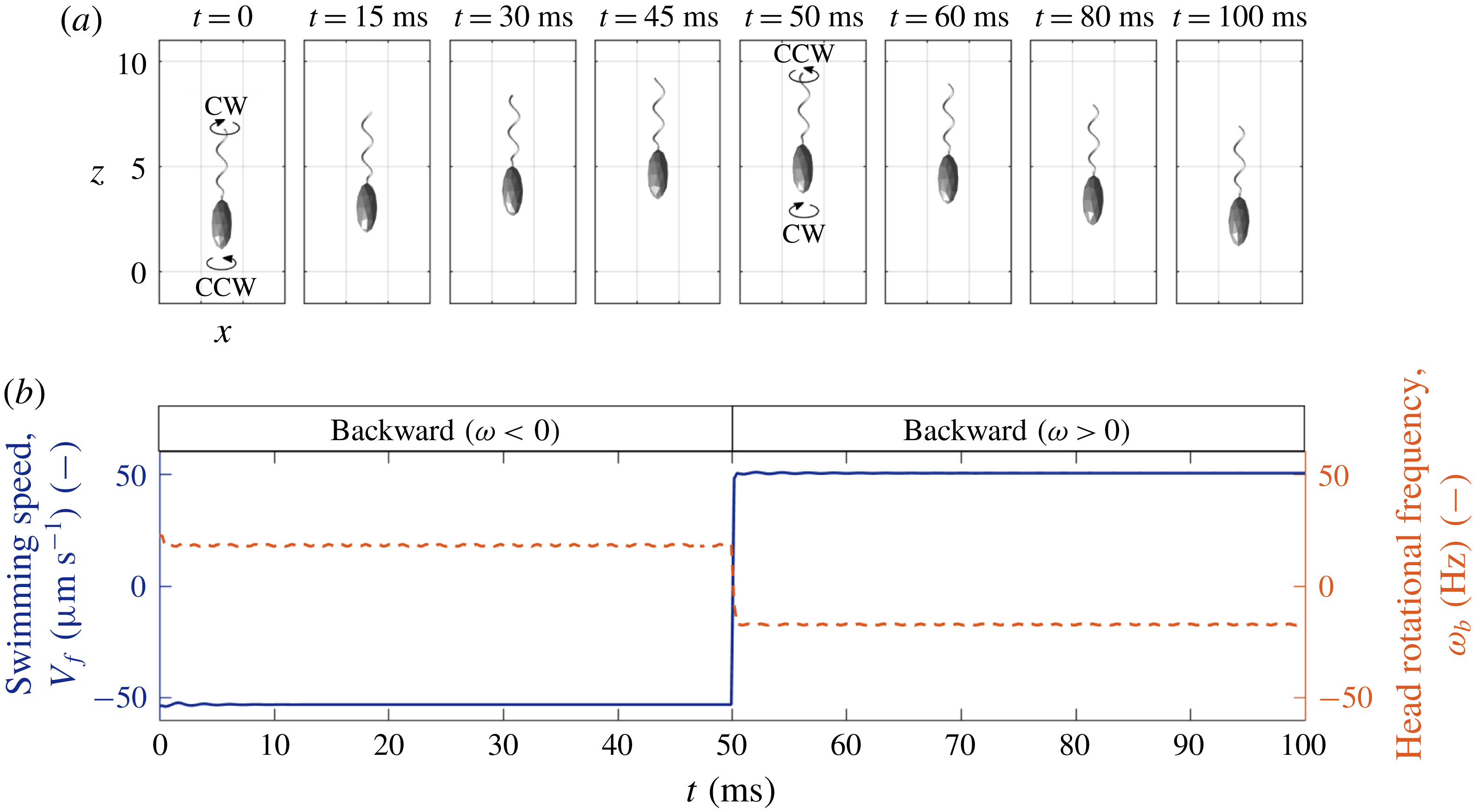
(a) The time evolution of backward and forward swimming motions: when the motor rotates CW (CCW), the cell body counter-rotates and the bacterium swims backward (forward). (b) The directional swimming speed (solid line) and the rotational frequency of the cell body (dashed line). The positive and negative signs of the cell body frequency correspond to CCW and CW rotations, respectively.

V. alginolyticus swims straight backward and forward by rotating the motor CW and CCW, respectively. In order to see the bacterial motion along a straight line, a model bacterium adopts the physical and geometrical parameter values shown in table 1; see also figure 1 for the initial configuration of the model. Note that the single flagellum attached to the cell body is intrinsically left-handed. The motor first rotates CW till
 $t=50~\text{ms}$
and then switches to CCW rotation. Figure 4(a) shows the swimming motion of the bacterium at some selected times (see also supplementary movie 1 available at https://doi.org/10.1017/jfm.2018.799), and figure 4(b) shows the directional swimming speed
 $V_{f}(t)$
(solid line) and the head’s rotational frequency
 $\unicode[STIX]{x1D714}_{b}$
(dashed line) as functions of time. The CW rotation of the motor induces the CW rotation of the left-handed flagellum which pushes the fluid in the forward direction and pulls the cell body in the backward direction, resulting in the straight backward bacterial swimming. The forward swimming driven by the CCW rotation of the motor can be explained in the similar manner. During the backward and forward runs, the cell body counter-rotates naturally to balance the torque.
Throughout this section, we use the bending modulus of the hook as a constant value at all times, i.e.
 $a_{hook}=a_{load}=0.0003~\text{g}~\unicode[STIX]{x03BC}\text{m}^{3}~\text{s}^{-2}$
, which allows the bacterium to reverse the swimming direction quickly as the motor alternates its rotational direction. In reality, however, the bending modulus of the hook gets smaller right after the change of the rotational direction of the motor, i.e.
 $a_{load}>a_{hook}=a_{relax}$
, which might induce a buckling instability of the hook. This case will be discussed separately in the next section.
It is known that V. alginolyticus swims faster in the backward direction than in the forward direction (Magariyama et al.
Reference Magariyama, Masuda, Takano, Ohtani and Kudo2001). Figure 4(b) confirms this experimental observation in which, although the motor rotates at the same magnitude of frequency,
 $\unicode[STIX]{x1D714}=\pm 450~\text{Hz}$
, the swimming speed is
 $-53.07~\unicode[STIX]{x03BC}\text{m}~\text{s}^{-1}$
in the backward swimming and
 $50.22~\unicode[STIX]{x03BC}\text{m}~\text{s}^{-1}$
in the forward swimming. It was also observed experimentally (Chwang & Wu Reference Chwang and Wu1971) that while the motor and hence the flagellum rotate in the same direction, the cell body rotates in the opposite direction with an approximate relation
 $\unicode[STIX]{x1D714}=-22\unicode[STIX]{x1D714}_{b}$
where
 $\unicode[STIX]{x1D714}_{b}$
is the rotational frequency of the cell body (Chattopadhyay & Wu Reference Chattopadhyay and Wu2009; Lauga & Powers Reference Lauga and Powers2009; Son et al.
Reference Son, Guasto and Stocher2013). Figure 4(b) also shows that the cell body rotates at
 $\unicode[STIX]{x1D714}_{b}=18.02~\text{Hz}$
during the backward run with
 $\unicode[STIX]{x1D714}=-450~\text{Hz}$
and it rotates at
 $\unicode[STIX]{x1D714}_{b}=-17.36~\text{Hz}$
during the forward run with
 $\unicode[STIX]{x1D714}=450~\text{Hz}$
. In both cases, the ratio
 $\unicode[STIX]{x1D714}/\unicode[STIX]{x1D714}_{b}$
is approximately
 $-25$
.
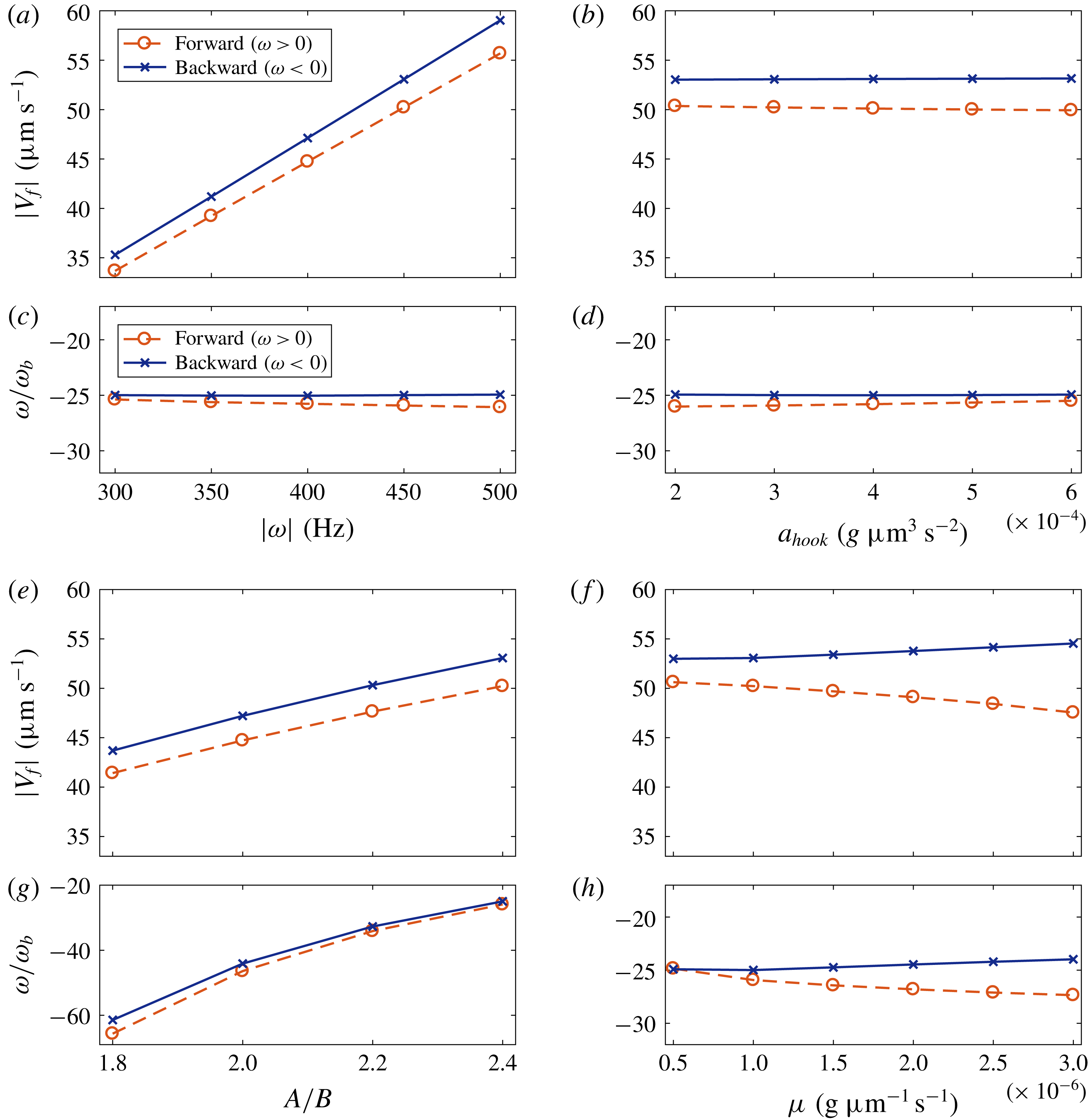
The swimming speed,
 $|V_{f}|$
(a,b,e,f), and the ratio of the rotational frequencies of the motor and the cell body,
 $\unicode[STIX]{x1D714}/\unicode[STIX]{x1D714}_{b}$
(c,d,g,h) in terms of four different parameters: rotational frequency of the motor
 $\unicode[STIX]{x1D714}$
(a,c), bending modulus of the hook
 $a_{hook}$
(b,d), cell body ratio
 $A/B$
(e,g) and fluid viscosity
 $\unicode[STIX]{x1D707}$
(f,h). The lines with ‘○’ and ‘
 $\times$
’ indicate the forward and backward swimming modes, respectively.

We investigate the dependence of the swimming speed and the rotation rate of the cell body on various physical parameters. Each pair of panels in figure 5 shows the absolute value of the swimming speed,
 $|V_{f}|$
(a,b,e,f), and the ratio of the rotational frequencies of the motor and the cell body,
 $\unicode[STIX]{x1D714}/\unicode[STIX]{x1D714}_{b}$
(c,d,g,h) in terms of four different parameters: rotational frequency of the motor
 $\unicode[STIX]{x1D714}$
(a,c), bending modulus of the hook
 $a_{hook}$
(b,d), cell body ratio
 $A/B$
(e,g) and fluid viscosity
 $\unicode[STIX]{x1D707}$
(f,h). When one of the parameters varies, all the other parameters are held fixed at the values given in table 1. The lines with ‘○’ and ‘
 $\times$
’ indicate the forward and backward swimming modes, respectively, and thus CCW and CW rotations of the flagellum, respectively.
Figure 5(a,c) shows that the swimming speed and the rotational frequency of the cell body increase linearly with the angular frequency of the motor and that the ratios of the rotational frequencies of the motor and the cell body stay approximately at a constant value,
 $-25.0$
. The bending modulus of the hook
 $a_{hook}$
has almost no influence on the swimming speed and the cell body rotation within the range of
 $a_{hook}$
given in figure 5(b,d). Note that, if
 $a_{hook}$
is smaller than some critical value and the bacterium swims forward, the hook goes through a buckling instability; see the next section.
Figure 5(e,g) shows that the swimming speed and the rotational speed of the cell body increase as the cell body ratio
 $A/B$
increases. In these simulations, we change the minor axis
 $B$
only while the major axis
 $A$
of the ellipsoidal body is fixed as a constant. As the ratio
 $A/B$
increases and thus
 $B$
decreases, the cell body becomes more slender and experiences a lower drag force from the fluid, which enables the cell body to translate and turn faster.
As the fluid viscosity
 $\unicode[STIX]{x1D707}$
increases, the linear and angular swimming speeds of the cell body increase slightly in the backward swimming mode, but they decrease to a relatively large extent in the forward swimming mode: see figure 5(f,h). This supports that the backward swimming speed is always larger than the forward swimming speed in the natural marine fluid even with the same magnitude of the motor frequency; see also the upper panel of each pair.
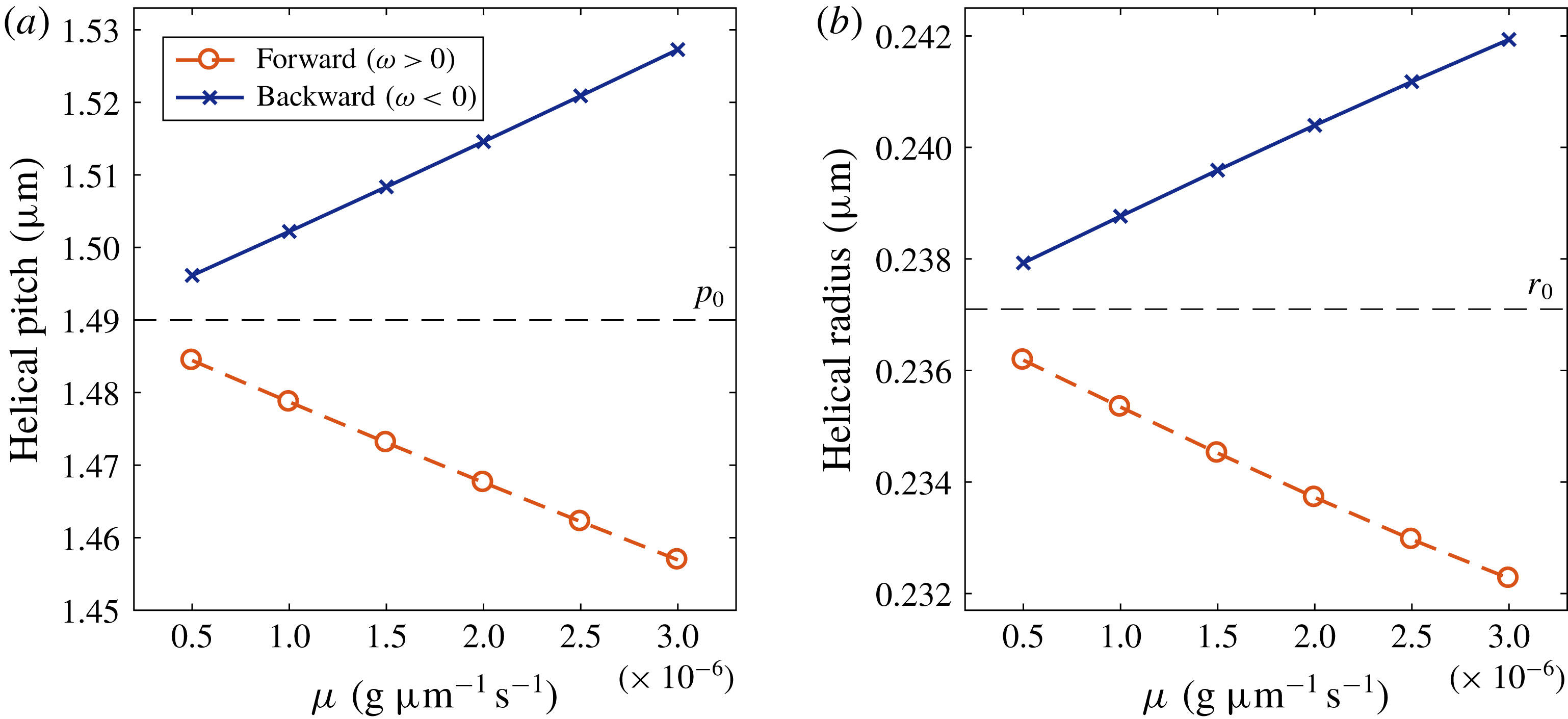
The measured values of the helical pitch (a) and the helical radius (b) of the flagellum in comparison with those of the initial flagellum in the equilibrium state (dashed lines). The bacterium swims forward and backward with
 $\unicode[STIX]{x1D714}=\pm 450~\text{Hz}$
in a fluid with various viscosities.

The difference in the swimming speeds depending on the swimming direction and the fluid viscosity is due to the change of the geometrical properties of the flexible flagellum. Figure 6 depicts the measured values of the helical pitch (a) and helical radius (b) of the flagellum when it swims forward (‘○’) and backward (‘
 $\times$
’) in a fluid with various viscosities in comparison with those of the initial flagellum in the equilibrium state (dashed lines). We can see that the helical pitch and radius become smaller in the forward swimming mode than those of equilibrated flagellum due to the compression while they become larger in the backward swimming mode due to the tension. These differences get larger as the fluid viscosity increases. Ko et al. (Reference Ko, Lim, Lee, Kim, Berg and Peskin2017) demonstrated that the mean fluid flux generated by a rotating helical filament, which implies a swimming speed, depends proportionally on the helical pitch and radius. These proportional relations of the swimming speed with the helical radius and the helical pitch (only when the pitch is large enough) have also been observed in experiments (Rodenborn et al.
Reference Rodenborn, Chen, Swinney, Liu and Zhang2013; Thawani & Tirumkudulu Reference Thawani and Tirumkudulu2017). Thus, as the fluid viscosity increases, the swimming speed gets larger in the backward direction and smaller in the forward direction. Since a faster swimming body experiences a larger drag force from the fluid, the angular swimming speed
 $\unicode[STIX]{x1D714}_{b}$
is inversely proportional to the linear swimming speed: see figure 5(h).
3.3 Buckling instability and reorientation
A monotrichous bacterium V. alginolyticus has a single left-handed helical filament with its bottom end being linked to a short flexible hook (Kawagishi et al. Reference Kawagishi, Imagawa, Imae, McCarter and Homma1996; Kudo et al. Reference Kudo, Imai, Nishitoba, Sugiyama and Magariyama2005). It swims forward and backward by rotating the motor which is embedded in the cell body (Homma et al. Reference Homma, Oota, Kojima, Kawagishi and Imae1996; Goto et al. Reference Goto, Nakata, Baba, Nishimura and Magariyama2005). Since there is no chiral transformation of the helical flagellum during locomotion, it can swim back and forth in a straight line unless the flagellum bends and flicks the cell body. Thus, buckling of the hook plays a significant role in reorientation of swimming direction and the chemotaxis of single-flagellated bacteria.
The hook alternates two states during swimming, loaded and relaxed states, and the two states are distinguished by two different bending rigidities of the hook such that the loaded hook is less flexible than the relaxed hook, i.e.
 $a_{load}>a_{relax}$
. The bacterium swims backward by turning the motor CW while the hook is in the loaded state. Then it suddenly changes the rotational direction of the motor to CCW, which causes the bacterium to swim forward and the hook to be in the relaxed state. The compression of the hook due to the forward swimming and the more flexible hook in the relaxed state may trigger the buckling instability of the flagellum followed by the flick of the bacterium. After a short period of the flick for reorientation of the organism, the hook is again in the loaded state to be straight, and the organism runs steadily forward in a new direction (Son et al.
Reference Son, Guasto and Stocher2013). This swimming pattern of the run–reverse–flick movement is typical in the marine motile bacteria.
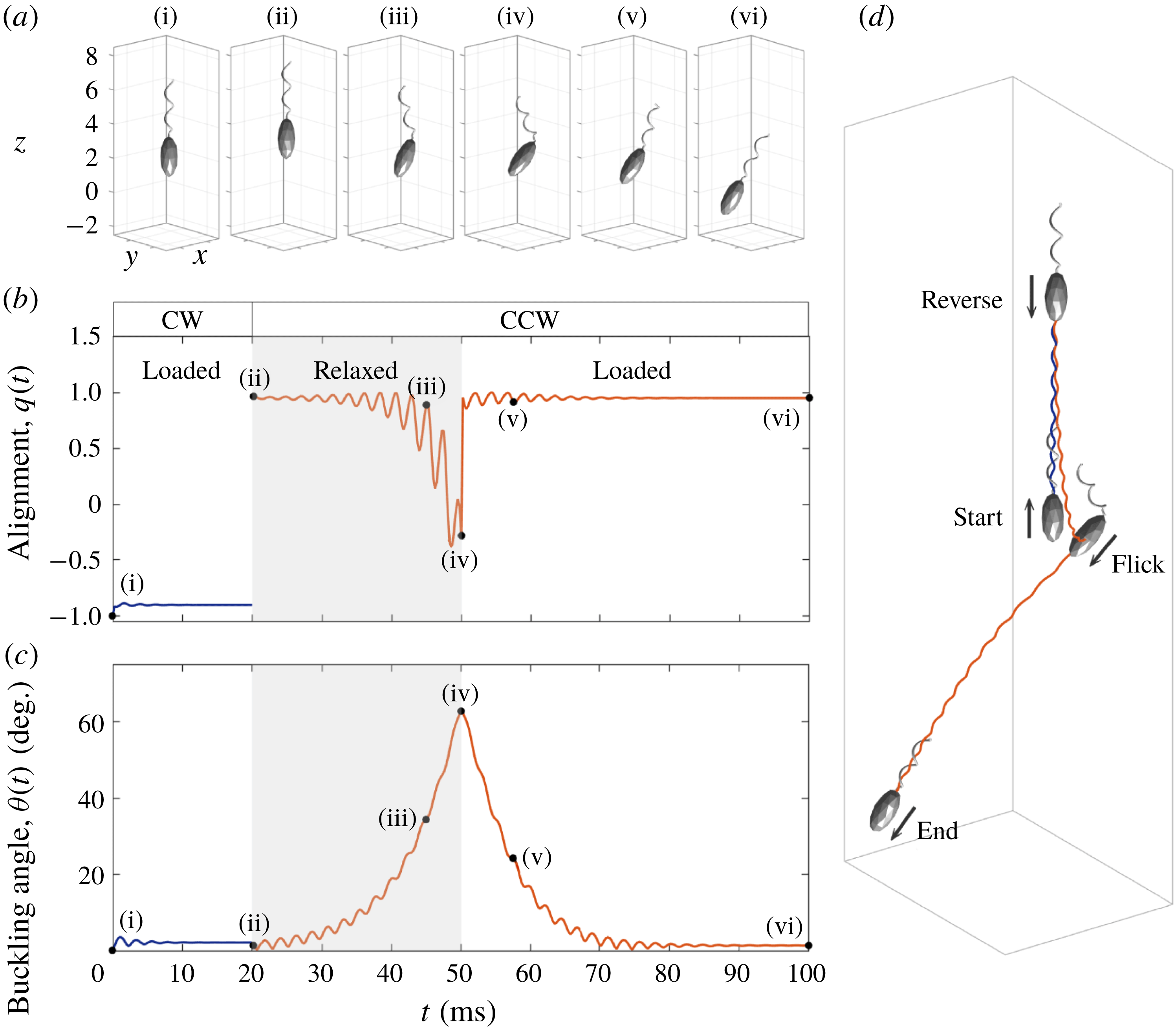
Snapshots at some chosen times (a), the trajectory (d) of the dynamical motion of V. alginolyticus and the time evolutions of the alignment
 $q(t)$
(b) and the buckling angle
 $\unicode[STIX]{x1D703}(t)$
(c). The trajectory of the organism follows the order of start–reverse–flick–end. The motor frequency changes from
 $\unicode[STIX]{x1D714}=-450~\text{Hz}$
to 450 Hz at
 $t=20~\text{ms}$
. The bending modulus of the hook is given as
 $a_{relax}=0.0000725~\text{g}~\unicode[STIX]{x03BC}\text{m}^{3}~\text{s}^{-2}$
in the relaxed state from
 $t=20$
to
 $t=50~\text{ms}$
and
 $a_{load}=0.0003~\text{g}~\unicode[STIX]{x03BC}\text{m}^{3}~\text{s}^{-2}$
in the loaded state.

In order to investigate the buckling instability of the flagellum, we choose the relaxed and loaded bending moduli of the hook as
 $a_{relax}=0.0000725~\text{g}~\unicode[STIX]{x03BC}\text{m}^{3}~\text{s}^{-2}$
and
 $a_{load}=0.0003~\text{g}~\unicode[STIX]{x03BC}\text{m}^{3}~\text{s}^{-2}$
, respectively, which are two or three orders of magnitude lower than that of the flagellar filament as reported in Son et al. (Reference Son, Guasto and Stocher2013). Figure 7 shows the dynamical motion of the computational model for V. alginolyticus (see also supplementary movie 2) and the resulting variations that occur in the organism as it experiences buckling instability. The flagellar motor initially turns CW and the hook is under tension and thus the organism swims backward steadily. At
 $t=20~\text{ms}$
the motor reverses to CCW and the hook is under the relaxed state from
 $t=20$
to
 $t=50~\text{ms}$
. During this time period, there occurs a buckling instability of the hook and the flicking of the cell body. At
 $t=50~\text{ms}$
, the hook becomes loaded again, and the helical filament begins to be aligned with the cell body. When the cell body and the filament are aligned completely, the bacterium swims forward steadily in a new direction. Figure 7(a) shows snapshots taken at six selected times during locomotion of the bacterium which are drawn in the actual size. Figure 7(d) illustrates its trajectory in three-dimensional space following the order of start–reverse–flick–end, in which the size of the bacterium is scaled down for a better visualization.
To investigate more quantitatively the buckling dynamics of the bacterium, we define the following two quantities: the alignment,
 $q(t)$
, between the swimming direction and the cell body orientation which is defined as
 $q(t)=-(\boldsymbol{V}_{cm}(t)\boldsymbol{\cdot }\boldsymbol{E}_{3}(t))/|\boldsymbol{V}_{cm}(t)|$
, and the buckling angle,
 $\unicode[STIX]{x1D703}(t)$
, which is defined by an angle between the cell body axis and the helical axis. We compute the helical axis as a vector from the motor point to the average value of the coordinates of the flagellum. Figure 7(b,c) shows the alignment
 $q(t)$
and the buckling angle
 $\unicode[STIX]{x1D703}(t)$
as functions of time. The alignment
 $q(t)$
is around
 $-1$
(backward swimming) initially and changes into about
 $+1$
(forward swimming) at
 $t=20~\text{ms}$
. Then the flick begins approximately at
 $t=25~\text{ms}$
and lasts up to
 $t=50~\text{ms}$
, which is characterized by the deviation of
 $q(t)$
from
 $\pm 1$
. Then the alignment
 $q(t)$
reaches again
 $+1$
after
 $t=50~\text{ms}$
, which indicates that the swimming direction and the cell body orientation are aligned again. The buckling angle
 $\unicode[STIX]{x1D703}(t)$
is around 0 initially, which implies that the cell body axis and the helical axis are well aligned, and increases up to
 $63^{\circ }$
during the relaxed state of the hook from 20 to 50 ms. Then it begins to decrease after the return of the hook to the loaded state at
 $t=50~\text{ms}$
and eventually gets close to 0 at approximately
 $t=80~\text{ms}$
. This swimming pattern of our mathematical model of V. alginolyticus is in a good agreement with the experimental observation reported in Son et al. (Reference Son, Guasto and Stocher2013).
During backward swimming, the thrust from the flagellum and the drag on the cell body occur in opposite directions and repel away from one another, and thus the hook is under tension. In contrast, during forward swimming, the thrust and drag attract one another and thus the hook is under compression. The compression of the hook triggers the buckling of the hook followed by the flicks of the bacterium, which results in reorientation of the cells. It is known that the hook of V. alginolyticus is a straight, hollow, slender rod with a length of approximately 100 nm and the bending modulus of the hook is 2–3 orders of magnitude smaller than that of the helical filament (Takano et al. Reference Takano, Yoshida, Kudo, Nishitoba and Magariyama2003; Son et al. Reference Son, Guasto and Stocher2013). Thus, the hook can be easily bent when it is compressed. Euler beam theory (Timoshenko Reference Timoshenko1961; Son et al. Reference Son, Guasto and Stocher2013) predicts that a slender rod under axial and torsional loadings buckles when
 $$\begin{eqnarray}F_{h}/F_{cr}+(T_{h}/T_{cr})^{2}>1,\end{eqnarray}$$
where
 $F_{h}$
and
 $T_{h}$
are the typical axial force and torque acting on the rod, respectively,
 $F_{cr}=\unicode[STIX]{x03C0}^{2}\,a_{hook}/L_{h}^{2}$
is the critical load and
 $T_{cr}=2\unicode[STIX]{x03C0}\,a_{hook}/L_{h}$
is the critical torque for buckling of the rod.
In our mathematical model, the axial load
 $F_{h}$
and the torque
 $T_{h}$
acting on the hook can be computed by the following formula:
 $$\begin{eqnarray}F_{h}(t)=-\boldsymbol{f}(0,t)\boldsymbol{\cdot }\boldsymbol{D}^{3}(0,t)\unicode[STIX]{x0394}s;\quad T_{h}(t)=-\boldsymbol{n}(0,t)\boldsymbol{\cdot }\boldsymbol{D}^{3}(0,t)\unicode[STIX]{x0394}s,\end{eqnarray}$$
where
 $\boldsymbol{f}(0,t)$
,
 $\boldsymbol{n}(0,t)$
and
 $\boldsymbol{D}^{3}(0,t)$
are force density, moment density and the unit tangential vector, respectively, at the end point of the hook. Note that the negative sign makes the compression (tension) positive (negative).
The axial load
 $F_{h}$
(a,b) and torque
 $T_{h}$
(c,d) as functions of time when the bacterium swims in the forward direction at two different rotation rates of the motor,
 $\unicode[STIX]{x1D714}=300~\text{Hz}$
(a,c,e) and 450 Hz (b,d,f). The bending modulus of the hook is given as
 $a_{hook}=0.0001~\text{g}~\unicode[STIX]{x03BC}\text{m}^{3}~\text{s}^{-2}$
(solid lines),
 $0.000175~\text{g}~\unicode[STIX]{x03BC}\text{m}^{3}~\text{s}^{-2}$
(dashed lines) and
 $0.00025~\text{g}~\unicode[STIX]{x03BC}\text{m}^{3}~\text{s}^{-2}$
(dotted lines). The load
 $F_{h}$
and torque
 $T_{h}$
approach almost constant values except for the case with
 $a_{hook}=0.0001~\text{g}~\unicode[STIX]{x03BC}\text{m}^{3}~\text{s}^{-2}$
and
 $\unicode[STIX]{x1D714}=450~\text{Hz}$
, in which case the hook buckles. Panel (e) classifies the region into the stable (‘○’) and unstable (‘
 $\times$
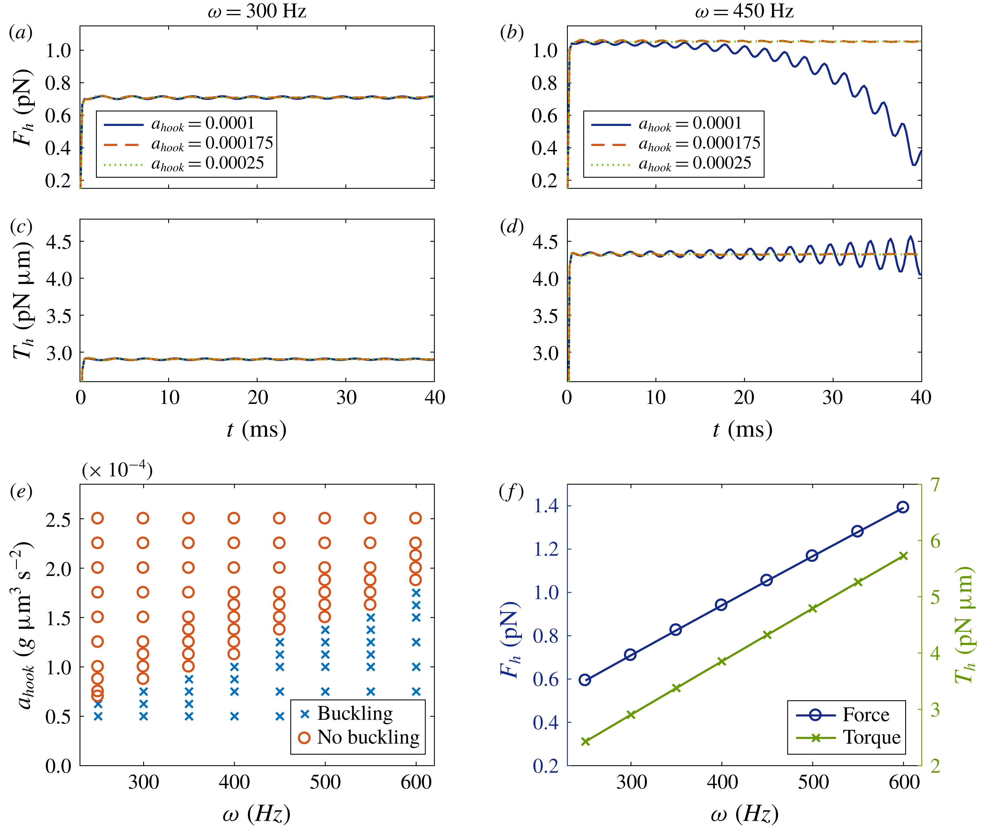
’) hooks as the bending modulus of the hook and the motor frequency are varied. The mean values of the limiting constant values of the load
 $F_{h}$
(‘○’) and the torque
 $T_{h}$
(‘
 $\times$
’) are displayed in terms of the rotational frequency of the motor (f).

Figure 8(a–d) illustrates the load
 $F_{h}$
(upper) and the torque
 $T_{h}$
(middle) as functions of time when the bacterium swims in the forward direction at two different rotation rates of the motor,
 $\unicode[STIX]{x1D714}=300~\text{Hz}$
(a,c) and 450 Hz (b,d). For each rotation rate, we display time evolutions of the load and torque for three different values of the bending modulus of the hook:
 $a_{hook}=0.0001~\text{g}~\unicode[STIX]{x03BC}\text{m}^{3}~\text{s}^{-2}$
(solid lines),
 $0.000175~\text{g}~\unicode[STIX]{x03BC}\text{m}^{3}~\text{s}^{-2}$
(dashed lines) and
 $0.00025~\text{g}~\unicode[STIX]{x03BC}\text{m}^{3}~\text{s}^{-2}$
(dotted lines). Here, all the other parameters are held fixed at the values given in table 1. We can see that, when the bending modulus of the hook
 $a_{hook}$
is larger than some critical values which depend on the rotational frequency of the motor, the load
 $F_{h}$
and the torque
 $T_{h}$
on the hook approach almost the same constant values independent of
 $a_{hook}$
. However, when the motor turns faster or the bending modulus of the hook is smaller than the critical value, there occurs a buckling instability which is indicated by the deviation of the solid line from the other lines as shown in figure 8(b,d).
Collectively, figure 8(e) shows the separation of the stable (‘○’) and unstable (‘
 $\times$
’) regions of the hook as the bending modulus of the hook and motor frequency are varied. It appears that there exists a critical value of the bending modulus of the hook which increases linearly with the motor frequency. While the bending modulus of the hook is fixed, as the rotational frequency of the motor
 $\unicode[STIX]{x1D714}$
increases up to the critical threshold, the load
 $F_{h}$
and torque
 $T_{h}$
increase together in the forward swimming mode. These increments finally drive the hook into the region of the buckling instability.
While the motor frequency is fixed, each bending modulus above the critical value allows no buckling and induces limiting constant values of the force and torque acting on the hook. Figure 8(f) displays the mean of the limiting constant values of the load
 $F_{h}$
(‘○’) and the torque
 $T_{h}$
(‘
 $\times$
’), when there is no buckling instability. In a low Reynolds number flow, the load
 $F_{h}$
and torque
 $T_{h}$
on the hook are linearly proportional to the swimming speed of the cell body (see the supplementary article of Son et al.
Reference Son, Guasto and Stocher2013). Since the swimming speed increases linearly with the rotational frequency of the motor as shown in figure 5(a), the limiting constant values of the load
 $F_{h}$
and torque
 $T_{h}$
are linearly proportional to the rotational frequency of the motor, as confirmed by our simulations.
The occurrence of buckling of the hook can be predicted by Euler beam theory (3.4). For example, since our model sets
 $a_{hook}=0.0000725~\text{g}~\unicode[STIX]{x03BC}\text{m}^{3}~\text{s}^{-2}$
and
 $L_{h}=0.105~\unicode[STIX]{x03BC}\text{m}$
, the critical thresholds are given as
 $F_{cr}=64.9~\text{pN}$
and
 $T_{cr}=4.34~\text{pN}~\unicode[STIX]{x03BC}\text{m}$
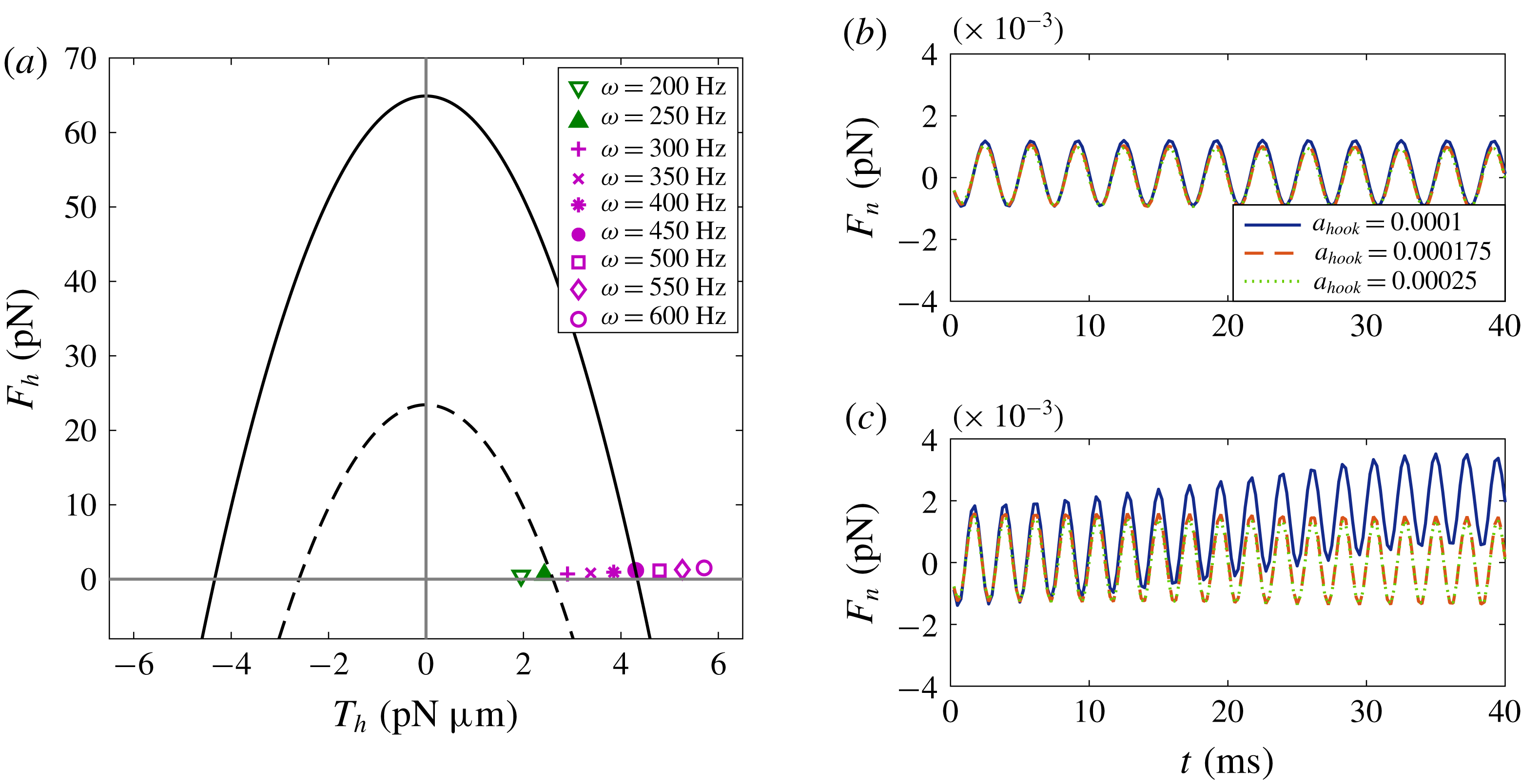
. With these particular values, figure 9(a) draws the buckling instability diagram of the hook with the solid parabola corresponding to
 $F_{h}/F_{cr}+(T_{h}/T_{cr})^{2}=1$
. The markers indicate data points of axial forces and torques corresponding to nine different rotation rates of the motor from our simulations. According to the diagram, the critical frequency of the motor that separates stable from unstable hooks is expected to be approximately
 $\unicode[STIX]{x1D714}=450~\text{Hz}$
. However, this theoretical prediction for the buckling instability does not match with our numerical results shown in figure 8(e), in which the hook is buckled even when
 $\unicode[STIX]{x1D714}=300~\text{Hz}$
.
(a) Stable (no buckling) and unstable (buckling) regions separated by
 $F_{h}/F_{cr}+(T_{h}/T_{cr})^{2}=1$
(solid arc) and
 $F_{h}/F_{cr}+(T_{h}/T_{cr})^{2}=0.36$
(dashed arc) with the markers representing forces and torques in the cases of nine different motor frequencies. The critical loads for the solid curve are determined by
 $a_{hook}=0.0000725~\text{g}~\unicode[STIX]{x03BC}\text{m}^{3}~\text{s}^{-2}$
and
 $L_{h}=0.105~\unicode[STIX]{x03BC}\text{m}$
. (b,c) One of the normal components of force,
 $F_{n}$
, as a function of time for two different frequencies,
 $\unicode[STIX]{x1D714}=300~\text{Hz}$
(b) and
 $450~\text{Hz}$
(c), and three different bending moduli of the hook:
 $a_{hook}=0.0001~\text{g}~\unicode[STIX]{x03BC}\text{m}^{3}~\text{s}^{-2}$
(solid lines),
 $0.000175~\text{g}~\unicode[STIX]{x03BC}\text{m}^{3}~\text{s}^{-2}$
(dashed lines) and
 $0.00025~\text{g}~\unicode[STIX]{x03BC}\text{m}^{3}~\text{s}^{-2}$
(dotted lines).

A possible reason for this discrepancy is that the beam theory uses the typical axial force and torque acting on the rod only in the direction along the rod (tangential direction), without taking into account the normal direction. When the organism moves forward by the rotation of the hook and flagellum, however, the force and torque in the direction perpendicular to the hook might be so large that they affect the condition for the buckling instability. Figure 9(b,c) illustrates one of the normal components of the load, denoted by
 $F_{n}$
, as a function of time when the motor frequency is given as
 $\unicode[STIX]{x1D714}=300~\text{Hz}$
(b) and
 $450~\text{Hz}$
(c), and the bending modulus of the hook is given as
 $a_{hook}=0.0001~\text{g}~\unicode[STIX]{x03BC}\text{m}^{3}~\text{s}^{-2}$
(solid lines),
 $0.000175~\text{g}~\unicode[STIX]{x03BC}\text{m}^{3}~\text{s}^{-2}$
(dashed lines) and
 $0.00025~\text{g}~\unicode[STIX]{x03BC}\text{m}^{3}~\text{s}^{-2}$
(dotted lines). Only when
 $\unicode[STIX]{x1D714}=450~\text{Hz}$
and
 $a_{hook}=0.0001~\text{g}~\unicode[STIX]{x03BC}\text{m}^{3}~\text{s}^{-2}$
, does buckling of the hook occur: see the deviation of the solid line in (c) panel. Even though the normal forces are sinusoidal and have a mean of almost 0, their amplitudes are as large as the corresponding tangential loads shown in figure 8(a,b) and hence might impact on the buckling instability. Using the data shown in figure 8(e,f), we can derive a new prediction that the hook buckles when
 $$\begin{eqnarray}F_{h}/F_{cr}+(T_{h}/T_{cr})^{2}\gtrapprox 0.36,\end{eqnarray}$$
which is represented as the dashed parabola in figure 9(a).
The buckling angle, which might determine the new swimming direction of the bacterium after flicks, can be dependent on the physical properties of the hook, flagellum and cell body. In order to first investigate the dependence of the buckling angle and the swimming direction on the properties of the hook, we vary the following physical parameters of the hook: the relaxed bending modulus
 $a_{relax}$
, the loaded bending modulus
 $a_{load}$
and the twist modulus
 $a_{3}^{hook}$
. The other parameter values are kept the same as in table 1. The motor turns CW at
 $\unicode[STIX]{x1D714}=-450~\text{Hz}$
until
 $t=20~\text{ms}$
and rotates CCW at
 $\unicode[STIX]{x1D714}=450~\text{Hz}$
when
 $t>20~\text{ms}$
. The hook is in the loaded state at all times except for the time interval (20 ms, 50 ms), when it is in the relaxed state.
We measure the swimming direction of the organism using the deviation angle
 $\unicode[STIX]{x1D703}_{z}(t)$
of the cell body axis from the positive
 $z$
-direction which is computed as
 $\unicode[STIX]{x1D703}_{z}(t)=\cos ^{-1}(\boldsymbol{E}_{3}(t)\boldsymbol{\cdot }(\boldsymbol{e}_{3}))$
, where
 $\boldsymbol{e}_{3}$
is the standard unit vector in the positive
 $z$
-direction. Since the vector from the centre to the north pole of the cell body is initially aligned with
 $\boldsymbol{e}_{3}$
, the forward and backward runs both give rise to
 $\unicode[STIX]{x1D703}_{z}=0^{\circ }$
, if there is no change of swimming direction. After buckling of the hook and flicking of the cell body are complete, since the cell body axis and the helical axis are well aligned in the loaded state, the organism reorients and swims forward steadily with a new value of
 $\unicode[STIX]{x1D703}_{z}$
.
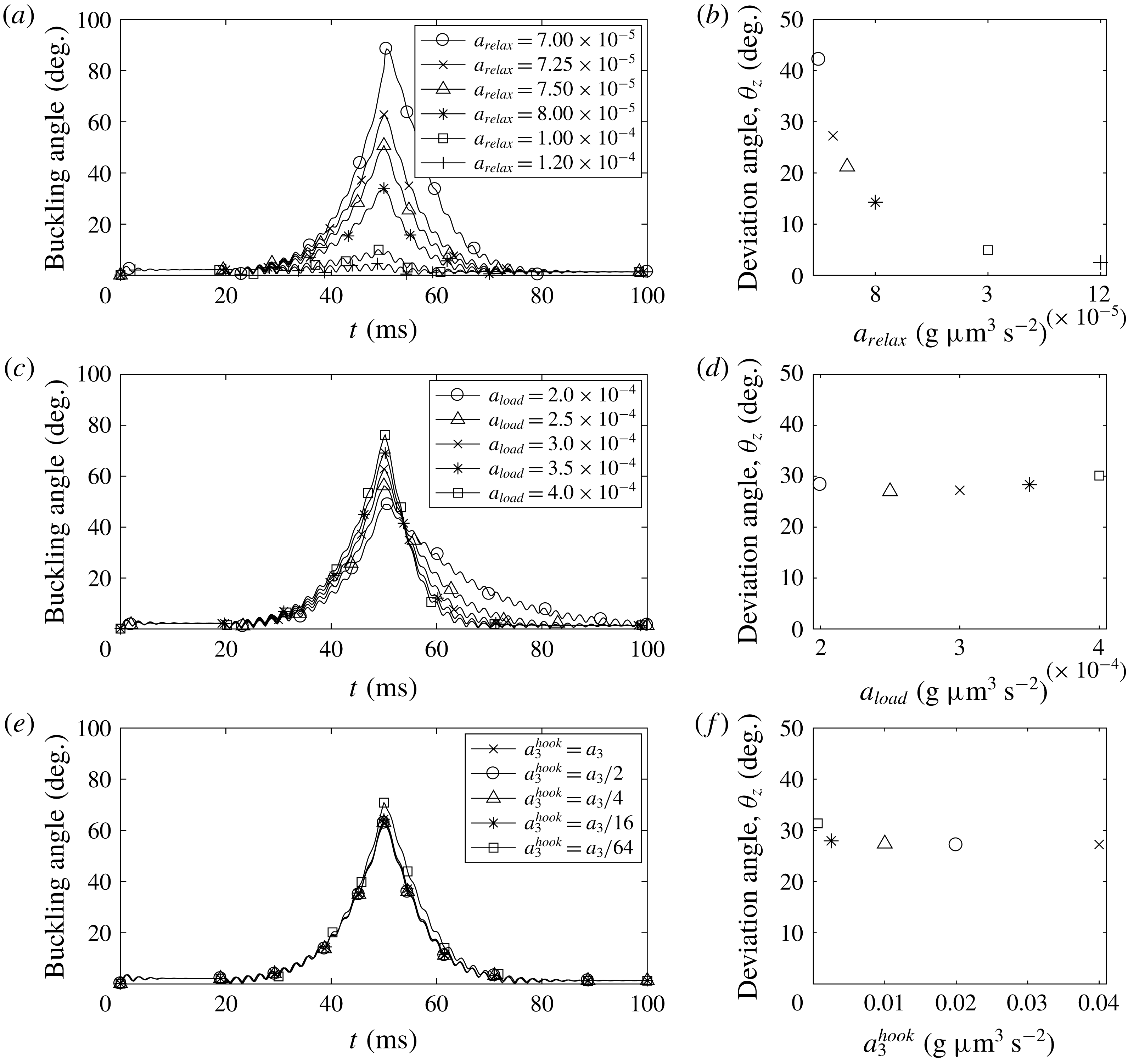
Buckling angle (a,c,e) and steady deviation angle (b,d,f) with various relaxed and loaded bending moduli and twist moduli of the hook. Relaxed bending modulus of the hook varies from
 $0.00007$
to
 $0.00012~\text{g}~\unicode[STIX]{x03BC}\text{m}^{3}~\text{s}^{-2}$
in (a,b), the loaded bending modulus of the hook is changed from
 $0.0002$
to
 $0.0004~\text{g}~\unicode[STIX]{x03BC}\text{m}^{3}~\text{s}^{-2}$
in (c,d), and the twist modulus of the hook is changed to be 1–64 times smaller than that of the helical filament in (e,f). The motor turns CW at
 $\unicode[STIX]{x1D714}=-450~\text{Hz}$
until
 $t=20~\text{ms}$
and rotates CCW at
 $\unicode[STIX]{x1D714}=450~\text{Hz}$
when
 $t>20~\text{ms}$
. The hook is in the loaded state at all times except for
 $20~\text{ms}<t<50~\text{ms}$
, when it is in the relaxed state.

Figure 10(a) shows the time evolution of buckling angles for various bending moduli of the relaxed hook ranging from
 $a_{relax}=0.00007$
to
 $0.00012\;\text{g}~\unicode[STIX]{x03BC}\text{m}^{3}~\text{s}^{-2}$
, while
 $a_{load}=0.0003~\text{g}~\unicode[STIX]{x03BC}\text{m}^{3}~\text{s}^{-2}$
and
 $a_{3}^{hook}=a_{3}$
are fixed. We can see that the maximum buckling angle depends inversely on the bending modulus of the relaxed hook, which is comparable to the results in Park et al. (Reference Park, Kim, Ko and Lim2017). When
 $a_{relax}$
is larger than
 $0.0001~\text{g}~\unicode[STIX]{x03BC}\text{m}^{3}~\text{s}^{-2}$
, the buckling angle is so small that the hook is considered to be stable and no buckling occurs. The deviation angle
 $\unicode[STIX]{x1D703}_{z}$
is closely related to the buckling angle as shown in figure 10(b) in which we draw the constant value of the deviation angle obtained when the organism swims steadily in one direction after the buckling of the hook and the flicking of the cell body are complete. It is shown that the steady deviation angle
 $\unicode[STIX]{x1D703}_{z}$
is also inversely proportional to the bending modulus of the relaxed hook. In particular, when
 $a_{relax}=0.00007~\text{g}~\unicode[STIX]{x03BC}\text{m}^{3}~\text{s}^{-2}$
, the maximum buckling angle is almost 90
 $^{\circ }$
and the steady deviation angle is approximately
 $42^{\circ }$
.
Figure 10(c,d) depicts the time evolution of buckling angles (c) and the steady deviation angles (d) for various bending moduli of the loaded hook ranging from
 $a_{load}=0.0002$
to
 $0.0004~\text{g}~\unicode[STIX]{x03BC}\text{m}^{3}~\text{s}^{-2}$
, while
 $a_{relax}=0.0000725~\text{g}~\unicode[STIX]{x03BC}\text{m}^{3}~\text{s}^{-2}$
and
 $a_{3}^{hook}=a_{3}$
are fixed. Since the buckling threshold depends only on the relaxed bending modulus
 $a_{relax}$
, the buckling instability occurs independently of the loaded bending modulus
 $a_{load}$
(Son et al.
Reference Son, Guasto and Stocher2013; Park et al.
Reference Park, Kim, Ko and Lim2017). However, the loaded bending modulus can change the maximum buckling angle and vary the time elapsed for the restoration of the buckling angle. In spite of these differences in the detailed behaviour of the buckling angle, the steady deviation angles
 $\unicode[STIX]{x1D703}_{z}$
, and thus the swimming directions differ only slightly as the bending modulus of the loaded hook is varied: see figure 10(d).
We also investigate the effect of the twist modulus of the hook
 $a_{3}^{hook}$
while the bending moduli of the hook in the two different states are fixed as
 $a_{relax}=0.0000725~\text{g}~\unicode[STIX]{x03BC}\text{m}^{3}~\text{s}^{-2}$
and
 $a_{load}=0.0003~\text{g}~\unicode[STIX]{x03BC}\text{m}^{3}~\text{s}^{-2}$
. It is shown in figure 10(e) that the buckling angle is almost independent of the twist modulus of the hook. This result follows well the criterion for the buckling instability in (3.4) which does not depend on the twist modulus of the hook. Since the pattern of the buckling angles is similar, the new swimming directions are also similar, as shown in figure 10(f).
g
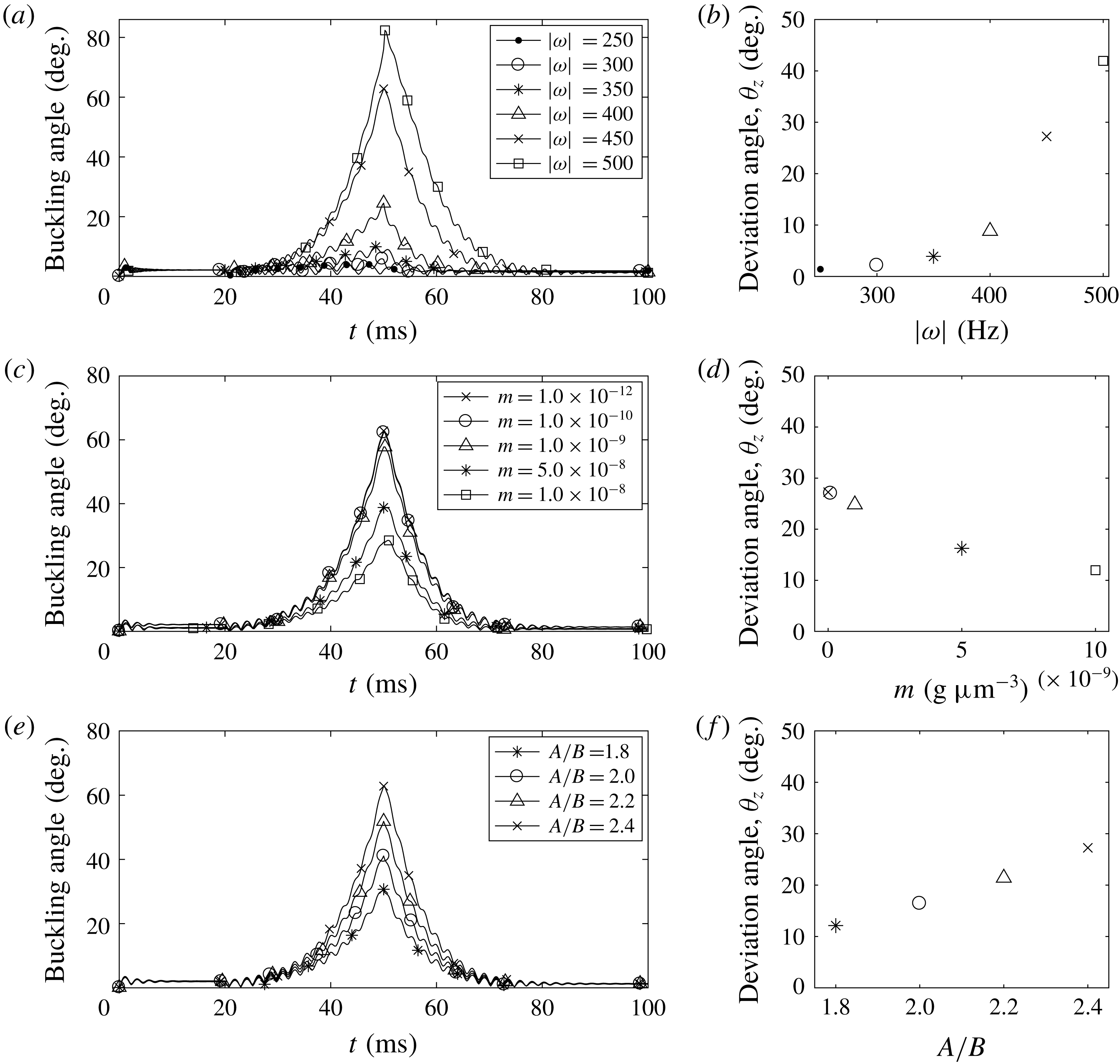
Buckling angle (a,c,e) and deviation angle (b,d,f) with various rotational frequencies of the motor
 $\unicode[STIX]{x1D714}$
(a,b), mass densities of the cell body
 $m$
(c,d) and the body ratios
 $A/B$
(e,f). The other parameters are the same as those in table 1.

Figure 11(a,b) shows buckling angles as functions of time (a) and the steady deviation angles (b) for various rotational frequencies of the motor. As the motor frequency increases above 350 Hz, the buckling angle and the steady deviation angle increase substantially. However, when the motor rotates at a rate below 350 Hz, the buckling and deviation angles are so small that the new swimming direction is almost aligned with the old swimming direction, although the hook buckles very slightly and is unstable, as observed in figure 11(a). Such small deviations might not be noticeable in experimental settings.
The buckling angle and the steady swimming direction also depend on the mass density of the cell body: see figure 11(c,d). As the mass density
 $m$
increases, since the total mass
 $M$
and the moment of inertial tensor
 $\unicode[STIX]{x1D644}_{0}$
increase, which makes it more difficult for the cell body to move and flick, both the maximum buckling angle and the steady deviation angle decrease. When the mass density is smaller than
 $m=10^{-10}~\text{g}~\unicode[STIX]{x03BC}\text{m}^{-2}$
, the buckling angle and the steady deviation angle remain almost the same. Since the total mass of a cell body can be considered as the sum of the mass of the fluid inside the cell body and the mass of its surface, its mass density is approximately 6–50 000 times larger than the surrounding fluid density based on the data in figure 11(c,d). One might think that these values are unrealistically large compared to the density of a real bacterium which is known to be slightly larger than that of water (Weng et al.
Reference Weng, Delgado, Son, Burg, Wasserman and Manalis2011; Lewis, Craig & Senecal Reference Lewis, Craig and Senecal2014). However, we find that the motion of the bacterium is independent of the mass density
 $m$
of the cell body when it is smaller than
 $10^{-11}~\text{g}~\unicode[STIX]{x03BC}\text{m}^{-2}$
. Especially, the run–reverse–flick movement of the bacterium is almost the same whenever
 $m$
is smaller than
 $10^{-11}~\text{g}~\unicode[STIX]{x03BC}\text{m}^{-2}$
.
Figure 11(e,f) shows that the maximum buckling angle (e) and the steady deviation angle (f) increase when the cell body ratio
 $A/B$
increases. Note that we change the ratio
 $A/B$
while the major axis
 $A$
of the ellipsoidal body is fixed as a constant. Thus, as the ratio
 $A/B$
increases, the short axis
 $B$
decreases, since the drag force on the cell body decreases, which makes it easier for the cell body to move and flick, the maximum buckling angle and the steady deviation angle increase.
4 Discussion and conclusions
We present a comprehensive model for a single-flagellated bacterium which includes an ellipsoidal cell body and a flagellum composed of an embedded motor, a compliant hook and an elastic helical filament. This mathematical model features: (i) the interaction between the cell body and the flagellum; (ii) the compliant hook that links the rotary motor to the filament working as a universal joint to transmit the motor rotation; (iii) the elastic helical flagellum inducing the translation–rotation coupling; and finally (iv) the interaction between the cell and its surrounding viscous fluid. Our model applies the motor-driven force alone to generate the helical wave propagation along the flagellum which results in the cell movement. We use Kirchhoff rod theory to model the elastic helical flagellum together with the hook and employ the penalty method to describe the dynamics of the rigid cell body. The hydrodynamic interaction between the fluid and the cell is represented by the regularized Stokes formulation.
Our simulation results on the average swimming speed and power efficiency of the cell, depending on the ratios of
 $l/A$
and
 $N_{\unicode[STIX]{x1D706}}$
, are comparable with those of the previous studies based on the resistive-force theory and the slender-body theory (Higdon Reference Higdon1979; Phan-Thien et al.
Reference Phan-Thien, Tran-Cong and Ramia1987) although there is a quantitative difference in power efficiency. In fact, this difference arises because the driving force in our model is applied only at the motor, as observed in nature, instead of rotating the whole flagellum as a rigid body, as done in the previous works. We further confirm that the aspect ratio of the cell body plays a significant role in determining the swimming speed and the counter-rotation rate of the cell body.
It is known that the helical filament of V. alginolyticus is intrinsically and permanently left-handed. This implies that, when the motor turns CCW, the helical wave propagates from the motor to the distal end of the filament and thus pumps the fluid away from the cell body, which results in the forward run. In contrast, when the motor turns CW, the helical wave propagates toward the motor and thus pulls the cell backward, which results in the backward run. In the absence of the buckling of the hook, the forward and backward runs of the cell in this work are consistent with the previous studies of rotating flagella even in the absence of the cell body (Kim et al. Reference Kim, Bird, Parys, Breuer and Powers2003; Lim & Peskin Reference Lim and Peskin2012; Park et al. Reference Park, Kim, Ko and Lim2017).
A monotrichous bacterium with a single left-handed helical flagellum can buckle and reorient by switching the rotational direction of the motor from CW to CCW, and the degrees of buckling and reorientation depend on the rotational frequency of the motor, elastic properties of the hook and physical and geometrical properties of the cell body. In particular, Euler’s beam theory evaluates a buckling condition with the fixed bending modulus of the hook and the hook length, and predicts a critical motor frequency that separates stable hooks from unstable ones. The critical threshold in theory, however, turns out to be different from the simulated critical motor frequency. One reason for this discrepancy is that, whereas the beam theory considers the axial and torsional loadings only, the hook in our model is clamped or hinged on the wall of the cell body that can freely move, and thus the load perpendicular to the axial direction might facilitate the hook’s buckling.
Variations in the physical and geometrical properties of the hook and the cell body demonstrate how these parameters affect the buckling angle and the new swimming direction after the buckling of the hook and the flick of the bacterium by measuring the buckling angle and deviation angle. Our simulation results show that the relaxed bending modulus affects the buckling angle much more than the twist and loaded bending moduli of the hook. This result is consistent with a previous study on rotating flagella (Park et al. Reference Park, Kim, Ko and Lim2017), in which the maximum buckling angle is inversely proportional to the bending modulus of the relaxed hook. The change of properties of the cell body also makes a significant difference in the buckling dynamics. For a heavier cell body, the cell turns with a lesser degree. For a more slender cell body, the cell turns with a larger degree, which may allow bacteria with a rod-shaped cell body to have more directional freedom than ones with a spherical cell body.
Acknowledgements
Y.K. was supported by National Research Foundation of Korea Grant funded by the Korean Government (grant no. 2017R1E1A1A03070636), and S.L. was supported by National Science Foundation grant no. DMS-1410886 and the Charles Phelps Taft Research Center at University of Cincinnati, USA.
Supplementary movies
Supplementary movies are available at https://doi.org/10.1017/jfm.2018.799.