Implications
There is considerable emphasis on improving fertility in dairy cows. However, the complexity of reproduction is such that predicting the importance of different factors (biology v. management) affecting reproductive performance is not straightforward. This study has developed a simulation model to do this, at individual cow and herd level.
Introduction
Over the last decades, the focus in dairy farming has been on improving milk yield (MY). This has worked remarkably well: MY has increased from 2500 kg milk/cow per year in the 1900s to 4000 kg milk/cow per year in the 1950s, to more than 8000 kg milk/cow per year at present (Capper et al., Reference Capper, Cady and Bauman2009). This higher milk production has had multiple implications: the modern cow needs more resources (food, water), and has become more susceptible to disease and metabolic problems (Alban et al., Reference Alban, Agger and Lawson1996). In addition, fertility traits have been found to be negatively correlated with milk production both genetically and physiologically, and the number of herds that experienced problems with fertility increased (Pryce et al., Reference Pryce, Coffey and Brotherstone1999; Oltenacu and Broom, Reference Oltenacu and Broom2010).
Given the fact that impaired fertility decreases both economic value and longevity of the dairy cow, a lot of emphasis has been placed on improving fertility in recent decades. A number of mechanisms linked to impaired fertility have been uncovered, like the link between negative energy balance (EB) and the hormonal status of the cow (Wathes et al., Reference Wathes, Fenwick, Cheng, Bourne, Llewellyn, Morris, Kenny, Murphy and Fitzpatrick2007; Fenwick et al., Reference Fenwick, Fitzpatrick, Kenny, Diskin, Patton, Murphy and Wathes2008), or risk factors for prolonged postpartum anestrous (ANST) (Ledoux et al., Reference Ledoux, Touze, Richard, Ponter, Bosc and Grimard2011; Crowe et al., Reference Crowe, Diskin and Williams2014).
However, it is nearly impossible on-farm to detect the underlying physiological mechanics from the outside and as such, the cow is a ‘black box.’ In order to better understand why cows are not getting pregnant, one would have to take, in a large population of cows and different environments (i.e. nutritional, management), a whole spectrum of measurements during a long period of time. This is expensive and labor-intensive, and not realistic, even in research farms. A way to overcome this problem is by using a simulation model that is able to integrate knowledge from literature, to simulate events during the lifetime of a cow and link these events to changes in the physiological status of the cow. A simulation model can be used to evaluate long-term effects of impaired fertility on productive performance (for instance the ‘cost’ of 1% embryo mortality). In order to realistically simulate an individual cow’s reproductive performance during lifetime, it is necessary to include reproductive management rules. If the individual cow model can be expanded to herd level by introducing management rules, it will become possible to test different scenarios using different reproductive management strategies.
Accordingly, this paper introduces a dynamic simulation model that aims to simulate productive and reproductive performance of a cow during her lifetime. We hypothesized that a simple compartment model of the reproductive function could adequately describe typical dynamics of reproductive performance and deviations in reproductive trajectories along the different physiological stages of the cow reproductive cycle (anovulatory (ANOV), cycling and pregnant). It thus could provide the basis for evaluation of the relative importance of different factors affecting fertility at individual cow level. The model, as an individual component, is embedded in a computing architecture that allows description of farm-management rules. This tool was designed to be suitable for use in simulating herd-level responses to different farming systems.
Material and methods
Model description: cow level
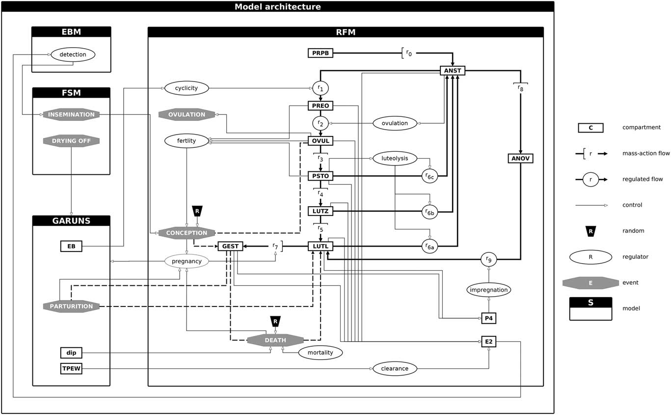
The cow model consists of two parts: an existing productive function model (GARUNS; part one) which is linked to a new reproductive function model (RFM; part two) (Figure 1). The cow model can be expanded to herd level by linking GARUNS and RFM to a farming system model (FSM) as described in the next section. Communication between models is ensured through discrete events: ‘insemination’ and ‘drying-off’ individually triggered by FSM; ‘parturition’ generated by GARUNS; ‘ovulation,’ ‘conception’ and ‘death’ (of embryo or fetus) generated by RFM.
Cow model diagram. EBM=estrous behavior model; FSM=farming system model; EB=net energy balance; dip=days in pregnancy; TPEW=total processed energy per weight; RFM=reproductive physiology model; competence stages: PRPB=prepubertal; ANST= anestrous; ANOV=anovulatory; PREO=pre-ovulating; OVUL=ovulating; PSTO=post-ovulating; LUTZ=luteinizing; LUTL=luteal; E2=estradiol; P4=progesterone. GEST=gestant.

Part one: productive function model
The GARUNS model simulates individual productive performance of a dairy cow throughout her lifespan (see detailed description in Martin and Sauvant, Reference Martin, Blanc, Agabriel, Disenhaus, Dupont, Fréret, Elis, Gatien, Salvetti and Friggens2010a and Reference Martin, Friggens, Dupont, Salvetti, Fréret, Rame, Elis, Gatien, Disenhaus and Blanc2010b). This animal model has been calibrated to simulate Holstein dairy cows. GARUNS consists of the coupling of a regulating and an operating sub-model. The regulating sub-model describes the dynamic partitioning of a dairy cow’s priorities between life functions: growth (G), ageing (A), balance of body reserves (R) and nutrient supply of the unborn (U), newborn (N) and suckling (S) calf. The operating sub-model calculates on a daily time-scale changes in BW and composition, fetal growth, MY and composition and dry matter intake (DMI) in dairy cows throughout their lifespan. In the GARUNS model, genetic-scaling parameters make it possible to scale individual performance and simulate differences within and between breeds (Martin, Reference Martin2009). In order to link with RFM, the GARUNS model was adapted to take into account pregnancy interruptions, and two synthetic variables of animal energetic status have been added: TPEW, the daily total processed metabolizable energy per kilogram of weight in MJ/day per kilogram (TPEW=(I+C X )/W, where I is the energy intake, C X the energy from labile body mass catabolism and W the non-labile body mass) and EB, the daily net metabolizable energy balance (EB=I−M−Y−P−AW, where I is the energy intake, M the maintenance energy requirement, Y the milk energy requirement, P the pregnancy energy requirement and AW the energy for non-labile mass growth). The two variables TPEW and EB are intended to provide regulating factors to RFM based on energy metabolism (see the ‘Part two: reproductive function model’ section).
Part two: reproductive function model
Reproductive function model is derived from a conceptual modeling framework of reproductive physiology (Martin et al., Reference Martin and Sauvant2012) and was designed to be linked to the GARUNS model and to incorporate genetic, endocrine, metabolic and stochastic regulating components of fertility.
Reproductive function model describes the basic steps in reproduction during the lifespan of a cow: commencement of puberty, ovarian cyclicity and pregnancy. Reproductive function model provides the times of start of gestation and interruption owing to embryonic or fetal death to the GARUNS model.
The reproductive system is modeled by way of a cyclic compartmental system (Figure 1) composed of nine competence stages defined to represent changes in reproductive dynamics over lifetime: prepubertal (PRPB), ANST, ANOV, pre-ovulating (PREO), ovulating (OVUL), post-ovulating (PSTO), luteinizing (LUTZ), luteal (LUTL) and gestating (GEST). The term competence stage refers to the idea that each stage has a specific physiological ability that contributes to the whole behavior of the reproductive system. The model was initialized with PRPB=0.999 and ANST=0.001, so that the sum of competence stages is always equal to 1. Flows between competence stages represent changes in the current reproductive status of the cow. The dynamics of competence stages for one cow over different time scales are shown in Supplementary Figures S1 to S3. The transition from PRPB to ANST represents the start of reproductive activity at puberty. The cyclic path through ANST, PREO, OVUL, PSTO, LUTZ, LUTL forms the regime of ovulatory cycles, although ANOV and GEST are transient stages that interrupt this regime. Anovulatory is a stage that refers explicitly to ovarian dysfunctioning that interrupts ovulations (i.e. interrupted cyclicity), whereas ANST is a pivotal stage of looping within ovulatory cycles (see Figure 1).
This dynamic system evolving through competence stages is used to generate estradiol (E2) and progesterone (P4) hormonal profiles. The dynamics of P4 and E2 for one cow over different time scales is shown in the Supplementary Figures S4 to S6.
Transitions between competence stages are controlled by regulating variables that trigger shifts from PRPB stage to ANST stage (puberty) and then to stages belonging to the ovulatory cycling loop, from ovulatory cycling stages to pregnancy (fertility and pregnancy), and from postpartum or post-abortive ANST stage back to the ovulatory cycling loop stages (cyclicity). In addition, the variable impregnation controls recycling from the ANOV stage, and the variable clearance controls the intensity of E2 signal (Figure 1).
The variable puberty depends on the genetic parameter v B, which determines the age of the cow at first ovulation. The variable fertility depends on a genetic-scaling parameter v I (threshold of fertilization probability), a linear combination of competence stages PREO, OVUL and POST (defining the width of the window for fertilization) and a random component that determines if fertilization is successful in the fertility window. This concept of fertility window is shown in the Supplementary Figure S7. The variable pregnancy is Boolean, shifting from 0 to 1 at event ‘conception’ and from 1 to 0 at event ‘parturition’ or ‘death’ (embryonic or fetal). The variable cyclicity depends on GARUNS output EB (as net EB blocks cycling when highly negative), the variable impregnation depends on the intensity of P4 signal (an extended period of low P4, for instance due to prolonged negative EB, delays recycling after parturition or abortion) and the variable clearance depends on GARUNS output TPEW (high levels of energy metabolism increase clearance of E2).
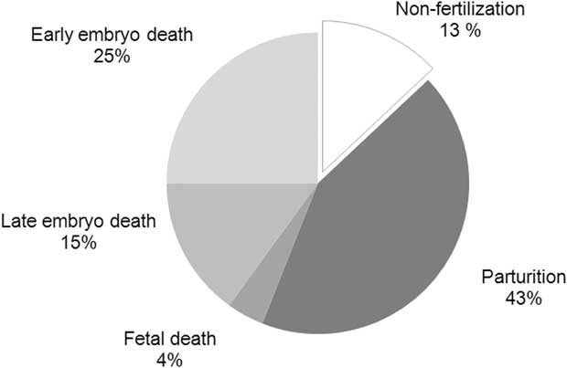
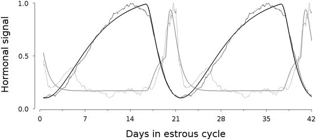
The event ‘ovulation’ is triggered when OVUL is the maximum competence stage, that is, when OVUL > {PRPB; ANST; PREO; PSTO; LUTZ; LUTL; GEST}. This event remains an internal signal and is only used to compute inter-ovulatory intervals. The event ‘conception’ is triggered 24 h after event ‘insemination’ if fertilization succeeds and the event ‘death’ is triggered randomly with a daily probability defined for three periods of pregnancy (days 1 to 16: early embryo death with probability 0.0230, days 16 to 45: late embryo death with probability 0.0096 and day 45 to term: fetal death with probability 0.0004). These probability values were derived from the results of a sensitivity analysis to obtain realistic mortality rates (Figure 2). Other model parameters are fractional rates that control transitions between competence stages (n=10 parameters) and hormonal signal release and clearance (n=4). These parameters were estimated by fitting to produce E2 and P4 dynamics over the estrous cycle consistent with reference profiles derived from a compilation of literature data (Martin et al., Reference Martin and Sauvant2013; Figure 3). The EB threshold parameter B controls the variable cyclicity and determines the level of negative net EB that blocks cycling. After preliminary tests on the variability of reproductive intervals, the value of B was set to an average working reference (B=−10 MJ metabolizable energy/day), potentially modifiable to modulate reproductive timing. A detailed description of the RFM system of differential equations, variables and flows, events and parameters is provided in the Supplementary Tables S1 to S4.
Distribution of the fate of 100 527 inseminations of 10 000 simulated cows over a standard 5000 days lifetime period.

Hormonal signal dynamics for estradiol and progesterone over two estrous cycles in dairy cows (respectively in gray and black; model simulations in thick line and literature-based reference profiles from Martin et al., Reference Martin and Sauvant2013 in thin line).

Model description: herd level
Animal models based on the coupling of GARUNS and RFM are individualized in a computing architecture allowing multiple simulations at cow level, creating a herd of individual virtual cows. At the start of the simulation, it is possible to create a herd with given age distribution and given genetic-scaling parameter distributions. The FSM was designed to describe a farm protocol of heat detection, insemination, feeding (amount and energy density), drying-off and culling, based on herd management rules. In addition, a simple estrous behavior model (EBM) has been developed to convert the E2 signal generated by RFM into a probability of estrous detection provided to FSM. In case of detection, the event ‘insemination’ is sent to RFM and triggers the fertilization test. Farming system model and EBM are described in the Supplementary Material S1.
Introducing variability in the model
In the GARUNS model, the term genetic-scaling parameter refers to a parameter intended to scale the level of performance of an individual cow and thus to be considered as a proxy for genetic potential for a given trait. In practice, by changing these parameters, the productive performance of one cow can be adjusted. At herd level, these parameters are drawn from random normal distributions and play the role of generators of between-cow variability (the random processes of trigger for conception and embryonic/fetal death introduce between-reproductive cycle variability). The GARUNS genetic-scaling parameters are proxies for mature body size, body fatness, reserve liability, maternal reserve reproductive investment, milk potential, milk fat and protein contents and intake capacity. Previous works have shown the ability of these parameters to fit individual cow performance (Phuong et al., Reference Phuong, Blavy, Martin, Schmidely and Friggens2015a and Reference Phuong, Martin, de Boer, Ingvartsen, Schmidely and Friggens2015b; Gaillard et al., Reference Gaillard, Martin, Blavy, Friggens, Sehested and Phuong2016). Random distributions of the GARUNS genetic-scaling parameters used in this paper were derived from these studies and first explorations of the model behavior (Martin, Reference Martin2009).
Consistent with the GARUNS model logic, three so-called genetic-scaling parameters were incorporated into RFM: v I , the threshold of fertilization probability (as a proxy for fertilization rate), v B , the puberty index (as a proxy for age at first ovulation) and v Z , the speed of ovarian dynamics (as a proxy for number of follicular waves and thus estrous duration). The average values and standard deviations of genetic-scaling parameters v I , v B and v B were defined to obtain respectively a mean fertilization rate of 97% (range 70% to 100%), a mean age at puberty of 8 months (range 5 to 11) and a mean estrous length of 21 days (range 19 to 24). The Supplementary Table S5 provides reference values and random distributions of genetic-scaling parameters of RFM and GARUNS.
Model simulation
The model was implemented in C++. The discrete event system was implemented by extending the DEVS formalism (Discrete EVent system Specification for modeling and analyzing general systems; Zeigler, Reference Zeigler1976). In brief, events were organized into a timetable, and the model was integrated by consecutive time slices until the occurrence of the first event that may affect the status of the cow. Numerical integration of differential equations was done with the fourth order Adams–Bashforth–Moulton solver of the boost::odeint library, with an integration step of 0.1 day for GARUNS and 15 min for RFM. Random number generation was performed by using the std::default_random_engine library and associated distributions of the GNU Compiler Collection (GCC 6), seeded with current time.
Results presented in this paper are focused on animal level and are based on a series of 10 000 simulations of individual cows over 5000 days lifetime period, with the 11 genetic-scaling parameters being randomly drawn together at simulation start (see Supplementary Table S5) and with a standard context of management for feeding, insemination and drying-off. This context is assumed to represent a healthy herd, with 100% of estrus detected, artificially inseminated with quality semen. All cows were born at t=0 and fed indoor ad libitum along their lifetime with a standard constant diet (60% DM and 12.3 MJ/kg DM intake content). The model was run without culling rules, without voluntary waiting periods after calving, with insemination starting from the age of 15 months, without limitation of the number of insemination until conception and with drying-off when days in milk≥300 and days in pregnancy≥219 or when days in milk≥300 and MY≤5 kg/day). Simulated data were analyzed using Scilab to compute productive and reproductive performance statistics by reproductive cycle (from birth to first parturition for parity 0 and from parturition n to n+1 for parity n>0). Within each cow, reproductive intervals were calculated for each reproductive cycle between event times: estrous cycle length (i.e. ovulation without conception to next ovulation), parturition to first ovulation, parturition to conception with completed gestation, calving interval and gestation length. Within-cow reproductive rates were calculated for each reproductive cycle using ratios of event counts: insemination rate is the number of inseminations divided by the number of ovulations; non-fertilization rate is the number of fertilization failures divided by the number of inseminations; early and late embryo and fetal death rates are the number of early and late embryo and fetal deaths divided by the number of inseminations; and parturition rate is the number of parturitions divided by the number of inseminations.
Results
Table 1 presents the descriptive statistics for the 10 000 simulations for parity 0, 1 and 2 and more. As cows in parity 0 have never calved or been milked, MY and postpartum values are not determined and the reproductive intervals for parturition to ovulation, parturition to conception and parturition to parturition are defined from birth of the cow. The average estrous length is 21 days, the average age at first calving is 25.9 months and the average gestation length is 282.5 days. The 90% confidence interval for parturition to ovulation interval is (38 to134) days which is longer than the ranges reported in literature (e.g. (15 to 80) days in Canfield et al., Reference Canfield, Sniffen and Butler1990). Cows in parity 1 start cycling, on average 30 days sooner than cows of parity 2 and older. This result is due to the simulated longer period of negative EB in multiparous cow and suggests that the EB threshold parameter controlling the resumption of cyclicity should be adjusted to reduce parturition to ovulation intervals. The 90% confidence interval for calving interval is (332 to 623) days which is again about 30 days longer than the ranges reported in literature (e.g. (300 to 600) days in Pryce et al., Reference Pryce, Nielsen, Veerkamp and Simm2000). More details on the behavior of the model compared with literature data are provided in the Supplementary Figures S8 to S18 and concern growth and body condition score (BCS) over lifetime, BW, MY and DMI over lactation, fetal growth over gestation, calf birth weight, gestation length and calving interval.
Descriptive statistics by parity of productive and reproductive performance of the 100 527 reproductive cycles completed by 10 000 simulated cows

nd=not determined; TPEW=total daily processed metabolizable energy per kg weight; EB=net metabolizable energy balance.
1 Parity=5.7±2.5.
2 TPEW=(I+C X )/W, where I is the energy intake, C X the energy from labile body mass catabolism and W the non-labile body mass (GARUNS model variables).
3 EB=I−M−Y−P−A W , where I is the energy intake, M the maintenance energy requirement, Y the milk energy requirement, P the pregnancy energy requirement and A W the energy for non-labile mass growth (GARUNS model variables).
4 Postpartum BW and body condition score are recorded just after calf and annexes expulsion.
5 Inter-ovulatory interval considering only ovulation without conception.
6 For parity 0, the birth of the cow is used instead of parturition and intervals correspond to ages at 1st ovulation, 1st conception and 1st parturition.
7 Considering only conception with completed gestation.
The fate of the inseminations performed during the 10 000 simulations (100 527 inseminations in total) is displayed in Figure 2. In total, 13% of inseminations does not result in fertilization and 87% lead to fertilization, with 25% resulting in early embryonic death (0 to16 days after insemination), 15% in late embryonic death (16 to 45 days after insemination), 4% in fetal death (over 45 days after insemination and before parturition) and 43% in on-term parturition. These results are consistent with values reported in literature (Fréret et al., Reference Fréret, Ponsart, Rai, Jeanguyot, Paccard and Humblot2006; Sartori et al., Reference Sartori, Bastos and Wiltbank2010; Walsh et al., Reference Walsh, Williams and Evans2011; Diskin et al., Reference Diskin, Parr and Morris2012): non-fertilization between 5% and 17%, early embryonic mortality between 23% and 35%, late embryonic mortality between 4% and 24% and fetal mortality between 8% and 9%. Overall, insemination success rates (recalving rates) have been reported between 41.3% and 45.5% over the 1999 to 2008 period within the French Holstein breed (Le Mézec et al., Reference Le Mézec, Barbat-Leterrier, Barbier, Gion and Ponsart2010). This is consistent with the outcomes of our simulations.
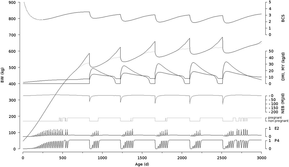
One of the main features of the model is its ability to generate P4 and E2 profiles consistent with reference profiles from literature (P4: RMSE=0.02, E2: RMSE=0.04, dimensionless (0 to 1); Figure 3). Figure 4 shows the simulation of one cow over 3000 days, with both productive and reproductive information. The upper line shows the fluctuations in BCS. The first part of the line is dashed because the formula used to compute BCS has not been specifically validated for young stock. The second line from the top shows the fluctuations in BW. The black line shows BW including the weight of the gravid uterus; the gray line shows BW excluding the gravid uterus. The third, fourth and fifth lines show DMI, MY and EB, respectively. The sixth line shows whether the cow is pregnant or not, thus giving an overview of the number of early or late embryonic or fetal deaths. The seventh and eighth lines show the E2 and P4 profiles. If there is embryonic or fetal death, the P4 profile shows a prolonged LUTL phase. Supplementary Figures S19 and S20 show two simulations of very extreme cows (lowest v. highest calving interval within the 10 000 simulated cows).
Model simulation over 3000 days lifetime for an individual cow (individual closest to the average of the 10 000 series). BCS=body condition score; DMI=dry matter intake; MY=milk yield; NEB=net energy balance; E2=estradiol, P4=progesterone.

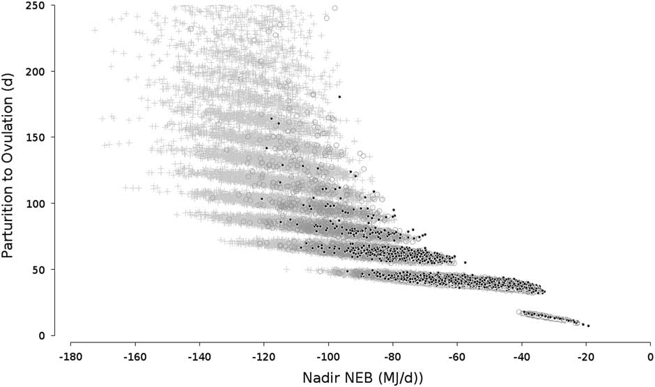
Figure 5 illustrates the interacting effects of two model properties. First, the effect of negative EB that transiently blocks the return to ovarian cyclicity after parturition can be seen by the overall increase of parturition to ovulation intervals with decreasing levels of EB. Second, in situations where longer time is required until recycling (associated with low EB), the system is exposed to a longer period of low P4 impregnation. This effect can shift the cow to a prolonged ANOV stage, which is represented by the occurrence of extreme parturition to ovulation intervals (1% of intervals above 241 days). This way, the model mimics interruptions of cyclicity and generates low-fertility cows. In real situations, these cows are not maintained in the herd but treated or culled. As also shown in Table 1, first parity cows start cycling sooner after calving. The grouping by strata of data points is due to the 21-day interval between cycles that cadence the model.
Parturition to first ovulation interval (days) according to nadir net energy balance (MJ/day) over 90 527 simulated dairy cow reproductive cycles for parity 1 (black dot), 2 (gray circle) and 3 and more (gray plus).

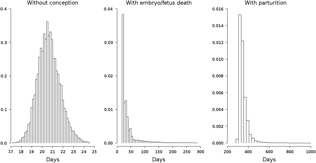
Figure 6 shows the distributions of inter-ovulatory intervals without conception (A), with conception and embryonic/fetal death (B) and with conception and parturition (C).
Distributions of dairy cow inter-ovulatory intervals: without conception (left panel), with conception followed by embryo or fetus death (middle panel) and with conception going to parturition (right panel) (over 529 211 ovulations). The data in right panel represent the durations from the estrus at which conception occurred to the first estrus following the subsequent parturition.

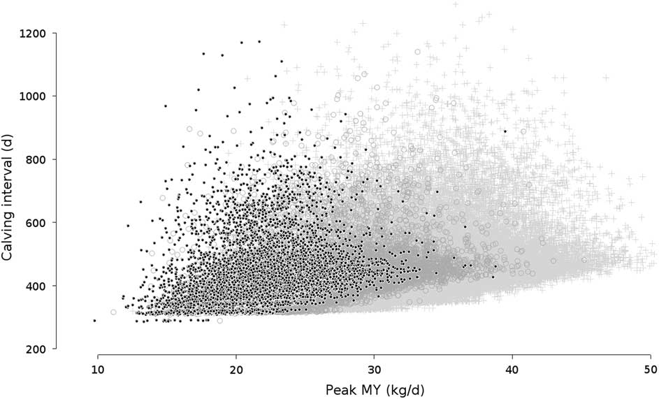
Figure 7 shows the relationship between MY and calving interval for parity 1, parity 2 and parity 3 and older. This graph is an example of how the combination of different effects increases variability in the model. First, MY is correlated with nadir EB, meaning that higher yielding cows have a higher chance of prolonged postpartum ANST, and thus calving interval. Second, higher MY is responsible for higher clearance of hormones from blood, decreasing the chances of an estrus being detected. The random generators for fertilization and embryonic/fetal death increase variability even more. The occurrence of extremely long calving intervals concerns animals cumulating long ANST periods, insemination failures and repeated embryonic/fetal deaths (6% of calving intervals above 600 days). As mentioned above, in real situations these cows would have been removed from the herd.
Calving interval (days) according to peak milk yield (MY, kg/day) over 90 527 simulated reproductive cycles of dairy cows for parity 1 (black dot), 2 (gray circle) and 3 and more (gray plus).

Discussion
The purpose of the study was to build a realistic model of reproductive functioning and thereby to allow prediction of lifetime performance by combining it with the GARUNS model. This purpose has been achieved and reproductive performance are globally consistent with literature data. Next steps would be to conduct detailed behavioral and sensitivity analyses of the model in order to evaluate the model against broader data, refine parameter values and improve the realism of simulations.
The reproductive axis is a complex system which involves a hormonally-based sequential coordination of biological units (hypothalamic–pituitary complex, ovarian oocytes, follicles and corpora lutea, inseminated spermatozoa, zygote–embryo–fetus–calf stages, maternal uterus, placenta and udder), supporting and promoting the fate of an immature ovum to become a viable calf. There is an increasing corpus of knowledge on the functions of each of these elementary components and the hormonal signals providing communication between them. The neuroendocrine-mediated LUTL regression is one example where considerable research efforts have been carried out (McCracken et al., Reference McCracken, Custer and Lamsa1999). There are also numerous experimental observations at an animal scale that have led to hypotheses on the effects of management, genetics, nutrition, metabolism, productive performance and body condition on reproduction (Walsh et al., Reference Walsh, Williams and Evans2011). Still, there is no clear consensus on the links between the underlying physiological mechanisms that are impacted by these factors which alter reproductive function and cause poor fertility in dairy cattle.
What we do know is the sequence of reproductive events whose consecutive successes lead a cow from one calving to the next, including: (1) calf delivery, placental expulsion and uterine involution, (2) postpartum recovery of the endocrine function of the hypothalamic–pituitary complex and resumption of ovarian cyclicity, (3) ovulation of a quality oocyte, estrus expression and luteinization, (4) insemination and fertilization, (5) endometrial implantation, maternal recognition of pregnancy and placentation, (6) embryo survival and fetal normal development and (7) maturation of the fetal corticotropic axis and triggering of parturition. What we do not know is the impact of a deviation occurring at a specific point on the subsequent steps.
Another unknown factor is how other biological systems, such as the digestive, metabolic and endocrine ones, intimately interact with the reproductive dynamic machinery. For instance, although it has been shown that negative EB decreases fertility, the hypothesis of a competition for energy between lactation and gestation in modern dairy cows selected for high milk production does not seem plausible given the very low-energy requirements to ovulate and initiate a reproductive cycle (Leroy et al., Reference Leroy, Opsomer, Van Soom, Goovaerts and Bols2008a). Although negative effects of fatty acids in follicular fluid, and also of adipokines, have been shown on oocyte viability (Leroy et al., Reference Leroy, Opsomer, Van Soom, Goovaerts and Bols2008a and Reference Leroy, Van Soom, Opsomer, Goovaerts and Bols2008b; Dupont et al., Reference Dupont, Scaramuzzi and Reverchon2014), it is much less clear how the physiological mechanisms driving the cow’s reproductive dynamics are affected by EB (Grala et al., Reference Grala, Lucy, Phyn, Sheahan, Lee and Roche2011). In the end, we still do not know if modern dairy cows are inherently less fertile as they are more productive or if dysfunctions in fertility are a consequence of their underlying high-energy metabolism.
Several authors, such as Garnsworthy et al. (2008) and McNamara and Shields (2013), have stressed the necessity of a systemic view of the animal for tackling the fertility issue, that is, a broader view of the relationships between life functions. In this context, modeling is a way to think about the fertility issue by formalizing the basic elementary components of the reproductive axis and make them interact dynamically with performance trajectories to simulate a real cow. Several models have already been developed in the field of dairy cow reproduction. Existing works are generally focused on a specific part of the reproductive process, like the estrous cycle (Boer et al., Reference Boer, Röblitz, Stötzel, Veerkamp, Kemp and Woelders2011), the hypothalamic–pituitary–gonadal axis (Clément, Reference Clément and Monniaux2016) or follicular selection (Clément and Monniaux, Reference Clément2013). Other existing models consider reproduction as a succession of stochastic stages and are based on an aggregation of equations (Brun-Lafleur et al., Reference Brun-Lafleur, Cutullic, Faverdin, Delaby and Disenhaus2013). A first attempt to connect a reproductive model to the GARUNS model of productive performance has already been published (Phuong et al., Reference Phuong, Blavy, Martin, Schmidely and Friggens2015a). This model uses an empiric function that calculates the likelihood of conception of a viable calf, but without explicit representation of the elementary steps of the reproductive process. The present model is a step toward a systemic representation of the reproductive function, allowing the decomposition into elementary effects (genetic determinism, endocrine and metabolic control and stochastic occurrence of events conception and embryonic/fetal death). Genetic determinism was assumed to impact: the precocity of reproductive maturity, the velocity of ovarian dynamics and the ability to be fertilized. Scaling these components for individual cows creates the possibility to generate individual variability in the timing and frequency of ovulations and conceptions. It also creates the opportunity of controlling the basal genetic level of fertilization independent of the other components of fertility. Endocrine control by P4 impregnation is based on the assumption that the reproductive machinery needs certain levels of P4 to be fully operational. In this way, low P4 levels at the start of recycling can negatively impact fertility. Metabolic control of RFM by the GARUNS model is decomposed into two effects within two steps of the reproductive cycle: negative EB was assumed to delay postpartum ANST (Aungier et al., Reference Aungier, Roche, Diskin and Crowe2014) and the level of energy metabolism (increasing with genetic milk potential) was assumed to increase E2 clearance (Sangsritavong et al., Reference Sangsritavong, Combs, Sartori, Armentano and Wiltbank2002), thus muting heat expression. A correlation between high MY and length of the calving interval, as seen in Figure 7, emerges with these two effects applied to animals with various genetic profiles experiencing various energy metabolisms. Thus, these two assumed effects appear at first sight to be sufficient to describe the decline in fertility in modern high-producing dairy cows. In the model, the occurrence of embryo/fetus mortality is a stochastic component and has no relationship with animal or reproductive management factors. Any mechanistic representation of the determinism of death during gestation would require assumptions at a finer level of biological organization. The only assumption that was implemented is related to the cutting of gestation in three stages with decreasing probabilities of mortality. The model thus explicitly distinguishes non-fertilization from early mortality. The model can, therefore, be used to estimate the long-term effect of deviations in reproductive performance on productive performance. For instance, our simulations showed that a decrease in 1% of embryo/fetus mortality induces a decrease in 174 kg MY over a 5000days-lifetime. This result illustrates the potential use of the model for economic interpretation of fertility dysfunctions.
The modular structure of the model makes it a useful tool to implement and test various hypotheses, such as a theoretical genetic correlation between genetic-scaling parameters of milk potential and fertility or embryo mortality. At the herd level, the model could be used to simulate and compare farming systems combining genetic, feeding and breeding options. In the field, there is a potential use of this model in the context of precision farming to control deviations from the expected performance trajectories.
Conclusions
The model presented in this paper allows simulation of fertility together with a productive performance at the animal and herd level. This dynamic model combines genetic, endocrine, metabolic and stochastic effects at the scale of the reproductive axis and allows testing effects of changes in reproductive or feeding management strategies. It generates realistic outputs in terms of productive and reproductive performance. The model can easily be manipulated and used as a tool to help to disentangle the underlying components within the fertility process of a cow. It could also be used for evaluating different reproductive management scenarios.
Acknowledgments
The authors would like to acknowledge Henri Woelders, Nicola Dennis and Susanne Meier for sharing their expertise on genotype-environment effects on reproduction, and the INRA PHASE Cowplaner group for initial discussions on reproductive physiology. The authors would also like to acknowledge the European Union for funding this project. This study was performed as a part of the European Project Pluridisciplinary study for a RObust and sustainabLe Improvement of Fertility In Cows (PROLIFIC, grant no. FP7.KBBE.2012.6, grant agreement no. 311776).
Declaration of interest
None.
Ethics statement
None.
Software and data repository resources
None of the described models were deposited in an official repository.
Supplementary material
To view supplementary material for this article, please visit https://doi.org/10.1017/S1751731118001830