1 Introduction
The freezing of soils and particulate suspensions has received increasing attention in recent years owing to its relevance to geophysical phenomena (Dash, Rempel & Wettlaufer Reference Dash, Rempel and Wettlaufer2006; Wettlaufer Reference Wettlaufer2019), water purification (Gay & Azouni Reference Gay and Azouni2002; Gao, Smith & Li Reference Gao, Smith and Li2006) and materials science applications (Deville et al. Reference Deville, Saiz, Nalla and Tomsia2006; Henderson et al. Reference Henderson, Ladewiq, Haylock, MacLean and O’Connor2013; Deville Reference Deville2017). In this process, ice is grown into a matrix of particles in water which may also contain dissolved salts and dispersants. For a range of freezing conditions and physical parameters, the ice segregates from the particle matrix, self-organizing into a variety of patterns (Taber Reference Taber1929; Qian & Zhang Reference Qian and Zhang2011; Deville Reference Deville2017). Material scientists exploit this phenomenon to create novel microstructured and biomimetic materials (Deville Reference Deville2013; Henderson et al. Reference Henderson, Ladewiq, Haylock, MacLean and O’Connor2013). When soils freeze, the ice tends to segregate into a sequence of approximately planar horizontal layers called ice lenses (Taber Reference Taber1929; Dash et al. Reference Dash, Rempel and Wettlaufer2006). While it is known that frost heave (the uplift of the soil surface in winter) is caused by the formation of ice lenses, the physical mechanisms governing their initiation and growth have yet to be fully explained (O’Neill Reference O’Neill1983; Rempel Reference Rempel2010; Peppin & Style Reference Peppin and Style2013; Wettlaufer Reference Wettlaufer2019). In soils with a high clay content, ice lenses can become non-planar, forming complex polygonal and reticulate vein structures (Taber Reference Taber1929; Mackay Reference Mackay1974; Arenson et al. Reference Arenson, Xia, Sego and Biggar2006; Peppin, Elliott & Worster Reference Peppin, Elliott and Worster2006; Deville Reference Deville2013; El Hasadi & Kodadadi Reference El Hasadi and Kodadadi2015; Wang et al. Reference Wang, You, Wang, Wang and Lin2016; Xu et al. Reference Xu, Yu, Yan and Tan2016; You, Wang & Worster Reference You, Wang and Worster2018b). In addition, most soils and colloidal suspensions contain dissolved solutes in the pore fluid, which significantly influence the freezing process (Hallet Reference Hallet1978; Chamberlain Reference Chamberlain1983; Arenson et al. Reference Arenson, Xia, Sego and Biggar2006; Pekor Reference Pekor2014; Schollick et al. Reference Schollick, Style, Curran, Wettlaufer, Dufresne, Warren, Velikov, Dullens and Aarts2016; Wang et al. Reference Wang, You, Wang, Wang and Lin2016; You et al. Reference You, Wang, Wang, Wang, Lia and Lin2018a; Dedovets et al. Reference Dedovets, Monteux and Deville2018; Ginot et al. Reference Ginot, Lenavetier, Dedovets and Deville2019).
In the present work, a model of an ice lens growing in a saline porous medium is developed and a linear stability analysis is undertaken. A characteristic equation is obtained giving critical conditions for the onset of unstable lens growth, and a diagram is constructed illustrating parameter regimes in which molecular diffusion or viscous flow controls the instability. The diagram indicates that dissolved impurities have significant effects on the growth and stability of ice lenses at the solute concentrations typically found in soils and freeze-casting applications. The results are applied to frost heave experiments on a silty clay soil (Konrad Reference Konrad1990) and a glass powder medium (Watanabe, Muto & Mizoguchi Reference Watanabe, Muto and Mizoguchi2001; Watanabe Reference Watanabe2002).
2 Ice lens growth in saline porous media
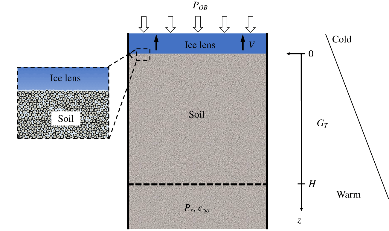
The system to be studied, shown in figure 1, consists of a solidification cell containing a column of soil freezing from the top down. The soil is made up of solid particles, and the pore fluid is composed of water and a dissolved solute. At the soil surface  $z=0$ is a planar ice lens that is growing without entering the soil pores (primary frost heave); an overburden pressure
 $P_{OB}$ acts on the top of the ice lens, so that the ice pressure is
 $p_{i}=P_{OB}$. Supplying the soil at position
 $z=H$ is a fluid reservoir at pressure
 $p_{r}$ and solute concentration
 $c_{\infty }$. Pressures are defined relative to atmospheric (gauge), so that
 $p_{r}=0$ for a reservoir at atmospheric pressure. A linear temperature gradient is imposed on the system, and a constant freezing speed
 $V$. This can be achieved by ramping the temperatures at the top and base (Penner Reference Penner1986; Konrad Reference Konrad1989a) or by moving the soil at speed
 $V$ through a fixed temperature gradient (Watanabe & Mizoguchi Reference Watanabe and Mizoguchi2000; Peppin, Wettlaufer & Worster Reference Peppin, Wettlaufer and Worster2008; Anderson & Worster Reference Anderson and Worster2014; Schollick et al. Reference Schollick, Style, Curran, Wettlaufer, Dufresne, Warren, Velikov, Dullens and Aarts2016; You et al. Reference You, Wang, Wang, Wang, Lia and Lin2018a; Saint-Michel et al. Reference Saint-Michel, Georgelin, Deville and Pocheau2019). At steady state the ice lens growth speed
 $V_{il}$ is equal to
 $V$.
Schematic diagram of a directional solidification cell containing a saturated soil with an ice lens at  $z=0$ and a reservoir at
 $z=H$. The reservoir contains pore fluid at pressure
 $p_{r}$ and solute concentration
 $c_{\infty }$. The ice lens is growing at speed
 $V$ within a fixed temperature gradient
 $G_{T}$ under an overburden pressure
 $P_{OB}$.

2.1 Governing equations
In the following the density differences between ice, water, particles and solute are neglected. The equations describing the system can then be written, in a frame of reference moving with the freezing speed  $V$, as
 $$\begin{eqnarray}\displaystyle & T=T_{0}+G_{T}z\quad (z>0), & \displaystyle\end{eqnarray}$$
 $$\begin{eqnarray}\displaystyle & \displaystyle \frac{\unicode[STIX]{x2202}p}{\unicode[STIX]{x2202}t}-V\frac{\unicode[STIX]{x2202}p}{\unicode[STIX]{x2202}z}=C_{v}\frac{\unicode[STIX]{x2202}^{2}p}{\unicode[STIX]{x2202}z^{2}}\quad (0<z<H), & \displaystyle\end{eqnarray}$$
 $$\begin{eqnarray}\displaystyle & \displaystyle \frac{\unicode[STIX]{x2202}c}{\unicode[STIX]{x2202}t}-V\frac{\unicode[STIX]{x2202}c}{\unicode[STIX]{x2202}z}=D\frac{\unicode[STIX]{x2202}^{2}c}{\unicode[STIX]{x2202}z^{2}}\quad (0<z<\infty ), & \displaystyle\end{eqnarray}$$
where  $T_{0}$ is the temperature at the ice lens surface
 $z=0$,
 $G_{T}$ is the temperature gradient,
 $p$ is the Darcy pressure of the pore fluid,
 $C_{v}$ is the consolidation coefficient of the soil,
 $c$ is the solute concentration in the pore fluid and
 $D$ is the solute diffusivity in the soil (Bear Reference Bear1972; Freeze & Cherry Reference Freeze and Cherry1979; Wang Reference Wang2000; Davis Reference Davis2001). Equation (2.2) is the pressure diffusion equation of consolidation theory written in a frame of reference moving with
 $V$ (appendix A). Typically
 $C_{v}\gg D$ for silt or clay soils (Bear Reference Bear1972; Wang Reference Wang2000). Latent heat effects and differing thermal conductivities between the phases are neglected in this work, as modern experimental systems on thin soil samples are able to maintain linear temperature profiles even at relatively large freezing rates (Watanabe & Mizoguchi Reference Watanabe and Mizoguchi2000; Schollick et al. Reference Schollick, Style, Curran, Wettlaufer, Dufresne, Warren, Velikov, Dullens and Aarts2016; You et al. Reference You, Wang, Wang, Wang, Lia and Lin2018a).
The boundary conditions on (2.2) and (2.3) are
 $$\begin{eqnarray}V=\frac{k}{\unicode[STIX]{x1D707}}\frac{\unicode[STIX]{x2202}p}{\unicode[STIX]{x2202}z},\quad (c_{0}-c_{s})V=-D\frac{\unicode[STIX]{x2202}c}{\unicode[STIX]{x2202}z}\quad (z=0),\end{eqnarray}$$
 $$\begin{eqnarray}p=p_{r}\quad (z=H)\quad \text{and}\quad c\rightarrow c_{\infty }\quad (z\rightarrow \infty ),\end{eqnarray}$$
where  $k$ is the soil permeability,
 $\unicode[STIX]{x1D707}$ is the fluid viscosity,
 $c_{0}$ is the solute concentration at the ice lens surface,
 $c_{s}=k_{s}c_{0}$ is the solute concentration in the ice lens and
 $k_{s}$ is the solute segregation coefficient. For
 $k_{s}<1$ the ice lens tends to push ahead solute molecules, forming a concentrated boundary layer adjacent to the ice surface (Hallet Reference Hallet1978; Chamberlain Reference Chamberlain1983; Konrad & McCammon Reference Konrad and McCammon1990; Watanabe et al. Reference Watanabe, Muto and Mizoguchi2001; Wang et al. Reference Wang, You, Wang, Wang and Lin2016). The thickness of the solute boundary layer,
 $D/V\sim 1~\text{mm}$, is assumed much smaller than the soil height
 $H\sim 10~\text{cm}$.
2.2 Steady-state solution
At steady state,  $c_{s}=c_{\infty }$ and (2.2)–(2.5) can be solved to give the pressure and solute profiles
 $$\begin{eqnarray}\displaystyle & \displaystyle p=p_{0}+\frac{\unicode[STIX]{x1D707}C_{v}}{k}(1-\text{e}^{-zV/C_{v}})\quad (0\leqslant z\leqslant H), & \displaystyle\end{eqnarray}$$
 $$\begin{eqnarray}\displaystyle & \displaystyle c=c_{\infty }+(c_{0}-c_{\infty })\text{e}^{-zV/D}\quad (z\geqslant 0), & \displaystyle\end{eqnarray}$$
where  $p_{0}=p_{r}-(\unicode[STIX]{x1D707}C_{v}/k)(1-\text{e}^{-HV/C_{v}})$ and
 $c_{0}=c_{\infty }/k_{s}$ are the pore pressure and concentration at the ice lens surface (appendix B). In the case of a rigid porous matrix (
 $C_{v}\rightarrow \infty$), equation (2.2) becomes
 $\text{d}^{2}p/\text{d}z^{2}=0$, giving the linear pressure profile
 $$\begin{eqnarray}p=p_{0}+\frac{\unicode[STIX]{x1D707}V}{k}z\quad (0\leqslant z\leqslant H),\end{eqnarray}$$
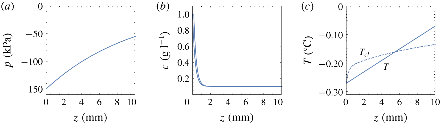
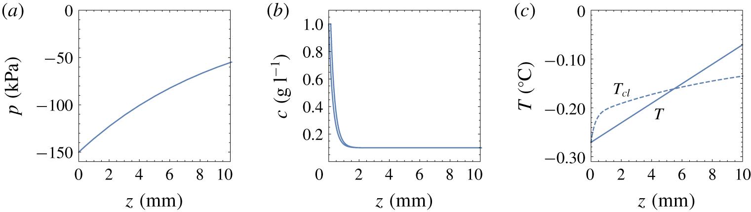
where  $p_{0}=p_{r}-\unicode[STIX]{x1D707}VH/k$. Equations (2.1), (2.6) and (2.7) are plotted on figure 2 for the case
 $V=1~\unicode[STIX]{x03BC}\text{m}~\text{s}^{-1}$,
 $c_{\infty }=0.1~\text{g}~\text{l}^{-1}$,
 $G_{T}=120~\text{K}~\text{m}^{-1}$,
 $P_{OB}=100~\text{kPa}$,
 $p_{r}=0$,
 $H=10~\text{cm}$, with physical and clay soil parameters
 $\unicode[STIX]{x1D707}=0.0015~\text{Pa}~\text{s}$,
 $C_{v}=10^{-8}~\text{m}^{2}~\text{s}^{-1}$,
 $k=10^{-16}~\text{m}^{2}$,
 $D=10^{-9}~\text{m}^{2}~\text{s}^{-1}$ and
 $k_{s}=0.1$.
Steady-state (a) pore pressure, (b) solute concentration and (c) temperature profiles in the soil below the ice lens in figure 1, calculated from (2.1), (2.6), (2.7) and (2.11). The dashed curve in (c) is the Clapeyron temperature (2.10). In the soil directly below the ice lens (between  $z=0$ and
 $z\approx 5~\text{mm}$), the temperature
 $T$ is less than the equilibrium freezing temperature
 $T_{Cl}$, and the soil is supercooled.
2.3 Ice lens temperature
The equilibrium freezing temperature  $T_{Cl}$ of the soil can be obtained from the generalized Clapeyron equation
 $$\begin{eqnarray}\frac{L_{f}(T_{Cl}-T_{m})}{T_{m}}=\unicode[STIX]{x1D708}_{w}(p-\unicode[STIX]{x03C0})-\unicode[STIX]{x1D708}_{i}p_{i},\end{eqnarray}$$
where  $T_{m}$ is the melting temperature of pure ice at atmospheric pressure,
 $\unicode[STIX]{x1D708}_{w/i}$ is the specific volume of water/ice,
 $L_{f}$ is the latent heat per unit mass of ice,
 $p_{i}$ is the ice pressure (relative to atmospheric pressure),
 $p$ is the pore fluid pressure (suction) and
 $\unicode[STIX]{x03C0}$ is the solute osmotic pressure (O’Neill Reference O’Neill1983; Acker, Elliott & McGann Reference Acker, Elliott and McGann2001; Peppin & Style Reference Peppin and Style2013). For dilute NaCl solutions
 $\unicode[STIX]{x03C0}=iRT_{m}C$, where
 $i\approx 2$ is the van’t Hoff coefficient,
 $R$ is the gas constant,
 $C=c/M_{s}$ is the molar concentration and
 $M_{s}=58.4~\text{g}~\text{mol}^{-1}$ is the NaCl molar mass. Neglecting the density difference between water and ice (
 $\unicode[STIX]{x1D708}_{i}=\unicode[STIX]{x1D708}_{w}=1/\unicode[STIX]{x1D70C}$), the Clapeyron equation (2.9) can be written as
 $$\begin{eqnarray}T_{Cl}=T_{m}-\frac{T_{m}}{\unicode[STIX]{x1D70C}L_{f}}(p_{i}-p)-mc,\end{eqnarray}$$
where  $\unicode[STIX]{x1D70C}$ is the density of water,
 $m=iK_{f}/M_{s}$ is the slope of the solute freezing temperature curve and
 $K_{f}=RT_{m}^{2}/(\unicode[STIX]{x1D70C}L_{f})=1.9~\text{Kl}~\text{mol}^{-1}$ is the molar cryoscopic constant. The other parameters used in (2.10) are
 $T_{m}=273.15~\text{K}$,
 $\unicode[STIX]{x1D70C}=1000~\text{kg}~\text{m}^{-3}$ and
 $L_{f}=3.3\times 10^{5}~\text{J}~\text{kg}^{-1}$ (table 1).
Assuming the ice lens pressure is equal to the overburden,  $p_{i}=P_{OB}$, the temperature
 $T_{0}$ at the ice lens–soil boundary
 $z=0$ can be obtained from (2.10) as
 $$\begin{eqnarray}T_{0}=T_{m}-\frac{T_{m}}{\unicode[STIX]{x1D70C}L_{f}}(P_{OB}-p_{0})-mc_{0},\end{eqnarray}$$
where  $p_{0}$ and
 $c_{0}$ are the pore pressure and solute concentration at
 $z=0$.
Physical parameters for water ice near  $0\,^{\circ }\text{C}$.

2.3.1 Constitutional and geometric supercooling
In solidification of aqueous solutions, constitutional supercooling of the solution adjacent to the ice interface occurs when  $\text{d}T_{L}/\text{d}z>\text{d}T/\text{d}z$, where
 $T_{L}=T_{m}-mc$ is the freezing temperature (liquidus) of the solution and
 $\text{d}T/\text{d}z=G_{T}$ is the temperature gradient (Worster Reference Worster1986; Davis Reference Davis2001). Constitutional supercooling typically leads to instabilities because perturbations of the interface move into supercooled regions and experience accelerated growth (Tiller et al. Reference Tiller, Jackson, Rutter and Chalmers1953; Davis Reference Davis2001).
Analogously, supercooling of the soil occurs when the gradient of the Clapeyron temperature is larger than the temperature gradient at the ice lens such that  $\text{d}T_{Cl}/\text{d}z>\text{d}T/\text{d}z$, or with (2.10),
 $$\begin{eqnarray}-m\frac{\text{d}c}{\text{d}z}+\frac{T_{m}}{\unicode[STIX]{x1D70C}L_{f}}\frac{\text{d}p}{\text{d}z}>\frac{\text{d}T}{\text{d}z}\quad (z=0).\end{eqnarray}$$
The first term on the left-hand side of (2.12) accounts for constitutional supercooling caused by solute diffusion, while the second term accounts for geometric (hydraulic) supercooling caused by viscous flow (Rempel Reference Rempel2008; Style et al. Reference Style, Peppin, Cocks and Wettlaufer2011; You et al. Reference You, Wang and Worster2018b). In terms of dimensionless parameters (2.12) can be written as
 $$\begin{eqnarray}{\mathcal{M}}_{c}+{\mathcal{M}}_{p}>1,\end{eqnarray}$$
where  ${\mathcal{M}}_{c}=-mG_{c}/G_{T}$ and
 ${\mathcal{M}}_{p}=T_{m}G_{p}/(\unicode[STIX]{x1D70C}L_{f}G_{T})$ are the solutal and hydraulic morphological numbers, respectively;
 $G_{c}=\text{d}c/\text{d}z|_{z=0}=-(c_{0}-c_{\infty })V/D$ and
 $G_{p}=\text{d}p/\text{d}z|_{z=0}=\unicode[STIX]{x1D707}V/k$ are the solute and pressure gradients at the ice lens interface. Figure 2(c) plots
 $T_{Cl}(z)$ and
 $T(z)$ for the pressure and solute profiles obtained in § 2.2, showing a supercooled region below the ice lens.
3 Linear stability analysis
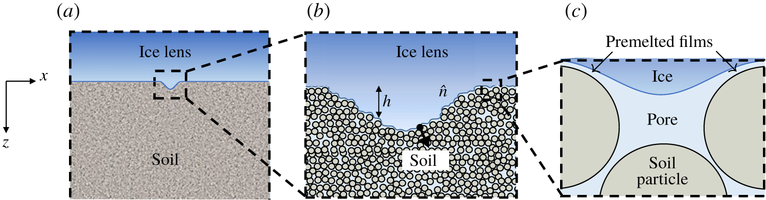
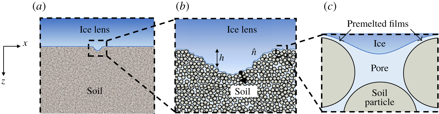
In linear stability analysis, the shape of the ice interface is perturbed, as in figure 3(a), and the governing equations are linearized about the planar steady-state solution. If the perturbations tend to diminish back to the planar state the ice lens is stable, while it is unstable if perturbations tend to grow. Assuming the linear temperature profile imposed by the boundary conditions is stable and not perturbed (frozen temperature approximation, Davis Reference Davis2001), the governing equations describing the evolution of the perturbed ice lens are
 $$\begin{eqnarray}\displaystyle & T=T_{0}+G_{T}z, & \displaystyle\end{eqnarray}$$
 $$\begin{eqnarray}\displaystyle & \displaystyle \frac{\unicode[STIX]{x2202}p}{\unicode[STIX]{x2202}t}-V\frac{\unicode[STIX]{x2202}p}{\unicode[STIX]{x2202}z}=C_{v}\unicode[STIX]{x1D6FB}^{2}p, & \displaystyle\end{eqnarray}$$
 $$\begin{eqnarray}\displaystyle & \displaystyle \frac{\unicode[STIX]{x2202}c}{\unicode[STIX]{x2202}t}-V\frac{\unicode[STIX]{x2202}c}{\unicode[STIX]{x2202}z}=D\unicode[STIX]{x1D6FB}^{2}c, & \displaystyle\end{eqnarray}$$
 $$\begin{eqnarray}\displaystyle V_{n}=\frac{k}{\unicode[STIX]{x1D707}}\unicode[STIX]{x1D735}p\boldsymbol{\cdot }\hat{n},\quad c_{h}(1-k_{s})V_{n}=-D\unicode[STIX]{x1D735}c\boldsymbol{\cdot }\hat{n}\quad (z=h),\end{eqnarray}$$
 $$\begin{eqnarray}T_{h}=T_{m}-mc_{h}-\frac{T_{m}}{\unicode[STIX]{x1D70C}_{l}L_{f}}(P_{OB}-p_{h})\quad (z=h),\end{eqnarray}$$
where  $h=h(x,t)$ is the height of the deformed interface and
 $$\begin{eqnarray}\hat{n}=\frac{(-h_{x},1)}{\sqrt{1+h_{x}^{2}}}\quad \text{and}\quad V_{n}=V\frac{(1+h_{t})}{\sqrt{1+h_{x}^{2}}}\end{eqnarray}$$
are, respectively, the unit normal  $\hat{n}$ to the ice lens surface and the ice velocity
 $V_{n}$ along the normal direction (Mullins & Sekerka Reference Mullins and Sekerka1964; Davis Reference Davis2001).
(a) Illustration of a macroscopic perturbation to the shape of the ice lens. If the perturbation continues to grow in size the ice lens is unstable; if all such perturbations melt back to the planar state the ice lens is stable. (b) The perturbed region is magnified, showing the height  $h(x)$ and the unit normal
 $\hat{n}$. (c) Further magnification shows the premelted films and the ice curvature on the pore scale.
As in § 2, latent heat and differing thermal conductivities are neglected and the temperature profile is assumed to be linear and stable. The frozen temperature approximation simplifies the analysis and allows the focus to be on the physical processes of diffusion and viscous flow that drive the ice lens instability. Accounting for latent heat effects leads to qualitatively similar results, with the thermal gradient  $G_{T}$ replaced by a weighted average
 $\bar{G}_{T}$ of the gradients in the frozen and unfrozen regions (Mullins & Sekerka Reference Mullins and Sekerka1964; Sekerka Reference Sekerka1968; Davis Reference Davis2001).
Before linearizing the equations it is convenient to write them in dimensionless form. The solutions (2.6) and (2.7) suggest the scalings
 $$\begin{eqnarray}(x^{\ast },z^{\ast })=\left(\frac{x}{\unicode[STIX]{x1D6FF}_{l}},\frac{z}{\unicode[STIX]{x1D6FF}_{l}}\right),\quad t^{\ast }=\frac{t}{\unicode[STIX]{x1D6FF}_{t}},\quad p^{\ast }=\frac{(p-p_{0})}{\unicode[STIX]{x1D6FF}_{l}G_{p}},\quad c^{\ast }=\frac{(c-c_{0})}{\unicode[STIX]{x1D6FF}_{l}G_{c}},\quad T^{\ast }=\frac{(T-T_{0})}{\unicode[STIX]{x1D6FF}_{l}G_{T}},\end{eqnarray}$$
where  $\unicode[STIX]{x1D6FF}_{l}=D/V$ and
 $\unicode[STIX]{x1D6FF}_{t}=D/V^{2}$ are length and time scales,
 $G_{p}=\unicode[STIX]{x1D707}V/k$ is the steady-state Darcy pressure gradient at
 $z=0$ and
 $G_{c}=-c_{0}V(1-k_{s})/D$ is the steady-state solute gradient at
 $z=0$. In dimensionless form the governing equations (3.1)–(3.3) become (upon dropping the stars)
 $$\begin{eqnarray}T=z,\quad p_{t}-p_{z}=\unicode[STIX]{x1D716}_{p}\unicode[STIX]{x1D6FB}^{2}p,\quad c_{t}-c_{z}=\unicode[STIX]{x1D6FB}^{2}c,\end{eqnarray}$$
where  $\unicode[STIX]{x1D716}_{p}=C_{v}/D$ is the ratio of the soil consolidation coefficient to the solute diffusivity. The boundary conditions (3.4) and (3.5) become
 $$\begin{eqnarray}\hat{V}_{n}=\unicode[STIX]{x1D735}p\boldsymbol{\cdot }\hat{n},\quad [c_{h}(1-k_{s})-1]\hat{V}_{n}=-\unicode[STIX]{x1D735}c\boldsymbol{\cdot }\hat{n}\quad (z=h),\end{eqnarray}$$
 $$\begin{eqnarray}T_{h}={\mathcal{M}}_{p}p_{h}+{\mathcal{M}}_{c}c_{h}\quad (z=h),\end{eqnarray}$$
where  $\hat{V}_{n}=V_{n}/V$ and the dimensionless numbers
 $$\begin{eqnarray}{\mathcal{M}}_{p}=\frac{T_{m}G_{p}}{\unicode[STIX]{x1D70C}L_{f}G_{T}}\quad \text{and}\quad {\mathcal{M}}_{c}=-\frac{mG_{c}}{G_{T}}\end{eqnarray}$$
are, respectively, the hydraulic and diffusive morphological numbers introduced in § 2.3.1. The steady base-state solutions (2.7) and (2.8) become, in terms of dimensionless quantities,
 $$\begin{eqnarray}\left[\begin{array}{@{}c@{}}c\\ p\\ h\end{array}\right]=\left[\begin{array}{@{}c@{}}\bar{c}\\ \bar{p}\\ \bar{h}\end{array}\right]=\left[\begin{array}{@{}c@{}}1-\text{e}^{-z}\\ \unicode[STIX]{x1D716}_{p}(1-\text{e}^{-z/\unicode[STIX]{x1D716}_{p}})\\ 0\end{array}\right].\end{eqnarray}$$
Let the base state be perturbed such that
 $$\begin{eqnarray}p=\bar{p}+p^{\prime },\quad c=\bar{c}+c^{\prime },\quad h=\bar{h}+h^{\prime },\end{eqnarray}$$
where the perturbations  $(p^{\prime },c^{\prime },h^{\prime })$ take the form of normal modes
 $$\begin{eqnarray}p^{\prime }=p_{1}(z)\text{e}^{\text{i}qx+\unicode[STIX]{x1D714}t},\quad c^{\prime }=c_{1}(z)\text{e}^{\text{i}qx+\unicode[STIX]{x1D714}t},\quad h^{\prime }=h_{1}(z)\text{e}^{\text{i}qx+\unicode[STIX]{x1D714}t}.\end{eqnarray}$$
Here  $q$ is the wavenumber and
 $\unicode[STIX]{x1D714}$ the growth rate of the perturbation (Mullins & Sekerka Reference Mullins and Sekerka1964; Davis Reference Davis2001). If
 $\unicode[STIX]{x1D714}<0$ for all wavenumbers
 $q$, the perturbations decay in time and the ice lens is stable, while if
 $\unicode[STIX]{x1D714}>0$ for any wavenumber the perturbation grows and the ice lens is unstable. In general the growth rate can also be a complex number, with the imaginary component describing oscillatory instabilities (Davis Reference Davis2001). An imaginary component to
 $\unicode[STIX]{x1D714}$ can appear, for example, if the segregation coefficient
 $k_{s}$ depends on the growth rate
 $V$ (Coriell & Sekerka Reference Coriell and Sekerka1983; Davis Reference Davis2001). In fact for lake ice
 $k_{s}$ does depend on
 $V$ (Weeks & Lofgren Reference Weeks and Lofgren1967), and experiments by Konrad & McCammon (Reference Konrad and McCammon1990) suggest the same is true for ice lenses. Here, for simplicity, the segregation coefficient is treated as an averaged constant so that
 $\unicode[STIX]{x1D714}$ is real (Sekerka Reference Sekerka1968; Wollkind & Segel Reference Wollkind and Segel1970) and the interface experiences only transverse wave instabilities.
Inserting (3.12) and (3.13) into (3.7), linearizing in the primed quantities and solving the resulting system of ordinary differential equations leads to the following expression for the growth rate  $\unicode[STIX]{x1D714}$ (appendix C)
 $$\begin{eqnarray}{\mathcal{M}}_{p}+{\mathcal{M}}_{c}=1+{\mathcal{M}}_{p}\frac{(\unicode[STIX]{x1D714}+\unicode[STIX]{x1D716}_{p}^{-1})}{r_{p}}+{\mathcal{M}}_{c}\frac{(\unicode[STIX]{x1D714}+k_{s})}{(k_{s}+r_{c}-1)},\end{eqnarray}$$
where
 $$\begin{eqnarray}r_{p}={\textstyle \frac{1}{2}}\unicode[STIX]{x1D716}_{p}^{-1}\left[1+\sqrt{1+4\unicode[STIX]{x1D716}_{p}(\unicode[STIX]{x1D714}+\unicode[STIX]{x1D716}_{p}q^{2})}\right]\quad \text{and}\quad r_{c}={\textstyle \frac{1}{2}}\left[1+\sqrt{1+4(\unicode[STIX]{x1D714}+q^{2})}\right].\end{eqnarray}$$
Equation (3.14) is a nonlinear equation for  $\unicode[STIX]{x1D714}$ that must in general be solved numerically. However, a simpler result can be obtained in the large wavenumber limit
 $q\gg 1$ (Mullins & Sekerka Reference Mullins and Sekerka1964; Davis Reference Davis2001). In this case
 $r_{p}\approx r_{c}\approx q$ and, assuming that
 $\unicode[STIX]{x1D716}_{p}^{-1}=D/C_{v}\ll 1$ and
 $k_{s}\ll 1$ (Bear Reference Bear1972; Davis Reference Davis2001), equation (3.14) becomes
 $$\begin{eqnarray}\unicode[STIX]{x1D714}\approx q(1-[{\mathcal{M}}_{p}+{\mathcal{M}}_{c}]^{-1}).\end{eqnarray}$$
Equation (3.15) shows that  $\unicode[STIX]{x1D714}$ is positive when
 ${\mathcal{M}}_{p}+{\mathcal{M}}_{c}>1$, and therefore the supercooling condition (2.13) leads to instability. The dimensional wavelength of the instability is
 $\unicode[STIX]{x1D706}=2\unicode[STIX]{x03C0}D/qV$ so that, for a salt diffusivity
 $D\sim 10^{-9}~\text{m}^{2}~\text{s}^{-1}$ and ice lens growth rate
 $V\sim 1~\unicode[STIX]{x03BC}\text{m}~\text{s}^{-1}$, the condition
 $q\gg 1$ implies
 $\unicode[STIX]{x1D706}\ll 1~\text{cm}$. Given the minimum observable size of segregated ice is of order the particle radius
 $R\sim 1~\unicode[STIX]{x03BC}\text{m}$, this suggests bounds on the initial wavelength of the form
 $1~\unicode[STIX]{x03BC}\text{m}\ll \unicode[STIX]{x1D706}\ll 1~\text{cm}$.
Setting  $\unicode[STIX]{x1D714}=0$ in (3.15) gives the marginal stability condition
 $$\begin{eqnarray}{\mathcal{M}}_{p}+{\mathcal{M}}_{c}=1.\end{eqnarray}$$
In terms of dimensional parameters the marginal stability condition (3.16) can be written as
 $$\begin{eqnarray}\frac{T_{m}\unicode[STIX]{x1D707}V}{G_{T}\unicode[STIX]{x1D70C}_{l}L_{f}k}+\frac{mc_{\infty }V(1-k_{s})}{Dk_{s}G_{T}}=1.\end{eqnarray}$$
The first term on the left-hand side of (3.17) accounts for geometric (hydraulic) supercooling, while the second term accounts for constitutional supercooling. This equation will be used in § 5 to study the stability of ice lenses in a clayey silt and a soil composed of glass microspheres. First, some implications of the instability are discussed in § 4.
4 Mushy layers in freezing porous media
4.1 Instability and mushy layer growth
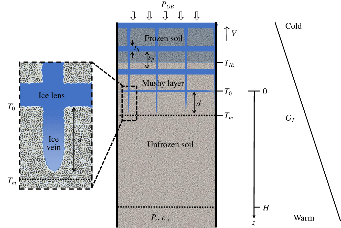
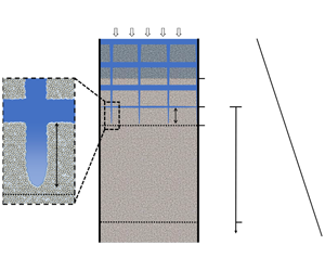
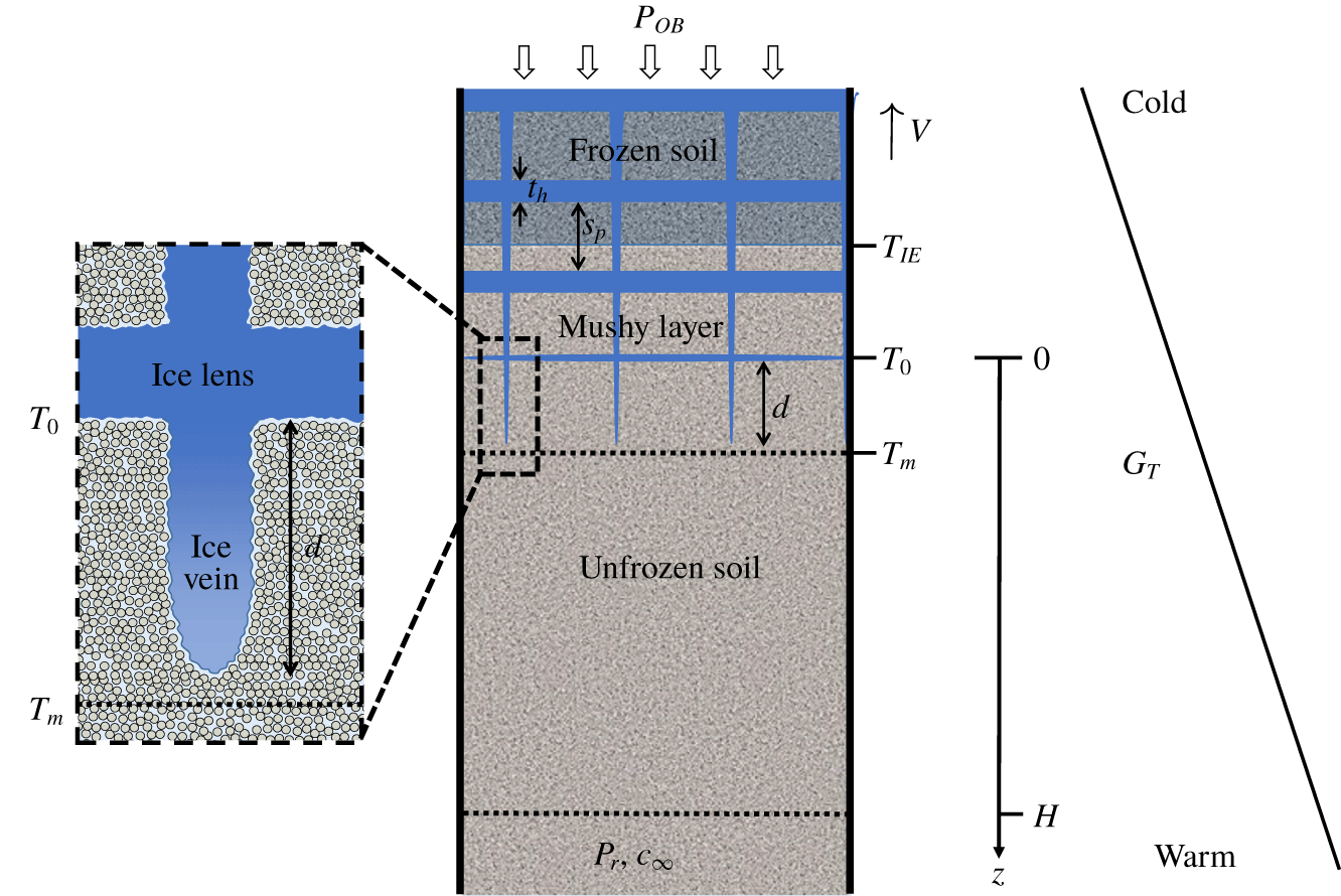
Morphological instability during the solidification of fluids leads to the formation of a mushy layer composed of vertical ice dendrites and interstitial fluid (Worster Reference Worster1986). The dendrites are a nonlinear manifestation of the planar instability and tend to form side branches in order to more efficiently remove the supercooling (Kurz & Fisher Reference Kurz and Fisher1998; Davis Reference Davis2001). Figure 4 illustrates a freezing soil in which a similar mushy layer has formed. The vertical ice veins in figure 4 are a nonlinear manifestation of the normal mode instability in § 3. In three dimensions ice veins tend to form a polygonal pattern in the soil cross-section (Taber Reference Taber1929; Mackay Reference Mackay1974; Chamberlain & Gow Reference Chamberlain and Gow1979; Arenson et al. Reference Arenson, Xia, Sego and Biggar2006; Arenson, Azmatch & Sego Reference Arenson, Azmatch and Sego2008; Wang et al. Reference Wang, Wang, Ma, Wen, Chen and Xu2018). Assuming the analogy with alloy solidification holds also for the vein spacing, the primary spacing  $\unicode[STIX]{x1D706}_{1}$ can be estimated as
 $$\begin{eqnarray}\unicode[STIX]{x1D706}_{1}=K_{1}C_{v}^{a}V^{-a}G_{T}^{-b},\end{eqnarray}$$
where  $a$,
 $b$ and
 $K_{1}$ are positive constants (Kurz & Fisher Reference Kurz and Fisher1998). Equation (4.1) indicates that the vein spacing decreases with the freezing speed
 $V$, and increases with the consolidation coefficient
 $C_{v}$, in qualitative agreement with the observations of Mackay (Reference Mackay1974, Reference Mackay1975) and Chamberlain & Gow (Reference Chamberlain and Gow1979). The horizontal ice lenses in figure 4 are assumed to nucleate as side branches from the vertical veins at the position of maximum supercooling (Style et al. Reference Style, Peppin, Cocks and Wettlaufer2011; You et al. Reference You, Wang, Wang, Wang, Lia and Lin2018a,Reference You, Wang and Worsterb). This ice lens nucleation mechanism is in contrast to secondary frost heave in which horizontal ice lenses form in the absence of ice veins via a regelation-induced fracture of the frozen fringe (Miller Reference Miller1978; Rempel, Wettlaufer & Worster Reference Rempel, Wettlaufer and Worster2004; Style et al. Reference Style, Peppin, Cocks and Wettlaufer2011).
Schematic diagram of a mushy layer in a freezing saline soil. The mushy layer is composed of vertical ice veins and horizontal ice lenses. The portion of the mushy layer between the warmest ice lens at temperature  $T_{0}$ and the freezing front near
 $T_{m}=0\,^{\circ }\text{C}$ is the (primary) frozen fringe, with thickness
 $d$.
 $T_{IE}$ is the temperature at which ice first enters the pore space. Here the system is experiencing primary frost heave (
 $T_{IE}<T_{0}$) and the soil surrounding the warmest ice lens is unfrozen. As in figure 1 there is a reservoir at
 $z=H$ containing pore fluid at pressure
 $p_{r}$ and solute concentration
 $c_{\infty }$. The system is moving at steady freezing speed
 $V$ within a fixed temperature gradient
 $G_{T}$ under an overburden pressure
 $P_{OB}$. This yields a uniform sequence of ice lenses, of average thickness
 $t_{h}$ and spacing
 $s_{p}$.
4.2 Primary and secondary frost heave
In figure 4  $T_{0}$ is the temperature of the warmest ice lens. The soil in between the ice lenses is unfrozen until the ice-entry temperature
 $T_{IE}$ is reached and ice begins to enter the pore space (Beskow Reference Beskow1935; Brown & Payne Reference Brown and Payne1990). In soils with a uniform pore size distribution the ice-entry temperature is given by the Gibbs–Thompson equation,
 $T_{IE}=T_{m}(1-2\unicode[STIX]{x1D6FE}/(R_{p}\unicode[STIX]{x1D70C}L_{f}))$, where
 $R_{p}$ is the pore size (Wettlaufer & Worster Reference Wettlaufer and Worster2006; Peppin & Style Reference Peppin and Style2013). Azmatch (Reference Azmatch2013) and Ginot et al. (Reference Ginot, Lenavetier, Dedovets and Deville2019) have shown that in soils with a broad size distribution or high salinity ice entry occurs over a finite range in temperature. In Miller’s classification scheme (Miller Reference Miller1972, Reference Miller1978) figure 4 is an example of (unstable) primary frost heave, because the warmest ice lens is forming in the absence of pore ice (
 $T_{0}>T_{IE}$). This is in contrast to secondary frost heave that occurs after ice has entered the pores (
 $T_{0}<T_{IE}$).
Current research is ongoing to distinguish between primary and secondary frost heave, with some works finding evidence for ice lens formation in soil containing pore ice (Loch & Miller Reference Loch and Miller1975; Konrad & Morgenstern Reference Konrad and Morgenstern1982; Walder & Hallet Reference Walder and Hallet1986; Anderson & Worster Reference Anderson and Worster2012, Reference Anderson and Worster2014; Schollick et al. Reference Schollick, Style, Curran, Wettlaufer, Dufresne, Warren, Velikov, Dullens and Aarts2016; You et al. Reference You, Wang and Worster2018b) and others finding ice lenses forming in soil regions that do not contain pore ice (Beskow Reference Beskow1935; Mackay Reference Mackay1975; Brown & Payne Reference Brown and Payne1990; Watanabe et al. Reference Watanabe, Mizoguchi, Ishizaki, Fukuda and Knutsson1997; Watanabe & Mizoguchi Reference Watanabe and Mizoguchi2000; You et al. Reference You, Wang, Wang, Wang, Lia and Lin2018a). It may be that both types of frost heave can occur in the same system depending on the freezing conditions (Schollick Reference Schollick2015; You et al. Reference You, Wang and Worster2018b). Microscale experiments capable of observing the pore contents during freezing, such as Raman spectroscopy (Watanabe & Mizoguchi Reference Watanabe and Mizoguchi2000), X-ray scattering (Spannuth et al. Reference Spannuth, Mochrie, Peppin and Wettlaufer2011) and confocal microscopy (Dedovets & Deville Reference Dedovets and Deville2018; Ginot et al. Reference Ginot, Lenavetier, Dedovets and Deville2019; Saint-Michel et al. Reference Saint-Michel, Georgelin, Deville and Pocheau2019) will play an important role in clarifying the situation.
4.3 The frozen fringe
In the context of secondary frost heave, Miller (Reference Miller1972, Reference Miller1978) defined the frozen fringe as the region between the warmest ice lens and the warmest extent of pore ice. Figure 4 suggests that a frozen fringe-like region can also be defined in the context of unstable primary frost heave as the region between the warmest ice lens and the warmest extent of segregated ice (tips of the ice veins). In the absence of solutes the ice veins extend very close to the  $0\,^{\circ }\text{C}$ isotherm, in which case the primary frozen fringe has thickness
 $d\approx (T_{m}-T_{0})/G_{T}$. In general, the frozen fringe can be defined as the region of soil between the warmest ice lens and the freezing front (warmest location of ice) (Konrad Reference Konrad1989b; Arenson et al. Reference Arenson, Azmatch and Sego2008).
4.3.1 Average permeability of the frozen fringe
In secondary frost heave the permeability  $k$ of the frozen fringe is reduced because of the presence of pore ice, which impedes the flow of water to the ice lens (Miller Reference Miller1978; Konrad & Morgenstern Reference Konrad and Morgenstern1981; Fowler & Krantz Reference Fowler and Krantz1994; Rempel et al. Reference Rempel, Wettlaufer and Worster2004). In the unstable primary frost heave occurring in figure 4, the permeability of the frozen-fringe region is also reduced because of consolidation of the soil between the ice veins, which reduces the pore size, and because of resistance to flow in premelted films at the ice lens–soil interface (Kuroda Reference Kuroda1987; Worster & Wettlaufer Reference Worster and Wettlaufer1999; Rempel Reference Rempel2008; Style & Peppin Reference Style and Peppin2012; You et al. Reference You, Wang and Worster2018b). Similarly to Konrad & Morgenstern (Reference Konrad and Morgenstern1980), the soil below the warmest ice lens can be modelled as a two-layer system with Darcy’s law written as
 $$\begin{eqnarray}V_{il}=\frac{p_{r}-p_{0}}{H\unicode[STIX]{x1D707}/k_{u}+d\unicode[STIX]{x1D707}/k},\end{eqnarray}$$
where  $V_{il}$ is the growth rate of the ice lens,
 $k_{u}$ is the permeability of the unfrozen soil and
 $k$ is the average permeability of the frozen fringe. In the case of no overburden pressure (
 $P_{OB}=p_{r}=0$) and zero salinity (
 $c_{0}=0$), the Clapeyron equation (2.11) can be combined with (4.2) to give
 $$\begin{eqnarray}V_{il}=\frac{(L_{f}/gT_{m})(T_{m}-T_{0})}{H/K_{u}+d/K},\end{eqnarray}$$
where  $K_{u}=\unicode[STIX]{x1D70C}gk_{u}/\unicode[STIX]{x1D707}$ is the hydraulic conductivity of the unfrozen soil,
 $K=\unicode[STIX]{x1D70C}gk/\unicode[STIX]{x1D707}$ is the hydraulic conductivity of the frozen fringe and
 $g$ is the acceleration due to gravity. By measuring the ice lens growth rate
 $V_{il}$, the ice lens temperature
 $T_{0}$, the temperature gradient
 $G_{T}$, the unfrozen soil height
 $H$ and hydraulic conductivity
 $K_{u}$, the frozen-fringe thickness can be calculated as
 $d=(T_{m}-T_{0})/G_{T}$, and (4.3) can be used to determine the frozen-fringe hydraulic conductivity
 $K$ (Konrad & Morgenstern Reference Konrad and Morgenstern1980). Style & Peppin (Reference Style and Peppin2012) determined the quantity
 $f=d/K$ as a function of temperature by modelling flow in the premelted films at the ice lens interface. While this leads to good results when applied to a system of uniform glass microparticles, parameters such as the premelted film viscosity in the expression for
 $f$ are not generally known as functions of overburden pressure and salinity. In the following a simpler approach is taken in which
 $K$ is treated as an averaged constant (Konrad & Morgenstern Reference Konrad and Morgenstern1981) or determined as a function of overburden via an empirical constitutive equation.
5 Applications
5.1 Devon silt
Devon silt is a clayey silt soil with a broad particle size distribution that is highly frost susceptible (Azmatch Reference Azmatch2013). Konrad & Morgenstern (Reference Konrad and Morgenstern1980, Reference Konrad and Morgenstern1981) measured the parameters in (4.3) for Devon silt at zero overburden and no salinity, and obtained a frozen-fringe thickness  $d\approx 1~\text{mm}$ and hydraulic conductivity
 $K\approx 10^{-11}~\text{m}~\text{s}^{-1}$. Konrad (Reference Konrad1990) also studied the effects of overburden pressure and salinity on ice lenses in Devon silt. The Clapeyron equation (2.11) shows that an overburden pressure
 $P_{OB}$ moves the ice lens temperature
 $T_{0}$ to lower values. This has the effect of reducing the premelted film thicknesses and further reducing the permeability. Black (Reference Black1990) reviewed various empirical equations that have been used to model the effect of an overburden pressure on the hydraulic conductivity of the frozen fringe. Here the Gardner equation is used in the form
 $$\begin{eqnarray}K=K_{0}\text{e}^{-\unicode[STIX]{x1D70E}^{\prime }/\unicode[STIX]{x1D70E}_{K}},\end{eqnarray}$$
where  $\unicode[STIX]{x1D70E}^{\prime }=P_{OB}-p_{0}$ is the effective stress on the soil matrix at
 $z=0$,
 $\unicode[STIX]{x1D70E}_{K}$ is a constant quantifying the effects of the overburden pressure on consolidation and flow in the premelted films and
 $K_{0}$ is the hydraulic conductivity of the frozen fringe at zero effective stress (Gilpin Reference Gilpin1982; Konrad & Morgenstern Reference Konrad and Morgenstern1984; Black Reference Black1990). An overburden pressure will also reduce the pore space available for solute diffusion, suggesting the diffusion coefficient be written as
 $$\begin{eqnarray}D=D_{0}\text{e}^{-\unicode[STIX]{x1D70E}^{\prime }/\unicode[STIX]{x1D70E}_{D}},\end{eqnarray}$$
where  $\unicode[STIX]{x1D70E}_{D}$ is a constant and
 $D_{0}$ is the diffusion coefficient of salt within the unstressed frozen fringe.
Azmatch (Reference Azmatch2013) measured the effective stress  $P_{OB}-p_{0}$ required for ice to enter the pores of Devon silt and found an ice-entry pressure of 175 kPa; the necessary pressure increased further when NaCl was added to the soil. The maximum overburden pressure in Konrad’s experiments was
 $P_{OB}=130~\text{kPa}$ and the average pore pressure (suction) at the ice lens was
 $p_{0}=-10~\text{kPa}$ (Konrad Reference Konrad1990), suggesting that the effective stress was not sufficient for ice to enter the pores below the ice lens, at least in the high salinity experiments. Konrad (Reference Konrad1990) noted that ‘layers of unfrozen soil’ may have been present between the ice lenses in his experiments because of the high salt concentrations. These results suggest that pore ice was not present in the frozen fringe of Konrad’s experiments, and that the system was undergoing unstable primary frost heave.
5.1.1 The segregation potential
Konrad & Morgenstern (Reference Konrad and Morgenstern1980, Reference Konrad and Morgenstern1981) introduced the segregation potential  $SP$, defined as
 $$\begin{eqnarray}SP=V_{il}/G_{T},\end{eqnarray}$$
where  $V_{il}$ and
 $G_{T}$ are measurements of the ice lens growth rate and temperature gradient at the onset of the formation of the final ice lens during transient freezing. For sufficiently small freezing rates
 $SP$ is a property of the soil, independent of the freezing parameters, and larger values of
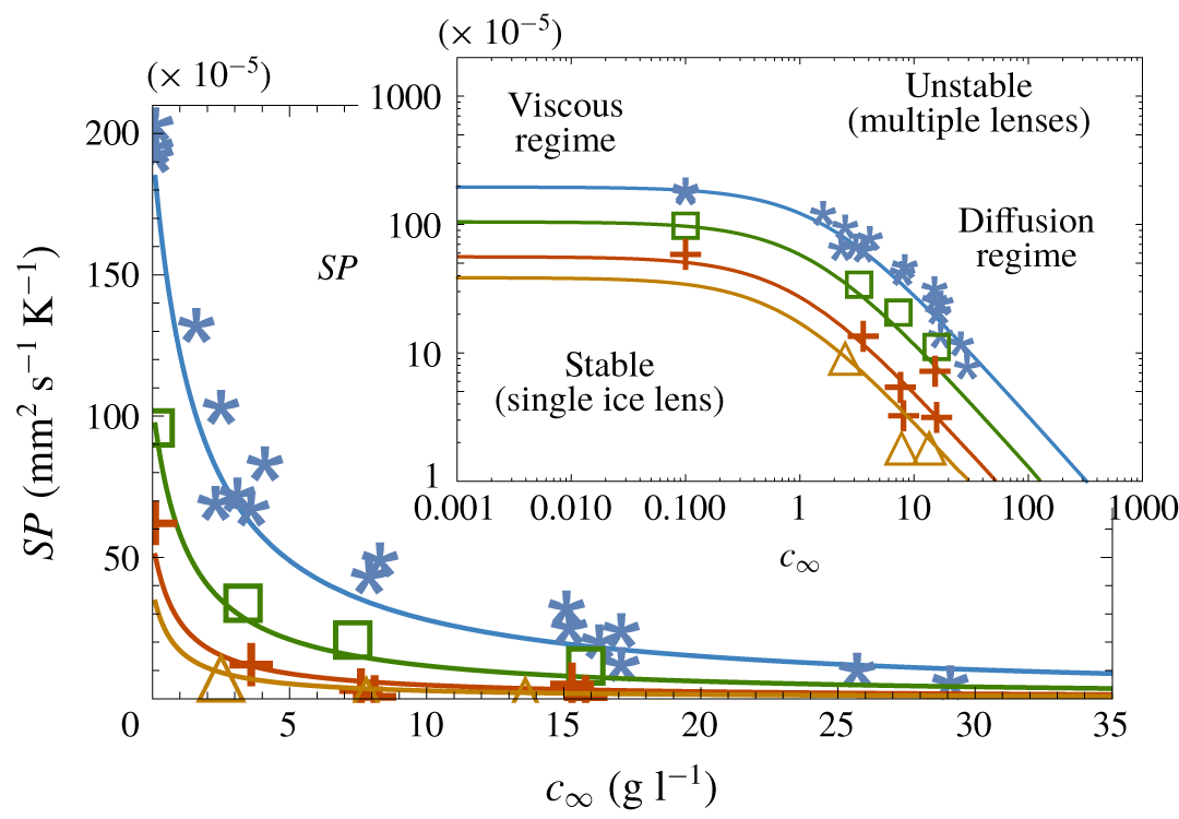
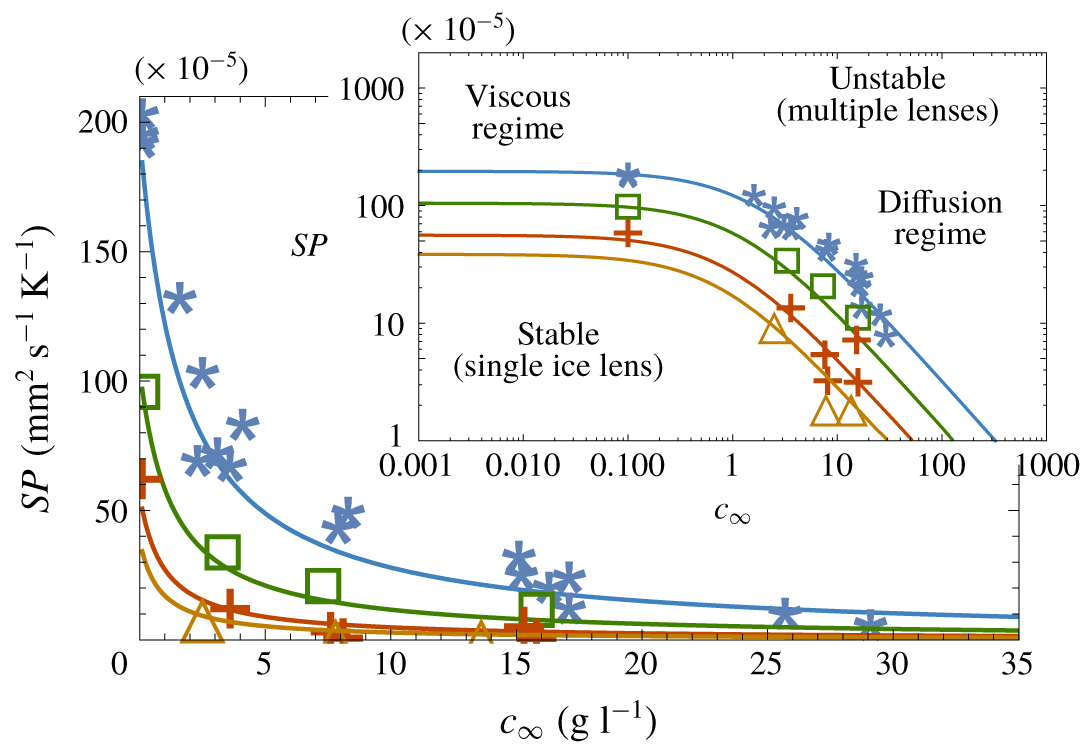
 $SP$ indicate a greater propensity of the soil to heave (Konrad & Morgenstern Reference Konrad and Morgenstern1981; Konrad Reference Konrad1987). Konrad (Reference Konrad1990) measured the segregation potential of Devon silt over a range of overburden pressures and salinities, shown in figure 5 as a regime diagram for
 $SP$ versus
 $c_{\infty }$. Assuming the onset of the final ice lens corresponds to a state of marginal stability such that
 $V_{il}\approx V$, the segregation potential can be obtained from (3.17) as
 $$\begin{eqnarray}SP=\left(\frac{T_{m}g}{L_{f}K}+\frac{mc_{\infty }(1-k_{s})}{Dk_{s}}\right)^{-1}.\end{eqnarray}$$
Plot of the segregation potential  $SP=V_{il}/G_{T}$ versus salinity
 $c_{\infty }$ for Devon silt; the data are from Konrad (Reference Konrad1990) at overburden pressures
 $P_{OB}=0~\text{kPa}$ (stars), 50 kPa (squares), 100 kPa (crosses) and 130 kPa (triangles) and average suction
 $p_{0}=-10~\text{kPa}$. The leftmost data points correspond to the background salinity in the soil used in the experiments, estimated by Konrad (Reference Konrad1990) as
 $c_{\infty }=0.1~\text{g}~\text{l}^{-1}$. The curves are from (5.4). The inset plots the data on a log scale, showing a viscous regime at low
 $c_{\infty }$ where
 $SP=L_{f}K/T_{m}g$, and a diffusion regime at high salinity where
 $SP=Dk_{s}/[mc_{\infty }(1-k_{s})]$.
5.1.2 Regime diagram
The curves in figure 5 show  $SP$ versus
 $c_{\infty }$ at several overburden pressures calculated from (5.4), using best-fit parameters
 $k_{s}=0.2$,
 $K_{0}=1.8\times 10^{-11}~\text{m}~\text{s}^{-1}$,
 $\unicode[STIX]{x1D70E}_{K}=80~\text{kPa}$,
 $D_{0}=10^{-9}~\text{m}^{2}~\text{s}^{-1}$ and
 $\unicode[STIX]{x1D70E}_{D}=55~\text{kPa}$ (other parameters such as
 $m$ and
 $L_{f}$ are as given in table 1). Below the curves the ice lens is predicted to grow stably (single ice lens), while above the curves it is unstable (mushy layer). There is a regime at low solute concentrations (
 $c_{\infty }<0.1~\text{g}~\text{l}^{-1}$) where the behaviour of the ice lens is independent of solute concentration, and the instability is caused by viscous flow through the soil layer and premelted films (geometric supercooling). In this regime the segregation potential (5.4) takes the limiting value
 $SP=L_{f}K/T_{m}g$. At high solute concentrations the instability is owing mainly to solute diffusion (constitutional supercooling); the first term on the right-hand side of (5.4) becomes negligible in this regime and
 $SP=Dk_{s}/[mc_{\infty }(1-k_{s})]$. As the background solute concentrations in soils are typically above
 $0.1~\text{g}~\text{l}^{-1}$ (Hivon & Sego Reference Hivon and Sego1993), these results suggest that frost heave often occurs in the diffusion regime, supporting the conclusions of Hallet (Reference Hallet1978) and Chamberlain (Reference Chamberlain1983) that solutes have significant effects on frost heave in periglacial soils.
The best-fit value for the hydraulic conductivity  $K_{0}$ of the frozen fringe is similar to that measured by Konrad & Morgenstern (Reference Konrad and Morgenstern1980) (
 $10^{-11}~\text{m}~\text{s}^{-1}$). The best-fit value for the NaCl segregation coefficient
 $k_{s}$ is similar to the measured value
 $k_{s}\approx 0.1$ for lake ice (Weeks & Lofgren Reference Weeks and Lofgren1967; Leppäranta Reference Leppäranta2015) but much larger than the equilibrium value (
 $k_{s}<10^{-3}$) for pure ice crystals (Gross, Gutjahr & Caylor Reference Gross, Gutjahr and Caylor1987). Konrad & McCammon (Reference Konrad and McCammon1990) also found that
 $k_{s}$ for Devon silt is larger than 0.1. Similarly Butler (Reference Butler2001) found, when freezing aqueous sucrose and polymer solutions, that a large segregation coefficient (
 $k_{s}>0.1$) was needed in the Mullins–Sekerka equation to accurately model the instability.
A potential explanation for the relatively large segregation coefficient is the presence of grain boundaries and defects in the ice. Weeks & Lofgren (Reference Weeks and Lofgren1967) show that lake ice is highly polycrystalline, in which case solute can be concentrated in between the grain boundaries (Thomson et al. Reference Thomson, Hansen-Goos, Wettlaufer and Wilen2013). Penner (Reference Penner1961) and Schollick (Reference Schollick2015) showed that ice lenses are also polycrystalline, and Wang et al. (Reference Wang, Wang, Ma, Wen, Chen and Xu2018) found that ice lenses contain significant defects that could also entrap salt. Furthermore, in soils such as Devon silt with a broad size distribution, salt could be transported in premelted films adjacent to the largest particles as they are engulfed by the ice during particle sorting (Corte Reference Corte1962; Körber Reference Körber1988). The ice–soil interface during lens growth is therefore a complex non-equilibrium system, with multiple mechanisms for solute entrapment, in contrast to the equilibrium ice–solution interface with a single ice grain used to obtain the much smaller equilibrium segregation coefficient (Gross et al. Reference Gross, Gutjahr and Caylor1987).
5.2 Glass powder
Watanabe et al. (Reference Watanabe, Muto and Mizoguchi2001), Watanabe (Reference Watanabe2002), Schollick (Reference Schollick2015) and Schollick et al. (Reference Schollick, Style, Curran, Wettlaufer, Dufresne, Warren, Velikov, Dullens and Aarts2016) performed a series of frost-heave experiments on a soil composed of approximately  $1~\unicode[STIX]{x03BC}\text{m}$ radius glass microparticles. Figure 4 is a schematic of their system, in which a Hele-Shaw cell containing the water-saturated powder is moved at speed
 $V$ through a temperature gradient
 $G_{T}$, yielding a sequence of equally spaced ice lenses. Watanabe et al. (Reference Watanabe, Muto and Mizoguchi2001) and Schollick (Reference Schollick2015) varied the salinity
 $c_{\infty }$ of the pore fluid and Watanabe (Reference Watanabe2002) and Schollick et al. (Reference Schollick, Style, Curran, Wettlaufer, Dufresne, Warren, Velikov, Dullens and Aarts2016) varied the freezing speed
 $V$, and the effects on the ice lens thicknesses
 $t_{h}$ and spacings
 $s_{p}$ were measured.
5.2.1 Steady-state mushy layer
The system in figure 4 can be modelled as a mushy layer containing segregated ice of volume fraction  $\unicode[STIX]{x1D6F7}$ (Worster Reference Worster1986; Peppin et al. Reference Peppin, Aussillous, Huppert and Worster2007). Developing a full mushy layer model is beyond the scope of the present work; however, some results can be obtained by writing the boundary conditions at the position of the warmest ice lens
 $z=0$ as
 $$\begin{eqnarray}V_{il}=\frac{k}{\unicode[STIX]{x1D707}}\frac{\text{d}p}{\text{d}z}\quad \text{and}\quad (c_{0}-c_{s})V=-D\frac{\text{d}c}{\text{d}z}\quad (z=0),\end{eqnarray}$$
where
 $$\begin{eqnarray}V_{il}=\unicode[STIX]{x1D6F7}V\quad \text{and}\quad c_{0}=\unicode[STIX]{x1D6F7}c_{s}/k_{s}+(1-\unicode[STIX]{x1D6F7})c_{s},\end{eqnarray}$$
are, respectively, the average growth speed  $V_{il}$ of the warmest ice lens and the average solute concentration
 $c_{0}$ at the ice lens. The first term in the expression for
 $c_{0}$ accounts for the solute rejected by the warmest ice lens, while the second term accounts for the solute trapped in between the ice lenses. When
 $\unicode[STIX]{x1D6F7}=1$ (single stable ice lens),
 $c_{0}=c_{\infty }/k_{s}$ as in § 2.2. At steady state
 $c_{s}=c_{\infty }$ is the average solute concentration in the mushy layer.
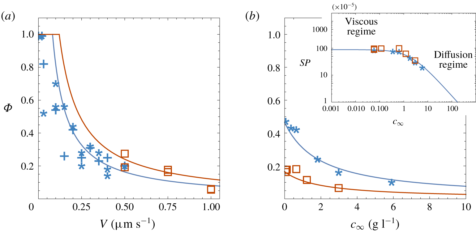
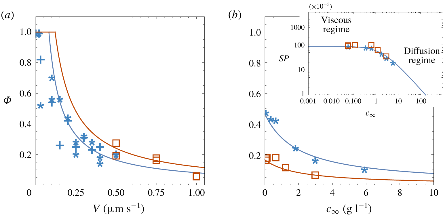
(a) Plot of segregated ice fraction  $\unicode[STIX]{x1D6F7}$ versus freezing rate
 $V$ for the case
 $c_{\infty }=0$. The data, from Watanabe (Reference Watanabe2002) (stars,
 $G_{T}=190~\text{K}~\text{m}^{-1}$) and Schollick et al. (Reference Schollick, Style, Curran, Wettlaufer, Dufresne, Warren, Velikov, Dullens and Aarts2016) (squares,
 $G_{T}=280~\text{K}~\text{m}^{-1}$), are from measurements of ice lens thicknesses
 $t_{h}$ and spacings
 $s_{p}$, with the segregated ice fraction determined as
 $\unicode[STIX]{x1D6F7}=t_{h}/(s_{p}+t_{h})$. Also shown are
 $\unicode[STIX]{x1D6F7}=V_{il}/V$ data (crosses) obtained from measurements of the ice lens growth rates
 $V_{il}$ (Watanabe Reference Watanabe2002). The curves are from (5.9). At low
 $V$ the ice lens is predicted to be stable (
 $\unicode[STIX]{x1D6F7}=1$). (b) Plot of
 $\unicode[STIX]{x1D6F7}$ versus the salinity
 $c_{\infty }$. The data are from ice lens thickness and spacing measurements of Watanabe et al. (Reference Watanabe, Muto and Mizoguchi2001) (stars,
 $V=0.4~\unicode[STIX]{x03BC}\text{m}~\text{s}^{-1}$,
 $G_{T}=210~\text{K}~\text{m}^{-1}$) and Schollick (Reference Schollick2015) (squares,
 $V=1.5~\unicode[STIX]{x03BC}\text{m}~\text{s}^{-1}$,
 $G_{T}=280~\text{K}~\text{m}^{-1}$). The leftmost data points correspond to the background salinity in the soil, estimated from figure 6 of Watanabe et al. (Reference Watanabe, Muto and Mizoguchi2001) as
 $c_{\infty }\approx 1~\text{mM}=0.06~\text{g}~\text{l}^{-1}$. The inset shows the segregation potential calculated as
 $SP=\unicode[STIX]{x1D6F7}V/G_{T}$. The curves are from (5.9) and (5.10).
Assuming that segregated ice forms to eliminate supercooling and return the system to local equilibrium (Worster Reference Worster1986), the temperature everywhere in the mushy layer is given by the Clapeyron equation (2.10). In the experiments the overburden and reservoir pressures were equal to atmospheric pressure so that  $P_{OB}=p_{i}=p_{r}=0$ and (2.10) becomes
 $$\begin{eqnarray}T_{Cl}=T_{m}+\frac{T_{m}}{\unicode[STIX]{x1D70C}L_{f}}p-mc.\end{eqnarray}$$
Following Worster (Reference Worster1986), the segregated ice fraction  $\unicode[STIX]{x1D6F7}$ in the mushy layer can be obtained by assuming marginal equilibrium in the mushy layer so that
 $$\begin{eqnarray}\frac{\text{d}T}{\text{d}z}=\frac{\text{d}T_{Cl}}{\text{d}z}\quad (z=0),\end{eqnarray}$$
 $$\begin{eqnarray}\unicode[STIX]{x1D6F7}=\frac{G_{T}}{V}\left(\frac{T_{m}g}{L_{f}K}+\frac{mc_{\infty }(1-k_{s})}{k_{s}D}\right)^{-1},\end{eqnarray}$$
where  $K=k\unicode[STIX]{x1D70C}g/\unicode[STIX]{x1D707}$ is the average hydraulic conductivity of the frozen fringe.
Figure 6 shows (a)  $\unicode[STIX]{x1D6F7}$ versus the freezing speed
 $V$ and (b)
 $\unicode[STIX]{x1D6F7}$ versus salinity
 $c_{\infty }$, calculated from (5.9), along with experimental data, with best-fit parameters
 $k_{s}=0.1$,
 $K=0.7\times 10^{-11}~\text{m}~\text{s}^{-1}$ and
 $D=10^{-9}~\text{m}^{2}~\text{s}^{-1}$. The best-fit hydraulic conductivity
 $K$ of the frozen fringe is similar to that for Devon silt (Konrad & Morgenstern Reference Konrad and Morgenstern1980), while the NaCl segregation coefficient
 $k_{s}$ is similar to that for lake ice (Leppäranta Reference Leppäranta2015). Also shown as the inset to figure 6(b) is the segregation potential estimated as
 $$\begin{eqnarray}SP=\frac{\unicode[STIX]{x1D6F7}V}{G_{T}}=\left(\frac{T_{m}g}{L_{f}K}+\frac{mc_{\infty }(1-k_{s})}{k_{s}D}\right)^{-1}.\end{eqnarray}$$
Similarly to the case of Devon silt, the  $SP$ diagram shows a viscous regime at low salinity and a diffusion regime at high salinity. The data of Watanabe et al. (Reference Watanabe, Muto and Mizoguchi2001) and Schollick (Reference Schollick2015), obtained using different freezing rates and temperature gradients, collapse onto a single
 $SP$ versus
 $c_{\infty }$ curve, supporting the conclusion of Konrad & Morgenstern (Reference Konrad and Morgenstern1981) that the segregation potential is a material property of the soil, independent of the freezing rate and temperature gradient. The magnitude of the segregation potential is less than the zero-overburden
 $SP$ data in figure 5, indicating that the glass powder is less frost susceptible than Devon silt.
6 Conclusions
A model of the growth of an ice lens during primary frost heave in a saline soil has been developed and a linear stability analysis undertaken, showing that a planar ice lens can become unstable because of supercooling. The characteristic equation for the marginal stability of the ice lens is related to the segregation potential of the soil. Segregation potential diagrams have been obtained for Devon silt and a glass powder medium, showing two distinct regimes: At low salinity the ice lens growth rate and stability are affected mainly by viscous flow in the soil and premelted films, while at high salinity they are controlled by salt diffusion. At unstable freezing rates a mushy layer, composed of a reticulate network of ice lenses and vertical ice veins, forms in order to remove the supercooling. A marginal equilibrium condition has been used to determine the segregated ice fraction in the mushy layer as a function of the salinity and freezing rate.
Acknowledgements
Discussions with and insights from D. G. A. L. Aarts, A. M. Anderson, P. Aussillous, S. Deville, J. A. W. Elliott, A. C. Fowler, P. Guba, M. G. Hennessey, H. E. Huppert, R. F. Katz, F. Lampl, J. R. Lister, C. B. Macdonald, A. Majumdar, J. A. Neufeld, D. Notz, M. D. Patterson, A. W. Rempel, S. M. Roper, G. C. Sander, J. M. H. Schollick, D. C. Sego, J. D. Sherwood, M. Spannuth, R. W. Style, E. S. Thomson, K. Watanabe, J. S. Wettlaufer, P. J. Williams, A. W. Woods and M. G. Worster are gratefully acknowledged, as are helpful comments from the referees. I thank Ontario Works and my family for financial support. All things were made by Him; and without Him was not any thing made that was made. John 1:3
Declaration of interests
The authors report no conflict of interest.
Appendix A
Assuming the porous medium is composed of inert incompressible particles and an incompressible fluid, conservation of mass can be written as
 $$\begin{eqnarray}\frac{\unicode[STIX]{x2202}\unicode[STIX]{x1D719}}{\unicode[STIX]{x2202}t}+\unicode[STIX]{x1D735}\boldsymbol{\cdot }\unicode[STIX]{x1D719}\boldsymbol{v}_{p}=0\quad \text{and}\quad \unicode[STIX]{x1D735}\boldsymbol{\cdot }\boldsymbol{v}=0,\end{eqnarray}$$
where  $\unicode[STIX]{x1D719}$ is the volume fraction of solids in a representative volume element,
 $1-\unicode[STIX]{x1D719}$ is the porosity,
 $\boldsymbol{v}_{p}$ is the average velocity of the porous matrix,
 $\boldsymbol{v}=\unicode[STIX]{x1D719}\boldsymbol{v}_{p}+(1-\unicode[STIX]{x1D719})\boldsymbol{v}_{f}$ is the volume average velocity of the mixture and
 $\boldsymbol{v}_{f}$ is the average fluid velocity (deGroot & Mazur Reference deGroot and Mazur1962; Bear Reference Bear1972). Using the identity
 $\unicode[STIX]{x1D735}\boldsymbol{\cdot }\unicode[STIX]{x1D719}\boldsymbol{v}=\unicode[STIX]{x1D719}\unicode[STIX]{x1D735}\boldsymbol{\cdot }\boldsymbol{v}+\boldsymbol{v}\boldsymbol{\cdot }\unicode[STIX]{x1D735}\unicode[STIX]{x1D719}$ (Bird, Stuart & Lightfoot Reference Bird, Stuart and Lightfoot2002) (A 1) can be combined to give
 $$\begin{eqnarray}\frac{\unicode[STIX]{x2202}\unicode[STIX]{x1D719}}{\unicode[STIX]{x2202}t}+\boldsymbol{v}\boldsymbol{\cdot }\unicode[STIX]{x1D735}\unicode[STIX]{x1D719}=\unicode[STIX]{x1D735}\boldsymbol{\cdot }\unicode[STIX]{x1D719}\boldsymbol{q},\end{eqnarray}$$
where  $\boldsymbol{q}=(\boldsymbol{v}-\boldsymbol{v}_{p})=(1-\unicode[STIX]{x1D719})(\boldsymbol{v}_{f}-\boldsymbol{v}_{p})$ is the volume velocity of the fluid relative to the porous matrix.
Assuming the pore pressure  $p=p(T,P,\unicode[STIX]{x1D719})$ is independent of temperature
 $T$ and mixture pressure
 $P$, differentiating
 $p$ gives
 $$\begin{eqnarray}\text{d}p=\left(\frac{\unicode[STIX]{x2202}p}{\unicode[STIX]{x2202}\unicode[STIX]{x1D719}}\right)_{T,P}\,\text{d}\unicode[STIX]{x1D719}=-\frac{1}{m_{v}}\,\text{d}\unicode[STIX]{x1D719},\end{eqnarray}$$
where  $m_{v}=(\unicode[STIX]{x2202}\unicode[STIX]{x1D719}/\unicode[STIX]{x2202}\unicode[STIX]{x1D70E}^{\prime })_{T,P}$ is the soil volume compressibility and
 $\unicode[STIX]{x1D70E}^{\prime }\equiv P-p$ is the effective stress on the soil matrix. Darcy’s law can be written in the form
 $$\begin{eqnarray}\boldsymbol{q}=-\frac{k}{\unicode[STIX]{x1D707}}\unicode[STIX]{x1D735}p,\end{eqnarray}$$
where  $k$ is the permeability and
 $\unicode[STIX]{x1D707}$ the fluid viscosity (Bear Reference Bear1972; Bear & Corapcioglu Reference Bear and Corapcioglu1981). Combining (A 3) and (A 4) with (A 2) and assuming
 $\unicode[STIX]{x1D719}k/\unicode[STIX]{x1D707}$ is constant gives the pressure diffusion equation
 $$\begin{eqnarray}\frac{\unicode[STIX]{x2202}p}{\unicode[STIX]{x2202}t}+\boldsymbol{v}\boldsymbol{\cdot }\unicode[STIX]{x1D735}p=C_{v}\unicode[STIX]{x1D735}\boldsymbol{\cdot }\unicode[STIX]{x1D735}p,\end{eqnarray}$$
where  $C_{v}=\unicode[STIX]{x1D719}k/(\unicode[STIX]{x1D707}m_{v})$ is the consolidation coefficient. Finally, considering a one-dimensional system with
 $\boldsymbol{v}=-V\hat{z}$ gives (2.2).
Appendix B
At steady state  $\unicode[STIX]{x2202}p/\unicode[STIX]{x2202}t=\unicode[STIX]{x2202}c/\unicode[STIX]{x2202}t=0$ and (2.2) and (2.3) become
 $$\begin{eqnarray}C_{v}\frac{\text{d}^{2}p}{\text{d}z^{2}}+V\frac{\text{d}p}{\text{d}z}=0,\quad D\frac{\text{d}^{2}c}{\text{d}z^{2}}+V\frac{\text{d}c}{\text{d}z}=0,\end{eqnarray}$$
subject to the boundary conditions
 $$\begin{eqnarray}V=\frac{k}{\unicode[STIX]{x1D707}}\frac{\text{d}p}{\text{d}z},\quad (c_{0}-c_{s})V=-D\frac{\text{d}c}{\text{d}z}\quad (z=0),\end{eqnarray}$$
and
 $$\begin{eqnarray}p=p_{r}\quad (z=H)\quad \text{and}\quad c\rightarrow c_{\infty }\quad (z\rightarrow \infty ),\end{eqnarray}$$
where  $c_{s}=c_{\infty }$ and
 $c_{0}=c_{\infty }/k_{s}$. The general solutions to (B 1) are of the form
 $$\begin{eqnarray}p=A_{p}+B_{p}\text{e}^{r_{p}z}\quad \text{and}\quad c=A_{c}+B_{c}\text{e}^{r_{c}z},\end{eqnarray}$$
where  $A_{p,c},B_{p,c},r_{p,c}$ are constants. Inserting (B 4) into (B 1) gives
 $r_{p}=-V/C_{v}$ and
 $r_{c}=-V/D$; inserting (B 4) into (B 2) gives
 $B_{p}=-C_{v}\unicode[STIX]{x1D707}/k$ and
 $B_{c}=c_{0}-c_{\infty }$; equations (B 3) then require
 $A_{p}=p_{r}+(C_{v}\unicode[STIX]{x1D707}/k)\text{e}^{-VH/C_{v}}$ and
 $A_{c}=c_{\infty }$, giving (2.6) and (2.7).
Appendix C
Inserting (3.12) into (3.7) and linearizing in the primed quantities gives, bearing in mind that for the steady base state  $\bar{c}_{z}+\unicode[STIX]{x1D6FB}^{2}\bar{c}=0$ and
 $\bar{p}_{z}+\unicode[STIX]{x1D716}_{p}\unicode[STIX]{x1D6FB}^{2}\bar{p}=0$,
 $$\begin{eqnarray}\displaystyle & p_{t}^{\prime }-p_{z}^{\prime }=\unicode[STIX]{x1D716}_{p}\unicode[STIX]{x1D6FB}^{2}p^{\prime }, & \displaystyle\end{eqnarray}$$
 $$\begin{eqnarray}\displaystyle & c_{t}^{\prime }-c_{z}^{\prime }=\unicode[STIX]{x1D6FB}^{2}c^{\prime }. & \displaystyle\end{eqnarray}$$
Inserting  $p^{\prime }$ and
 $c^{\prime }$ from (3.13) into (C 1) and (C 2), and neglecting terms nonlinear in the perturbations, leads to the ordinary differential equations
 $$\begin{eqnarray}\displaystyle & \displaystyle \unicode[STIX]{x1D716}_{p}\frac{\text{d}^{2}p_{1}}{\text{d}z^{2}}+\frac{\text{d}p_{1}}{\text{d}z}-(\unicode[STIX]{x1D714}+\unicode[STIX]{x1D716}_{p}q^{2})p_{1}=0\quad (z>0), & \displaystyle\end{eqnarray}$$
 $$\begin{eqnarray}\displaystyle & \displaystyle \frac{\text{d}^{2}c_{1}}{\text{d}z^{2}}+\frac{\text{d}c_{1}}{\text{d}z}-(\unicode[STIX]{x1D714}+q^{2})c_{1}=0\quad (z>0). & \displaystyle\end{eqnarray}$$
Assuming the perturbations decay far from the ice lens, the far-field boundary conditions are
 $$\begin{eqnarray}p_{1}\rightarrow 0,\quad c_{1}\rightarrow 0\quad (z\rightarrow \infty ).\end{eqnarray}$$
The solutions to (C 3) and (C 4) subject to (C 5) are
 $$\begin{eqnarray}p_{1}=A\text{e}^{-r_{p}z}\quad \text{and}\quad c_{1}=B\text{e}^{-r_{c}z},\end{eqnarray}$$
where  $A$ and
 $B$ are constants,
 $$\begin{eqnarray}r_{p}={\textstyle \frac{1}{2}}\unicode[STIX]{x1D716}_{p}^{-1}\left[1+\sqrt{1+4\unicode[STIX]{x1D716}_{p}(\unicode[STIX]{x1D714}+\unicode[STIX]{x1D716}_{p}q^{2})}\right]\quad \text{and}\quad r_{c}={\textstyle \frac{1}{2}}\left[1+\sqrt{1+4(\unicode[STIX]{x1D714}+q^{2})}\right].\end{eqnarray}$$
The boundary conditions (3.8) at the perturbed ice interface  $z=h$ can be expanded via Taylor series about
 $z=0$ (Davis Reference Davis2001). To first order and neglecting terms nonlinear in the primed quantities, bearing in mind that
 $\bar{c}(0)=0$ and
 $\bar{c}_{z}(0)=1$,
 $$\begin{eqnarray}c_{h}=c(h)\approx c(0)+hc_{z}(0)=[\bar{c}(0)+c^{\prime }(0)]+h[\bar{c}_{z}(0)+c_{z}^{\prime }(0)]\approx c^{\prime }(0)+h^{\prime }.\end{eqnarray}$$
Similarly,
 $$\begin{eqnarray}c_{z}(h)\approx 1-h^{\prime }+c_{z}^{\prime }(0),\quad p_{h}=p(h)\approx h^{\prime }+p^{\prime }(0)\quad \text{and}\quad p_{z}(h)\approx 1-h^{\prime }\unicode[STIX]{x1D716}_{p}^{-1}+p_{z}^{\prime }(0).\end{eqnarray}$$
Inserting these expansions into (3.8) gives, upon neglecting nonlinear terms and using the linearized quantities  $\hat{n}\approx (-h_{x}^{\prime },1)$ and
 $V_{n}\approx V(1+h_{t}^{\prime })$,
 $$\begin{eqnarray}p_{z}^{\prime }=h_{t}^{\prime }+h^{\prime }\unicode[STIX]{x1D716}_{p}^{-1}\quad \text{and}\quad c_{z}^{\prime }=h_{t}^{\prime }+h^{\prime }k_{s}-c^{\prime }(1-k_{s})\quad (z=0).\end{eqnarray}$$
Combining equations (3.7a) and (3.9) at  $z=h$ and expanding about
 $z=0$ gives
 $$\begin{eqnarray}h^{\prime }={\mathcal{M}}_{p}(h^{\prime }+p^{\prime })+{\mathcal{M}}_{c}(h^{\prime }+c^{\prime })\quad (z=0).\end{eqnarray}$$
With (3.13) the boundary conditions (C 7) become
 $$\begin{eqnarray}\frac{\text{d}p_{1}}{\text{d}z}=(\unicode[STIX]{x1D716}_{p}^{-1}+\unicode[STIX]{x1D714})h_{1},\quad \frac{\text{d}c_{1}}{\text{d}z}=-c_{1}(1-k_{s})+(k_{s}+\unicode[STIX]{x1D714})h_{1}\quad (z=0),\end{eqnarray}$$
and (C 8) gives
 $$\begin{eqnarray}h_{1}=\frac{{\mathcal{M}}_{p}p_{1}+{\mathcal{M}}_{c}c_{1}}{1-({\mathcal{M}}_{p}+{\mathcal{M}}_{c})}.\end{eqnarray}$$
Eliminating  $h_{1}$ between (C 9) and (C 10), and inserting the solutions (C 6) into the result, leads to the characteristic equation (3.14).