1. Introduction
Swirling flows with a free surface can undergo remarkable symmetry-breaking transitions, where an originally rotationally symmetric surface spontaneously deforms into a rotating polygonal state (Vatistas Reference Vatistas1990; Jansson et al.
Reference Jansson, Haspang, Jensen, Hersen and Bohr2006; Suzuki, Iima & Hayase Reference Suzuki, Iima and Hayase2006). In the laboratory experiments, a cylindrical container is filled to a certain height with liquid (usually water) and the bottom plate is rotated while the cylinder remains at rest (Vatistas Reference Vatistas1990; Vatistas, Wang & Lin Reference Vatistas, Wang and Lin1992; Jansson et al.
Reference Jansson, Haspang, Jensen, Hersen and Bohr2006; Suzuki et al.
Reference Suzuki, Iima and Hayase2006; Vatistas, Abderrahmane & Kamran Siddiqui Reference Vatistas, Abderrahmane and Kamran Siddiqui2008; Tasaka & Iima Reference Tasaka and Iima2009; Bergmann et al.
Reference Bergmann, Tophøj, Homan, Hersen, Andersen and Bohr2011, Reference Bergmann, Tophøj, Homan, Hersen, Andersen and Bohr2012; Mandour et al.
Reference Mandour, Fayed, Abderrahmane, Ng, Kadem and Vatistas2012; Abderrahmane et al.
Reference Abderrahmane, Fayed, Ng and Vatistas2013). Recently, Tophøj et al. (Reference Tophøj, Mougel, Bohr and Fabre2013) have observed that the rotating polygon instability also occurs more generally for a fluid with very low friction, e.g. when liquid nitrogen undergoing film boiling is set into rotation in a stationary container and slowly spins down. These authors present a theory of the instability based on potential flow, assuming that the basis flow is close to a simple line vortex. Since the azimuthal velocity in a line vortex flow diverges like
 $1/r$
, where
 $r$
is the distance to the rotational axis, this theory is limited to the ‘dry’ states in which a central region of the bottom plate is free of fluid. In this case, the instability has been explained as a resonance between gravity waves (near the cylinder wall) and centrifugal waves (the ‘polygons’ near the centre). A theory of the fully developed states has been presented by Amaouche, Abderrahmane & Vatistas (Reference Amaouche, Abderrahmane and Vatistas2013), where the polygonal surface deformations are described as travelling cnoidal waves. Poncet & Chauve (Reference Poncet and Chauve2007) show images that seem very close to those presented in the above studies. However, they study a very different situation, where the Reynolds number is so low that there is no appreciable surface deformation. The ‘polygons’ are thus formed by flow visualisation, and contrary to the surface polygons studied in the present work, the Reynolds number is an important parameter.
Clearly, the line vortex flow can at best be an approximation, neglecting both secondary radial flow and the considerable turbulence observed. It is therefore important to vary the basis state and to see, which basis states would actually be unstable to polygon formation. As an example, the famous Newton’s bucket flow, where the entire cylinder and fluid volume is in rigid-body rotation, and which was used by Newton to contrast inertial (non-rotating) reference frames with accelerated (rotating) ones, is not expected to give rise to any instabilities (Fabre & Mougel Reference Fabre and Mougel2014).
In order to explore the symmetry-breaking instability further, we have made an experimental set-up where we can independently control the rotation rates of the bottom plate
 $f_{b}$
and the cylinder
 $f_{c}$
, and thereby vary the overall rotation rate and shear rate independently. Thus, we can move from a state (
 $f_{c}=f_{b}$
, Newton’s bucket) where the fluid is at rest in the rotating frame and receives a maximal rotation with no shear, to a state (
 $f_{c}=-f_{b}$
) where the rotation rate of the fluid is minimal and the shear rate is maximal, which is reflected by an almost flat surface and strong turbulence.
In this paper we present the first results from measurements with this set-up, in particular highlighting the region of the phase diagram, where instability can occur and the types of such instabilities. We find that instability occurs roughly in a region along a line
 $3f_{c}+f_{b}=\text{const.}$
of the
 $(\,f_{b},f_{c})$
-plane, with, predominantly, counter-rotation of plate and cylinder (negative
 $f_{c}$
). Furthermore, we find that two distinct bands of polygons appear at sufficiently large
 $f_{b}$
. We shall first explain the set-up and then describe the phase diagram, first only rotating the bottom plate and second when we combine bottom plate and cylinder rotation. We shall compare our results when we only rotate the bottom plate with the results of Jansson et al. (Reference Jansson, Haspang, Jensen, Hersen and Bohr2006), and we show that although the overall features are the same, they differ in detail. To investigate possible reasons for these differences, we have measured the rotation rate of the polygons, in particular to rule out the possibility of phase locking between the bottom plate and the figure, which might have caused such differences. Finally, we show that there is a considerable multistability and excitability of the polygonal states, which might explain why small differences in set-up can cause changes in the phase diagram.
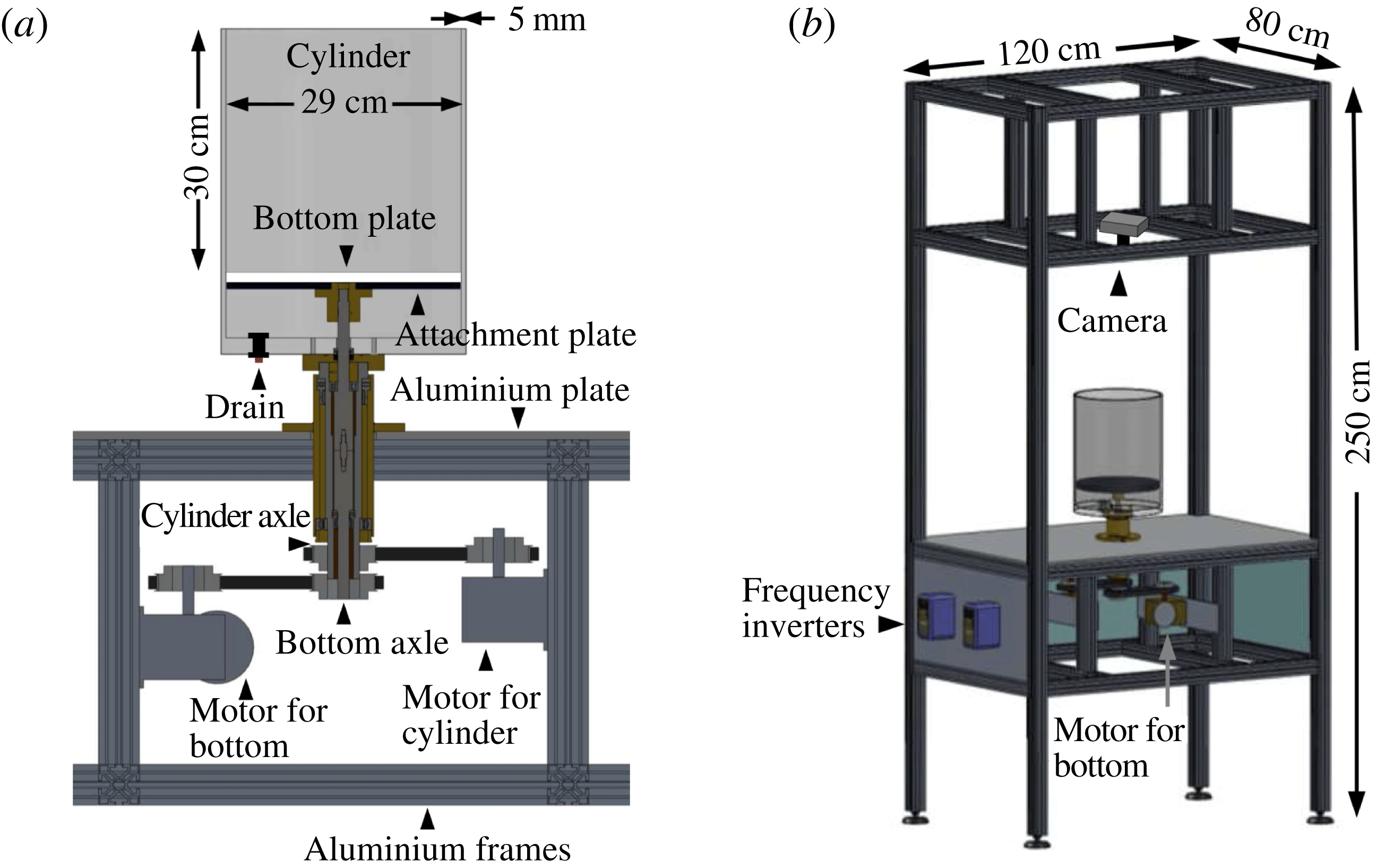
The experimental set-up. (a) The Plexiglas cylinder and the bottom plate can rotate independently. (b) The complete set-up with the embedding of the cylinder in a large and heavy aluminium construction which helps to stabilise the dynamics.

2. Experimental set-up
Our experimental set-up is shown in figure 1. A Plexiglas cylinder with inner diameter 29 cm has a Plexiglas bottom plate mounted 30 cm from the top rim such that both the cylinder and the plate can rotate independently, controlled by separate motors. The ‘bottom’ plate is actually not placed at the bottom of the cylindrical container, but 10 cm above to let it rotate freely. The horizontal gap between the bottom plate and the cylinder is less than 1 mm and thus the fluid below the bottom plate does not play a role. Both the cylinder and the bottom plate can rotate with frequencies between 0.4 and 6.9 Hz both clockwise and counter-clockwise. The entire construction is large compared with the cylinder. The rack has dimensions of
 $120\ \text{cm}\times 80\ \text{cm}\times 250\ \text{cm}$
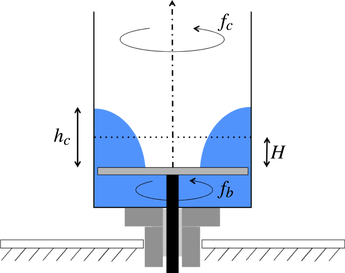
, is made of aluminium, and weighs 140 kg. The vertical axis of rotation and the horizontal bottom plate are accurately set up, but the cylinder available to us has a slight skewness, introducing a wobbling of approximately 0.4°. To secure stability of the bottom plate and smoothness of its upper surface, we mounted it with screws from below to an attachment plate of the same size. We used two different bottom plates, one in black and one in white. The best pictures and visualisations are made with the white plate and a few drops of red dye to enhance the contrast. Figure 2 shows the three control parameters that we shall vary in the following, namely the rotational frequencies of the bottom plate,
 $f_{b}$
, and of the cylinder,
 $f_{c}$
, and the filling height of the water,
 $H$
, i.e. the water height when both the bottom plate and the cylinder are at rest. The experiment is illuminated by a LED strip encircling the cylinder approximately 5 cm above the upper surface of the bottom plate.
Sketch of cylinder and bottom plate with parameters.

3. Polygons with rotating bottom and stationary cylinder
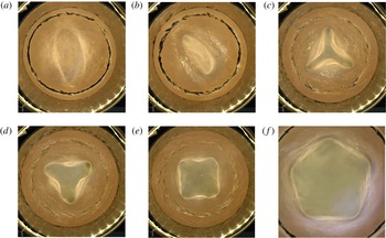
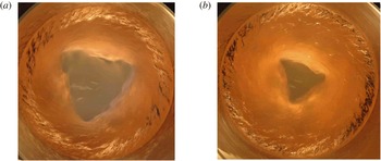
We first look at the case where the cylinder is stationary and only the bottom plate rotates. Typical polygonal states are shown in figure 3. This case has been studied earlier and we shall compare our results in § 5 with Vatistas (Reference Vatistas1990), Vatistas et al. (Reference Vatistas, Wang and Lin1992) and Jansson et al. (Reference Jansson, Haspang, Jensen, Hersen and Bohr2006). To obtain a phase diagram, we vary the filling height of the water
 $H$
from 30 to 80 mm with steps of 10 mm. For each water level the rotational frequency of the bottom plate
 $f_{b}$
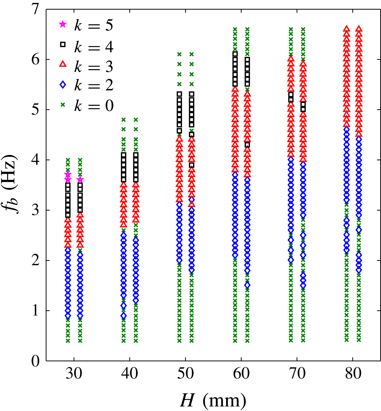
is increased from 0.4 Hz with steps of 0.1 Hz up to a value where no more polygons are seen and the states regain the rotational symmetry. Every time the frequency is increased, we wait 1 min to let the flow equilibrate to what seems to be the stationary rotating state. The polygonal states are characterised by noting the number of corners of the stable states. To check for possible multistability, a large perturbation of the flow is made by hand to reset the flow, and the number of corners in the resulting state which the flow now finds is noted. The flow is perturbed between two and five times. The resulting phase diagram is shown in figure 4. The number of corners of the polygonal shape is denoted
 $k$
. The case
 $k=0$
denotes either a circular shape, or that no definite shape could be determined. Each data point consist of two symbols. If these are the same, it means that the state was stable and it kept its polygonal form after the perturbations. If they are different, it means that both states can occur. The left state is the one that appears first and the right one is the most probable alternative state. We have not distinguished between ‘wet’ polygons, where the bottom plate is entirely covered by water (figure 3
a) and ‘dry’ cases, with a dry central region (figure 3
b,c).
Snapshots of the polygons with stationary cylinder (
 $f_{c}=0\ \text{Hz}$
) at
 $H=60\ \text{mm}$
for (a)–(e) and at
 $H=30\ \text{mm}$
for ( f): (a)
 $f_{b}=3.0\ \text{Hz}$
, ellipse (
 $k=2$
); (b)
 $f_{b}=3.4\ \text{Hz}$
, ellipse (
 $k=2$
); (c)
 $f_{b}=4.6\ \text{Hz}$
, triangle (
 $k=3$
); (d)
 $f_{b}=5.0\ \text{Hz}$
, triangle (
 $k=3$
); (e)
 $f_{b}=5.8\ \text{Hz}$
, square (
 $k=4$
); and ( f)
 $f_{b}=3.6\ \text{Hz}$
, pentagon (
 $k=5$
). The bright circle around the cylinder is the LED strip used for illumination. The dark circle, especially apparent in (a), (b) and ( f) is the reflection of the rim of the black attachment plate (figure 1
a) in the cylinder.

Phase diagram in the experiment with rotating bottom plate and stationary cylinder wall. The diagram is spanned by the filling height,
 $H$
, and the rotational frequency of the bottom plate,
 $f_{b}$
. The symmetries of the states are indicated by the symbols in the legend.

For frequencies higher than 1 Hz, polygonal shapes occur (figure 4). Increasing the frequency, they first become elliptical, next triangular, then squares and finally in some cases pentagonal, before they become unstable, i.e. non-stationary or circular again. The order of polygons for increasing frequencies are consistent with both Vatistas (Reference Vatistas1990) and Jansson et al. (Reference Jansson, Haspang, Jensen, Hersen and Bohr2006). The thresholds for going from one polygon to the next slightly increase with filling height
 $H$
. Thus, the threshold for triangles increases by around 0.5 Hz for each 10 mm water added, and for the threshold of squares it is around 0.8 Hz for each 10 mm water added. The border between different states consists of a transition band with a considerable hysteresis and multistability, to which we shall return in § 6. In particular, going from circles to ellipses, there is a large area with unstable states for
 $H$
between 70 and 80 mm, i.e. states that never become fully stationary. Similarly, Vatistas (Reference Vatistas1990) found that there are transition bands between the different stable polygons, where the shape is a distorted, unstable version of the ‘upper’ polygonal shape.
Surprisingly, we find a thin bistable band, where squares are also stable, inside the region of triangles for
 $H$
between 50 and 70 mm. For
 $H=50\ \text{mm}$
and
 $H=60\ \text{mm}$
the triangles were dominating, whereas they were equally likely for
 $H=70\ \text{mm}$
. It also looks as if a region of squares is missing after the triangles for
 $H=70\ \text{mm}$
but they do not occur in the experiments despite many attempts and long stabilisation times. We only find pentagons for
 $H=30\ \text{mm}$
, despite many experimental attempts in the areas just above the squares, where we expected to find them. The pentagons found are stable, but in some realisations it took more than 5 min before they stabilised into a regular form. So we cannot exclude that they can be found also in other places, but simply did not have enough time to develop.
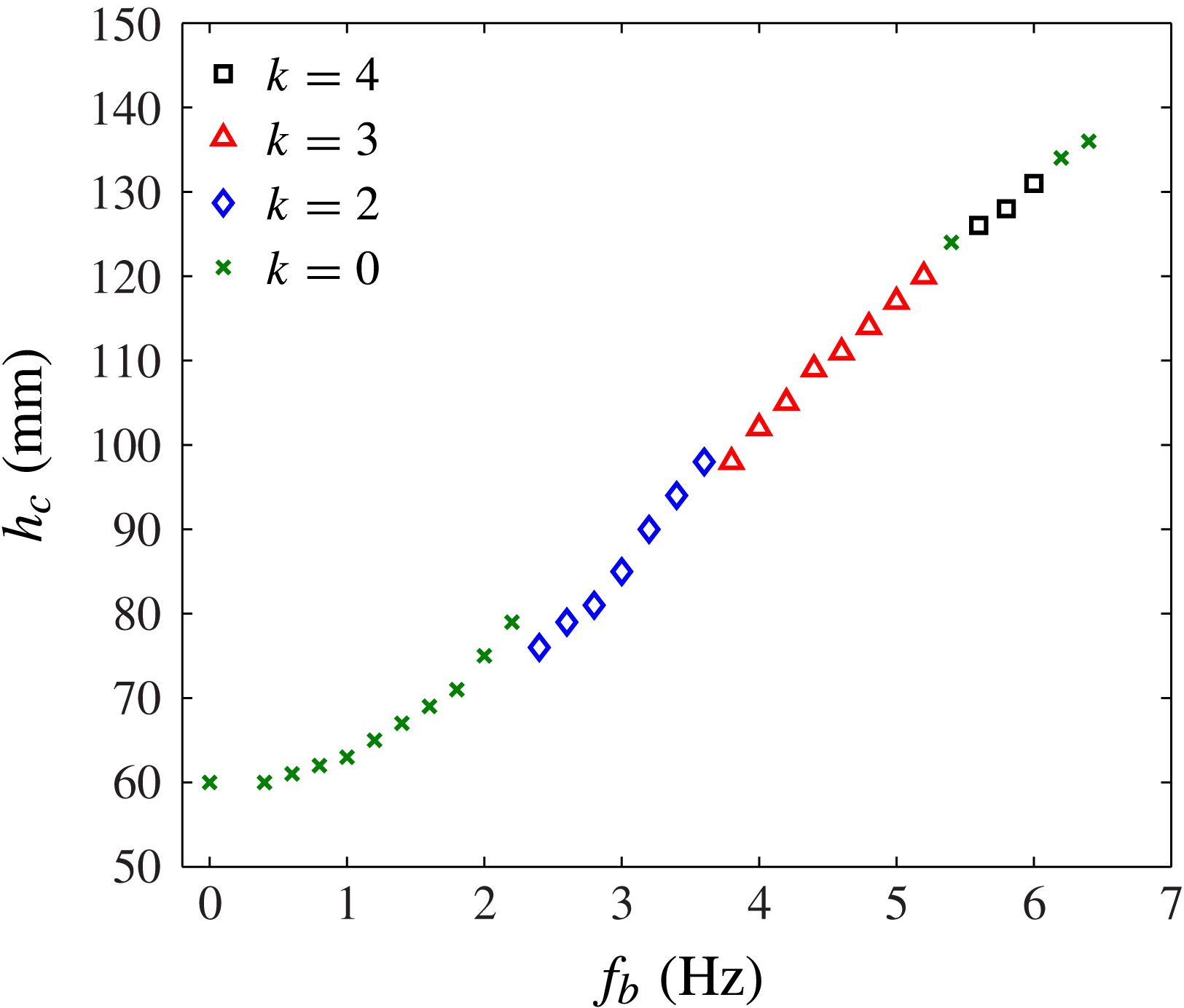
When the bottom is rotating the water is pushed out from the centre and up against the cylinder wall. The average water height at the cylinder wall,
 $h_{c}$
, shown in figure 2, is a measure of the velocity profile. If the flow is close to a line vortex as claimed by Tophøj et al. (Reference Tophøj, Mougel, Bohr and Fabre2013) this height would determine the circulation. In figure 5 we plot the values of
 $h_{c}$
against
 $f_{b}$
for
 $H=60\ \text{mm}$
, i.e. one of the columns in figure 4. The curve is continuous, except at the rotational frequencies where the number of corners change, and even there the change is only a few millimetres. It is interesting that the jumps are always downwards, so one might speculate that the system gains potential energy by adding corners at the appropriate rotational frequency.
The average height of the water at the cylinder wall,
 $h_{c}$
as function of the bottom plate frequency,
 $f_{b}$
. The cylinder wall was stationary,
 $f_{c}=0\ \text{Hz}$
and the filling height of the water was
 $H=60\ \text{mm}$
.

4. Combining bottom and cylinder rotation
We now rotate both the bottom plate and the cylinder independently with frequencies
 $f_{b}$
and
 $f_{c}$
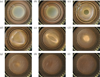
, respectively. In figure 6 we show snapshots taken from above of the states going from Newton’s bucket,
 $f_{b}=f_{c}$
(figure 6
a) to the case
 $f_{b}=-f_{c}$
(figure 6
i), where the bottom and cylinder counter-rotate with the same frequency, by slowly decreasing the cylinder frequency while keeping the bottom frequency constant at
 $f_{b}=2\ \text{Hz}$
. We simply decrease
 $f_{c}$
by 0.4 Hz between each snapshot and these do therefore not necessarily show the clearest polygons. In figure 6(b) we still see no polygon, just a ‘dry’ circular state. The first polygon, a square, forms at
 $f_{c}=0.8\ \text{Hz}$
(figure 6
c). It is ‘wet’ in the sense that the square contour is covered by water, but it has a dry circular centre. The square transforms into a wet triangle at
 $f_{c}=0.4\ \text{Hz}$
(d), and then a wet ellipse at
 $f_{c}=0\ \text{Hz}$
(e). When
 $f_{c}$
becomes negative (counter-rotation) the ellipse is destroyed and only a central dent in the surface is left ( f) and (g), which becomes smaller and smaller until the water surface seems completely flat (h) and (i). The extreme states, i.e.
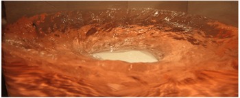
 $f_{b}=f_{c}$
and
 $f_{b}=-f_{c}$
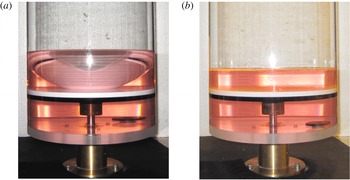
, are shown from the side in figure 7(a,b), respectively, in this case, for
 $f_{b}=4\ \text{Hz}$
, but with the same filling height (
 $H=40\ \text{mm}$
). In the latter case the surface deformation is nearly invisible, despite being disordered by turbulent fluctuations.
Snapshot of the surface states at
 $H=40\ \text{mm},f_{b}=2.0\ \text{Hz}$
, and: (a)
 $f_{c}=2.0\ \text{Hz}$
, Newton’s bucket; (b)
 $f_{c}=1.2\ \text{Hz}$
, circle; (c)
 $f_{c}=0.8\ \text{Hz}$
, square; (d)
 $f_{c}=0.4\ \text{Hz}$
, triangle; (e)
 $f_{c}=0\ \text{Hz}$
, ellipse; ( f)
 $f_{c}=-0.4\ \text{Hz}$
, central surface dent; (g)
 $f_{c}=-0.8\ \text{Hz}$
, central surface dent; (h)
 $f_{c}=-1.2\ \text{Hz}$
, flat; and (i)
 $f_{c}=-2.0\ \text{Hz}$
, flat.

(a) Newton’s bucket flow,
 $f_{b}=f_{c}=4\ \text{Hz}$
, where the water is pushed outward from the centre due to the centrifugal force. (b) Here
 $f_{b}=-f_{c}=4\ \text{Hz}$
, and the average water surface is flat, but with strong turbulent fluctuations since the rotation of the cylinder counteracts the influence of the rotation of the bottom plate. In both cases
 $H=40\ \text{mm}$
.

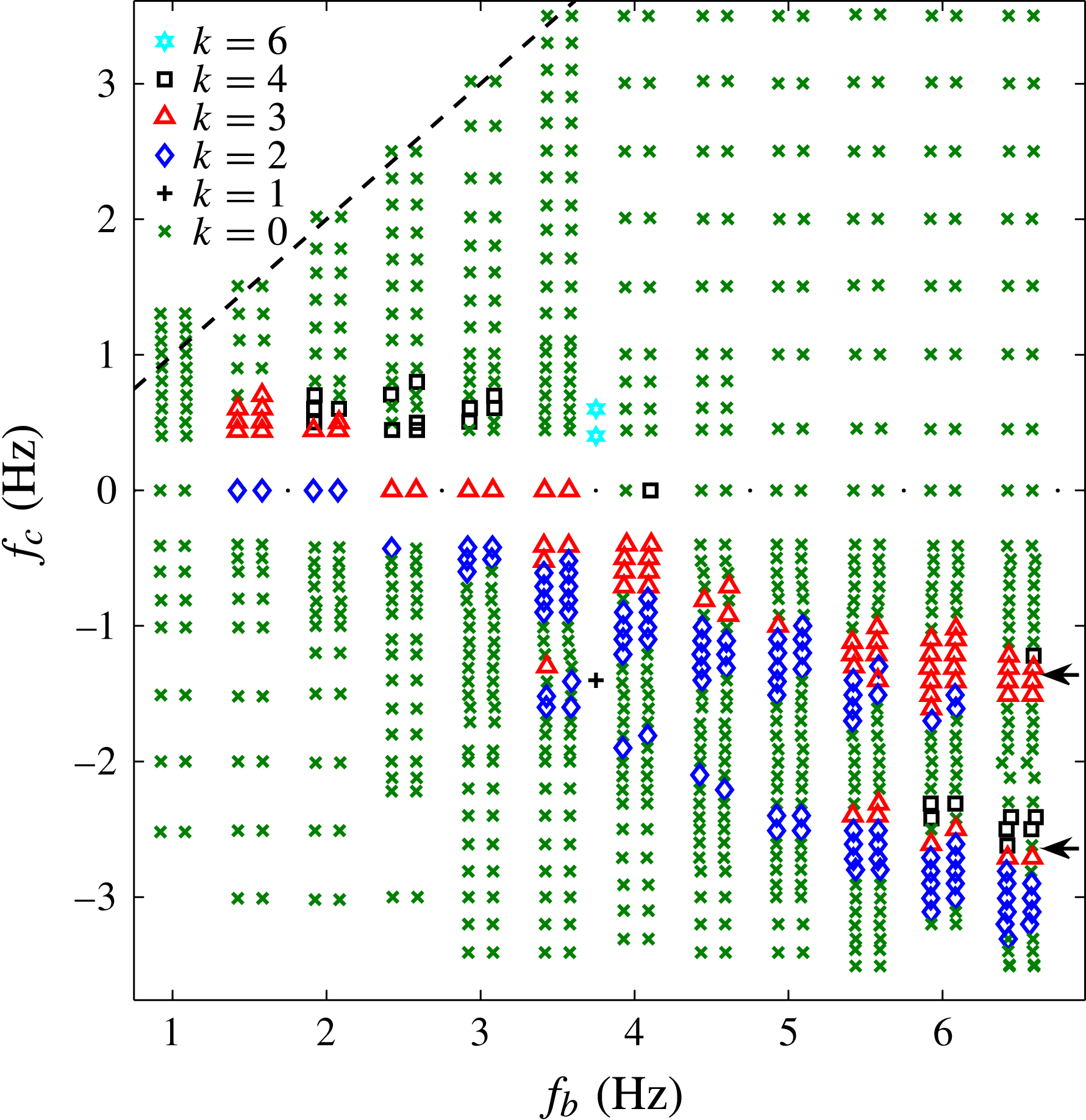
In figure 8 we show a phase diagram spanned by
 $f_{b}$
and
 $f_{c}$
, where we have fixed the filling height at
 $H=40\ \text{mm}$
, for which we know from figure 4, that there is a large range of stable states when
 $f_{c}=0$
. The bottom frequency
 $f_{b}$
was set between 1.0 and 6.5 Hz with steps of 0.5 Hz, and for each of these values
 $f_{c}$
was varied with steps of 0.1 Hz. Negative values of
 $f_{c}$
indicate that the cylinder is rotating in the opposite sense of the bottom. Note that the horizontal data line for
 $f_{c}=0$
is the same as the vertical data line for
 $H=40\ \text{mm}$
in figure 4. The dashed black line is the Newton’s bucket flow
 $f_{c}=f_{b}$
.
Phase diagram of the states at
 $H=40\ \text{mm}$
for variable
 $f_{b}$
and
 $f_{c}$
. We have not distinguished between ‘wet’ and ‘dry’ cases. The majority of the polygonal states are found when the cylinder rotates in the opposite direction to the bottom plate. The lower band of states has no counterpart in the system, where only the bottom rotates and has not to our knowledge been described before. The states marked by the arrows are shown in figure 9 which highlight the difference between the two bands. We find hexagons on the line
 $f_{b}=3.75\ \text{Hz}$
and also a monogon (
 $k=1$
) (see figure 11).

As expected, and confirmed theoretically by Fabre & Mougel (Reference Fabre and Mougel2014), we see no instability at or near the rigidly rotating flow, which appears like a perfect glass bowl (figures 6
a and 7
a). Actually, the polygonal states lie in a wedge-shaped region with predominantly negative values of
 $f_{c}$
. For a given bottom frequency the order of appearance of the polygonal states, when the cylinder frequency is increased, is similar to that we find with the stationary cylinder, and thus we have the same order both vertically and horizontally. From the bottom it is first ellipses; then triangles and then squares, although some shapes are missing for some bottom frequencies. The regions with the same polygonal state are shifted downward in the phase diagram for increasing bottom frequency. For an increase in
 $f_{b}$
of 1 Hz the area of, e.g., triangles is shifted down by approximately 0.3 Hz in
 $f_{c}$
.
An interesting new feature is the existence of two bands of polygons in figure 8. The lower band only exists at negative
 $f_{c}$
and comes into being at
 $f_{c}\approx 1.5\ \text{Hz}$
, and thus has no analogue in the
 $f_{c}=0$
phase diagram in figure 4. These polygons are smaller than those in the upper band with cylinder frequencies closer to zero, as shown in figure 9. In contrast, polygons in the same band with the same
 $k$
are known to be different, but predominantly in angles and shapes; not in size (Vatistas Reference Vatistas1990). Just like in the case of the polygons with stationary cylinder, the polygons rotate in the same direction as the bottom plate. Surprisingly, the two triangles in figure 9 have essentially the same rotational frequency,
 $f_{p}=(1.15\pm 0.05)\ \text{Hz}$
, despite their very different sizes and cylinder frequencies that differ by a factor close to two.
Triangles in the two bands at
 $f_{b}=6.5\ \text{Hz}$
and
 $H=40\ \text{mm}$
(see arrows in figure 8): (a) at
 $f_{c}=-1.4\ \text{Hz}$
(upper band) and (b)
 $f_{c}=-2.6\ \text{Hz}$
(lower band). The shapes of the polygons in the two bands are similar, but their linear size differs roughly by a factor of two. Both polygons rotate in the same direction as the bottom plate, and with similar frequencies,
 $f_{p}=(1.15\pm 0.05)\ \text{Hz}$
.

An interesting flow is seen in the second band when cylinder and bottom plate counter-rotate at high frequencies. Here, an annular transition region in the flow and surface height is present approximately 4 cm from the cylinder wall (figure 10). Another unexpected feature of combining bottom plate and cylinder rotation in opposing directions, is the appearance of a dry ‘monogon’, a state with
 $k=1$
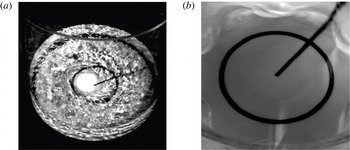
. The monogon is an eccentric circular hole which, contrary to all of the other polygons, rotates in the opposite sense of the bottom plate, i.e. with the same sense as the cylinder. It is shown in figure 11(a) and can be seen ‘live’ in the movie provided in the supplementary material available at http://dx.doi.org/10.1017/jfm.2014.568. Further, we see hexagons (figure 11
b), as shown in the phase diagram figure 8, at
 $f_{b}=3.75\ \text{Hz}$
, when the cylinder is slightly co-rotating.
Annular transition region when bottom plate and cylinder counter-rotate.

(a) The monogon is roughly an eccentric circle rotating around the centre of the container. It is found near the plus sign in figure 8. The central black circle was painted on the bottom plate. The picture is a snapshot from the movie in the supplementary material. (b) The hexagon from the phase diagram in figure 8.

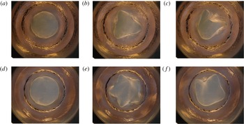
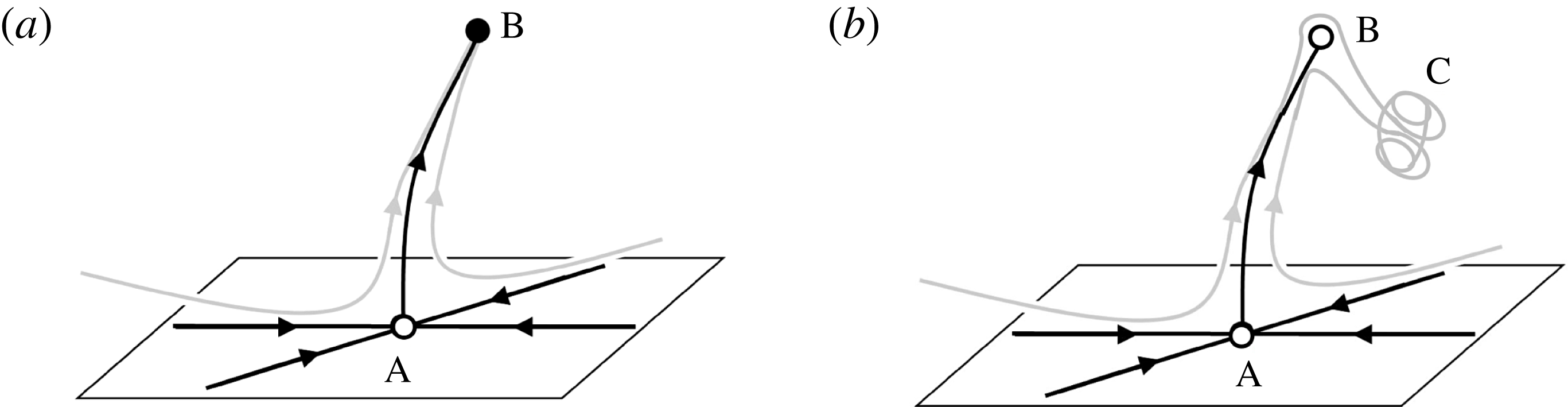
It also happens, typically near the transition lines, that the system never settles on a stationary state but remains in an unsteady state of which examples are shown in figure 12. Bergmann et al. (Reference Bergmann, Tophøj, Homan, Hersen, Andersen and Bohr2011) showed that the formation of a stationary polygonal state can take place via a circular state, and these states are represented as fixed points in figure 13(a). Since the system initially approaches the circular fixed point ‘A’, it must have many stable directions; although it finally turns out to be a saddle point with a well-defined unstable manifold as sketched in figure 13(a), taking the system off in the direction of the polygon. Similarly the creation of the deformed, non-stationary ‘polygons’ seems to take place via first the circular state (figure 12(left)), the saddle point ‘A’, and then the polygon ‘B’ in figure 13(a) (e.g. the triangle and pentagon shown in figure 12(centre), which now has turned into a weakly unstable saddle point controlling the approach to the final state (figure 12(right))), which, in this case, is not a fixed point, but a non-stationary state represented by something like a strange attractor at ‘C’ in figure 13(b).
Time series of the formation of an unstable triangle (a) and an unstable pentagon (b). First the flow approaches a circular state (left), then it settles on a regular polygonal state (centre), but after a few seconds it becomes irregular (right) and never settles down. The triangle is found at
 $f_{b}=4.0\ \text{Hz}$
,
 $f_{c}=0.44\ \text{Hz}$
and
 $H=60\ \text{mm}$
, and the pentagon at
 $f_{b}=4.0\ \text{Hz}$
,
 $f_{c}=1.2\ \text{Hz}$
and
 $H=70\ \text{mm}$
.

(a) Phase space for the development of a polygonal state. Initially the system moves towards an almost stable circular shape, A. The fact that A is unstable is felt only very close to it, so from the vicinity of A the system goes off on a well-defined unstable manifold towards a regular stable polygon, B (Bergmann et al. Reference Bergmann, Tophøj, Homan, Hersen, Andersen and Bohr2011). (b) Development of the system, when the polygon has become slightly unstable. First it moves toward a circular shape, A, thereafter toward the polygon, B, before it goes off toward something resembling a strange attractor, C, where it remains without settling in a stable state.

5. Rotation rate and phase of the polygons
We now return to the case in which only the bottom plate rotates and we shall compare our results with earlier studies. In the experiments by Suzuki et al. (Reference Suzuki, Iima and Hayase2006) and Tasaka & Iima (Reference Tasaka and Iima2009) the cylinder radius was much smaller than in our set-up and the focus was on states with surface switching. In the experiments by Vatistas (Reference Vatistas1990) and Vatistas et al. (Reference Vatistas, Wang and Lin1992) there were a large annular gap between the rotating bottom plate and the cylinder (42 mm and 16 mm, respectively), in contrast to the small gap in our set-up (1 mm). The size of the cylinders in the three experiments are however similar (285 and 290 mm). Since the geometry in one of the set-ups in the work by Jansson et al. (Reference Jansson, Haspang, Jensen, Hersen and Bohr2006) is the same as in the present experiment and those of Vatistas (Reference Vatistas1990) and Vatistas et al. (Reference Vatistas, Wang and Lin1992) are comparable, we shall restrict our quantitative comparison with earlier results to these works. We note that in the paper by Jansson et al. (Reference Jansson, Haspang, Jensen, Hersen and Bohr2006), which was co-authored by one of us (T.B.), the inner diameter of the cylinder was incorrectly reported to be 26.2 cm, but in fact it was 29.0 cm.
Phase diagram for
 $f_{c}=0$
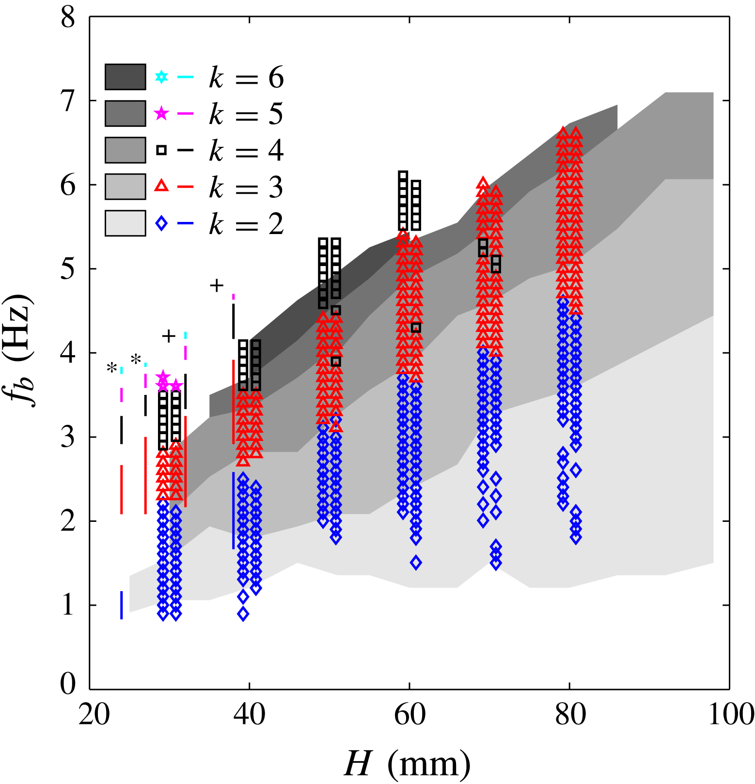
with the data in figure 4 (symbols) overlayed on the data by Jansson et al. (Reference Jansson, Haspang, Jensen, Hersen and Bohr2006) (greyscale), and with Vatistas (Reference Vatistas1990) (+) and Vatistas et al. (Reference Vatistas, Wang and Lin1992) (*) shown as straight coloured lines.

In figure 14 the data from figure 4 is plotted with the data from Vatistas (Reference Vatistas1990), Vatistas et al. (Reference Vatistas, Wang and Lin1992) and Jansson et al. (Reference Jansson, Haspang, Jensen, Hersen and Bohr2006). Our phase diagram agrees qualitatively with Jansson et al. (Reference Jansson, Haspang, Jensen, Hersen and Bohr2006), but there are quantitative differences. All of the threshold values are at higher rotational frequencies in our set-up. For example, the band of triangles has been pushed up by approximately 1 Hz. As can also be seen, Jansson et al. (Reference Jansson, Haspang, Jensen, Hersen and Bohr2006) found more polygonal states than we do. We only find pentagons for
 $H=30\ \text{mm}$
, which, incidentally, is the only filling height where they do not find pentagons. Further, they do find hexagons, which we do not unless the cylinder is rotating. The four coloured lines in figure 14 indicate the results from Vatistas (Reference Vatistas1990, figure 8) and Vatistas et al. (Reference Vatistas, Wang and Lin1992, figure 6). As can be seen, their results are also similar to ours. In Vatistas et al. (Reference Vatistas, Wang and Lin1992) the water level was 24 and 27 mm and the gaps between the stationary states in their diagram are significantly larger than ours. The threshold frequencies for polygonal states are higher in Vatistas (Reference Vatistas1990), in particular for
 $k=4$
to
 $k=6$
.
We do not understand the appreciable quantitative differences between the various results shown in the figure. In particular, the results of Jansson et al. (Reference Jansson, Haspang, Jensen, Hersen and Bohr2006) should be completely compatible with ours. In their experiment, the bottom plate had a vertical wobble motion of approximately 2 mm, whereas ours is less than 0.5 mm. Could the larger misalignment in Jansson et al. (Reference Jansson, Haspang, Jensen, Hersen and Bohr2006) actually excite and stabilise the polygonal states by a continuing asymmetrical forcing? To answer this we shall provide measurements of the rotational frequencies of the figures and detailed comparison with the rotational frequencies of the plate.
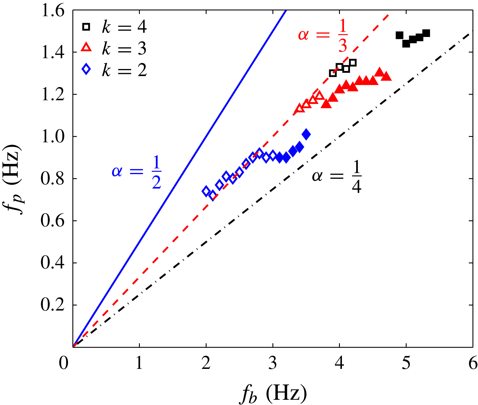
In figure 15 we show the rotation frequencies
 $f_{p}$
of some of the polygons as function of the plate frequency
 $f_{b}$
at a filling height of
 $H=50\ \text{mm}$
. Here we have distinguished between ‘wet’ polygons, where the bottom plate is entirely covered by water (open symbols) and ‘dry’ polygons, where there is a dry central region (filled symbols). If periodic forcing is important, we would expect signs of phase-locking between the bottom plate and the rotating polygon, and we should thus look for rational ratios between
 $f_{b}$
and
 $f_{p}$
. As seen in figure 15, some of the triangles (in this case the wet ones) have a ratio very close to
 $\frac{1}{3}$
, which means that the triangle rotates approximately one corner for every full rotation of the bottom plate and could imply phase-locking between plate and triangle.
The rotational frequency of the polygons,
 $f_{p}$
, as function of the rotational frequency of the bottom plate,
 $f_{b}$
, with constant water filling height,
 $H=50\ \text{mm}$
. The dry states have filled markers and the wet states have open markers. The straight lines have the slopes
 $\frac{1}{2}$
(solid),
 $\frac{1}{3}$
(dashed) and
 $\frac{1}{4}$
(dashed-dotted).

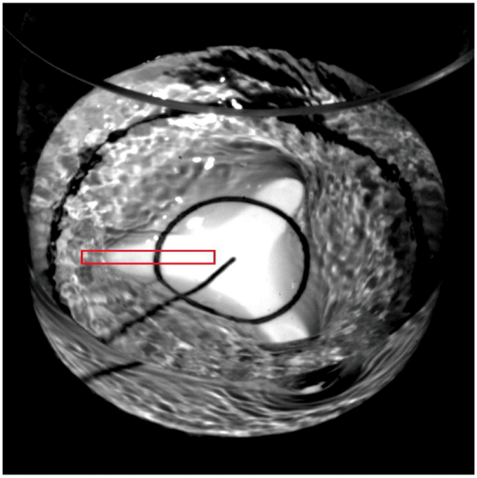
To investigate whether the phase of the polygons are actually locked to that of the plate, we have measured their phases accurately. Since it is easier to monitor dry triangles (due to larger contrast), we have decreased the filling height slightly to
 $H=40\ \text{mm}$
, where dry triangles with a frequency ratio very close to
 $\frac{1}{3}$
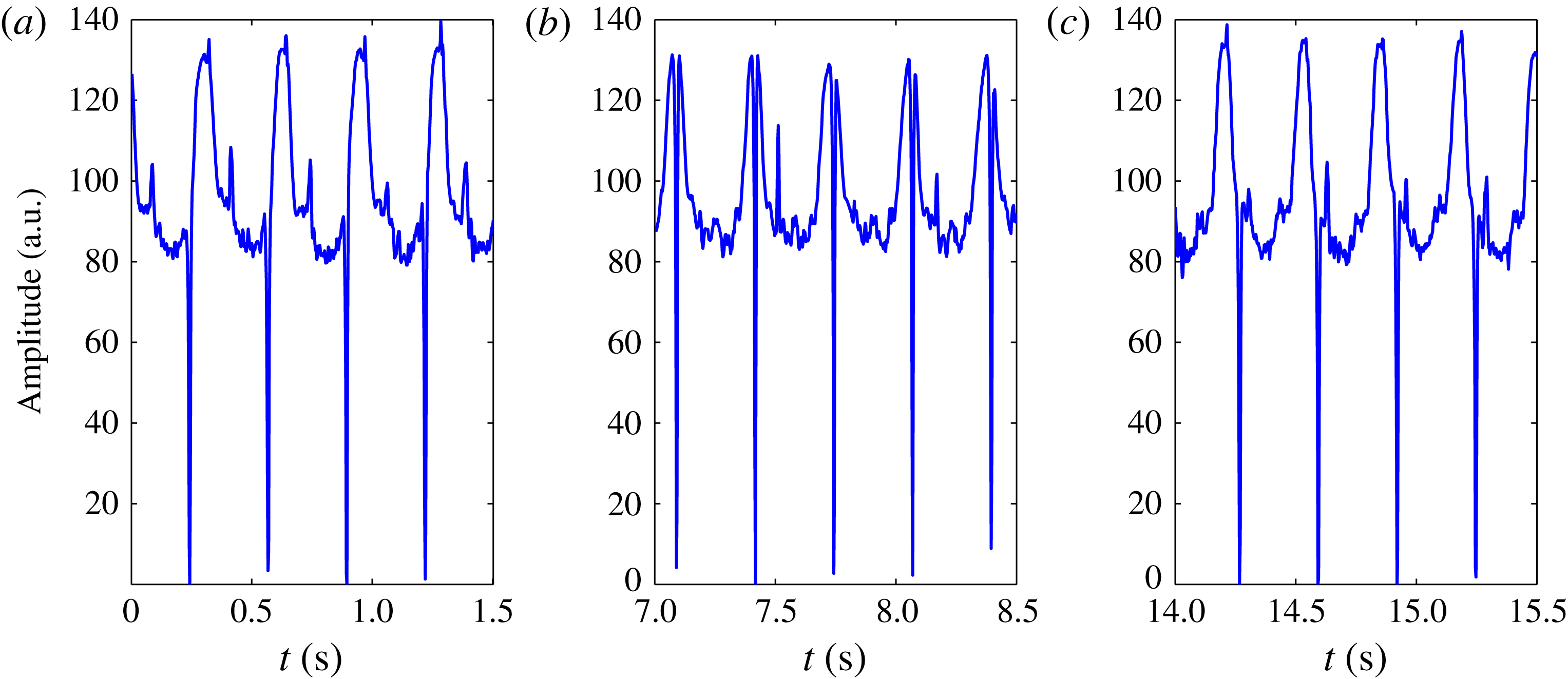
are found. To monitor the phases we make a high-speed recording of the experiment from above. One frame of the resulting movie is shown in figure 16, and it can be seen that the white bottom plate has been painted with a black central circle and a black radial line. To extract quantitative results from the movies, the average value of the pixel intensities in the (red online) box is taken for every frame. If an arm of the triangle is in the (red online) box, this value will be high because a lot of white bottom plate is reflecting the light. That is the case in figure 16. If the arm is not in the (red online) box, the value will be lower. This gives a measure for the phase and amplitude of the distortion wave. The rotation of the bottom plate can be monitored similarly because for each period, the radial line painted on the bottom plate will pass through the (red online) box once. When it does, the average pixel value will be very low because the line is black.
Picture from video used to extract the frequency
 $f_{b}$
of the bottom plate and the frequency
 $f_{p}$
of the polygon, in this case the triangle at
 $H=40\ \text{mm}$
and
 $f_{b}=3\ \text{Hz}$
. The plate for this study was painted with a radial line. The average value of the pixels in the (red online) box were used as an indicator of the position of both the figure and the bottom.

In figure 17 one can see the results of a measurement of the distortion wave and the bottom plate. As can be seen, the frequency of the figure is close to
 $\frac{1}{3}$
of that of the bottom plate. However, the ratio is not exactly
 $\frac{1}{3}$
and they are not phase locked. The figure shows recordings of the phase of the figure and that of the plate over around 45 rotations of the plate and in this time the phase difference varies by around
 ${\rm\pi}$
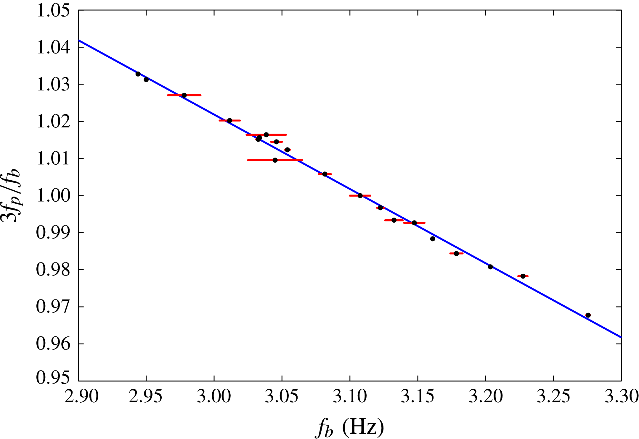
. Also, there seems to be no sign of interference between the figure rotation and that of the bottom plate: the amplitude and the distance between two peaks of the polygon remains close to constant throughout the experiment. Figure 18 shows the frequency of the polygon (multiplied by three) divided by that of the bottom plate versus the frequency of the bottom plate. If there was phase locking, plateaus with constant frequency ratio would appear, but within the accuracy of our experiment they were not seen. We have tested this conclusion with irregularities in the form of ‘bumps’ glued on the plate to create a kind of artificial wobbling. Again, we never found phase locking.
The amplitude of the distortion wave describing the triangle and the position of the black radial line on the bottom plate versus time for
 $H=40\ \text{mm}$
and
 $f_{b}=3\ \text{Hz}$
. The vertical lines going all of the way down signify the black radial line on the bottom plate, whereas the softer upward peaks represent one ‘arm’ or corner of the triangle passing the (red online) box. Taking the three pictures separately, it seems that bottom plate and polygon are phase locked, but combining them it can be seen that they are not, i.e. the phase of the figure is drifting relative to the bottom plate.

Frequency ratio of the polygonal state and the bottom plate, versus frequency of the bottom plate close to the case
 $f_{p}/f_{b}=\frac{1}{3}$
with water filling height
 $H=40\ \text{mm}$
. It is seen that the frequency-locked case
 $f_{p}/f_{b}=\frac{1}{3}$
is not preferred over values close by. The dots are the measurement points, the line is a fit and the horizontal lines show the extent of the variation in frequency of the bottom plate during the measurements.

6. Multistability and excitability
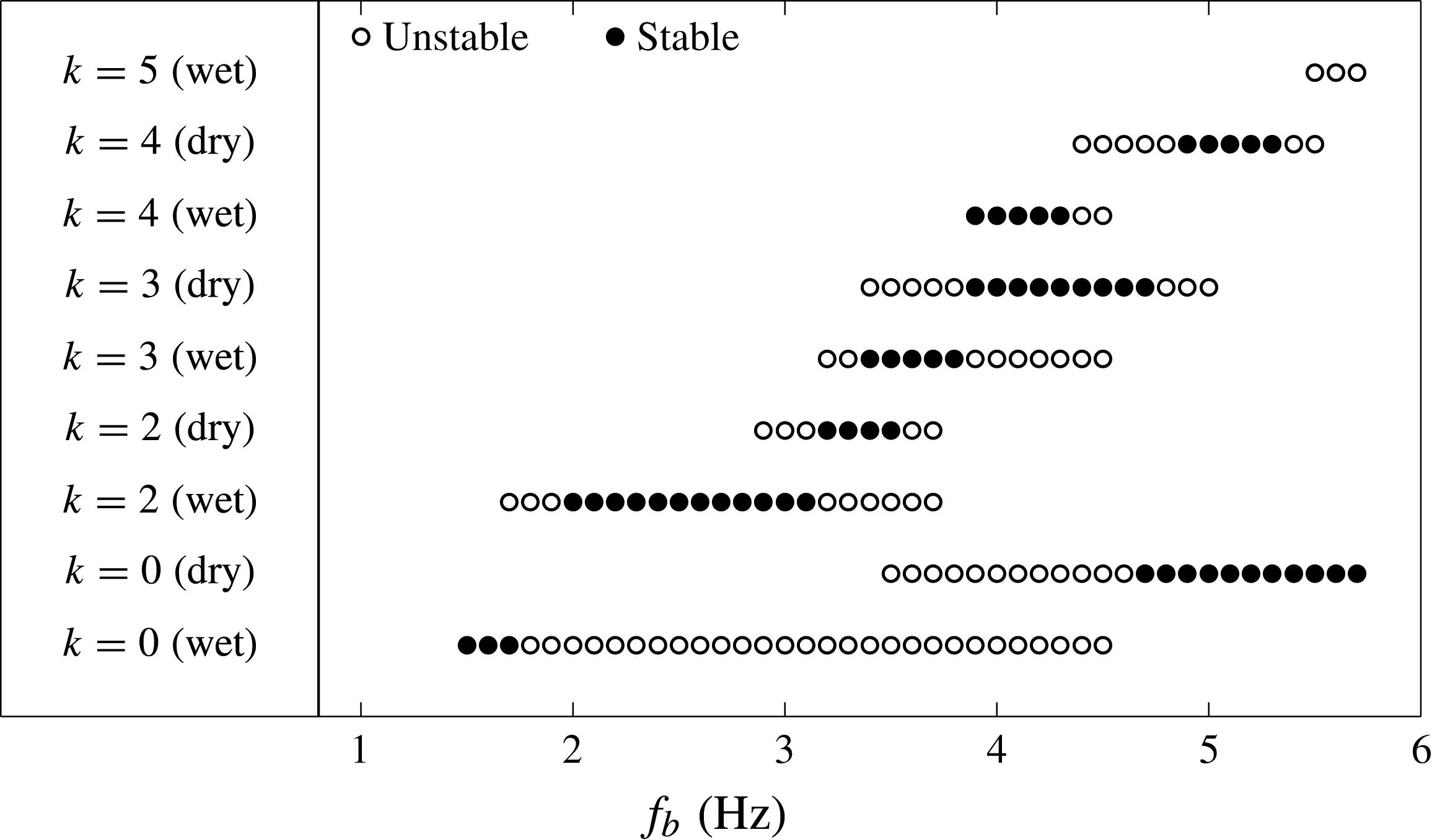
Bistability and hysteresis was found in the experiments by Vatistas (Reference Vatistas1990), Jansson et al. (Reference Jansson, Haspang, Jensen, Hersen and Bohr2006) and Vatistas et al. (Reference Vatistas, Abderrahmane and Kamran Siddiqui2008), and such phenomena have also been reported for the states with surface switching in the experiments by Tasaka & Iima (Reference Tasaka and Iima2009). In our experiment the surface states show a considerable multi-stability, which is hard to capture in a phase diagram. For most parameters, we find a unique stable state, independently of whether the flow was started from rest or from another state or was perturbed by stirring the flow. However, at certain frequencies two or several final states are observed. This happens at the transitional frequencies, where the system changes polygonal state, and there the final state seems rather unpredictable and dependent on small changes in the initial conditions.
In addition to the stable states there are a number of ‘virtual’, almost stable states, which can be excited by slightly perturbing the flow. One way of doing this is to insert a flat, rigid plate vertically into the flow near the rim. According to Tophøj et al. (Reference Tophøj, Mougel, Bohr and Fabre2013), the instability forming the polygons stems from resonances between the gravitational waves near the rim of the cylinder and the ‘centrifugal’ waves near the centre, and the inserted plate seems to increase the interaction between these waves. As an example, we show in figure 19 the states that we have observed at a filling height of
 $H=50\ \text{mm}$
, where the stable states are marked with filled symbols and the unstable states are marked with open symbols. One can see that at frequencies near
 $f_{b}=3.5\ \text{Hz}$
, it is possible in this way to obtain six different states. We have perturbed the flows both with a ruler held by hand, and with a ruler mounted on a motor, which could flap it along its vertical axis with a given frequency, but the perturbing frequency did not seem to have any strong influence on the possible states. As can be seen, a circular state is always, at least almost stable, as also pointed out by Bergmann et al. (Reference Bergmann, Tophøj, Homan, Hersen, Andersen and Bohr2011), and it is interesting to note that even this simple state is not unique, since, for some parameters (e.g. around
 $f_{b}=4\ \text{Hz}$
), we can have both a wet and a dry circular state coexisting.
Phase diagram with both stable and unstable shapes at filling height
 $H=50\ \text{mm}$
. The bottom frequency is along the abscissa and the ordinate shows the appearing shapes at this frequency. Note that the circular state exists at all bottom frequencies.

It thus appears that the stability and appearance of the polygons can depend strongly on details in the experiment. One such detail, which should be studied more carefully in the future, appears to be the temperature. Our preliminary observation show that fewer polygons appear in warm water than in cold water, which probably means that even small changes in viscosity, say, of the order of 30 %, can have an important effect on the stability.
7. Conclusions
We have presented experimental observations of ‘polygons’ on a free fluid surface in a cylindrical container, where the frequency of the bottom plate and the cylinder walls can be varied independently. We have shown that the polygonal instability sets in at some distance from the Newton’s bucket flow and that the polygons fall in two distinct families: those with low rotation rates of the cylinder, which are related to those found earlier and those at large counter-rotation rates which form a new family of smaller sizes. We have compared the case of a stationary cylinder with earlier work (Vatistas Reference Vatistas1990; Vatistas et al.
Reference Vatistas, Wang and Lin1992; Jansson et al.
Reference Jansson, Haspang, Jensen, Hersen and Bohr2006) and we find qualitatively similar phase diagrams but considerable quantitative differences. Thus, the triangles in our system are found approximately 1 Hz higher than in Jansson et al. (Reference Jansson, Haspang, Jensen, Hersen and Bohr2006), and we found fewer pentagons and no hexagons as long as the cylinder is stationary. We showed that a triangle rotating at a rate very close to
 $\frac{1}{3}$
of the rotation rate of the plate, has a phase which is not locked to that of the plate, and we conclude that the instability is apparently not driven by small misalignments in our set-up.
For the two-frequency system, we found an additional novel state, a monogon with one ‘corner’ roughly an eccentric circle rotating in the same sense as the cylinder and opposite to that of the plate. The system also displays a considerable multi-stability, in particular near transition points, and we showed that it is possible to excite ‘virtual’ polygons by inserting a plate vertically in the flow. This means that the stability properties of the polygons are strongly dependent on details in the experiment and small external perturbations.
Acknowledgements
We are grateful to R. Kerswell for suggesting an experiment with independent control of the bottom and cylinder rotations and to L. Tophøj, J. Mougel and D. Fabre for discussions of our results. We are also grateful to K. A. Mørch and E. Hansen for helping us with the design of the set-up and to E. Hansen for his careful work in constructing the set-up. We would like to thank Brdr. Hartmann’s Foundation for a grant, which allowed us to build the experiment.
Supplementary movie
Supplementary movie is available at http://dx.doi.org/10.1017/jfm.2014.568.