



1. Introduction
Over the last three decades, wind power has emerged as a crucial renewable energy source, expected to supply up to half of global electricity demand by the midcentury (Kaldellis & Zafirakis Reference Kaldellis and Zafirakis2011; McKenna et al. Reference McKenna2025). While horizontal-axis wind turbines dominate energy production, vertical-axis wind turbines (VAWTs) have seen a surge in popularity, because of their (i) omnidirectional operation, (ii) improved scalability, (iii) simpler maintenance and (iv) lower noise levels. These reasons render them excellent complements to their horizontal counterparts, in particular in urban turbulent flows (Rezaeiha et al. Reference Rezaeiha, Kalkman and Blocken2017; Rolin & Porté-Agel Reference Rolin and Porté-Agel2018). However, the complex aerodynamics of VAWTs limits efficiency and reliability, ultimately impeding widespread adoption (Kumar et al. Reference Kumar, Raahemifar and Fung2018).
Numerous studies have therefore sought to enhance understanding of the complex physical phenomena at play in this context. These works (Fujisawa & Shibuya Reference Fujisawa and Shibuya2001; Simão Ferreira et al. Reference Simão Ferreira, Bijl, van Bussel and van Kuik2007; Sutherland, Berg & Ashwill Reference Sutherland, Berg and Ashwill2012) revealed that VAWT blades undergo substantial variations in flow conditions, characterised by the effective velocity and angle of attack. Large excursions of these parameters can lead to dynamic stall (Mulleners & Raffel Reference Mulleners and Raffel2013; Dunne & McKeon Reference Dunne and McKeon2015). The most critical conditions are found during the upwind half of a cycle, where vortices are shed from the leading edge of the blade, causing a drastic drop in forces and significant load fluctuations. The released vortex then convects downstream and, for some combinations of non-dimensional governing parameters (i.e. Reynolds number
 $\textit{Re}$
, chord-to-diameter ratio
 $c/D$
and tip-speed ratio
 $\lambda$
), interacts with the blade on its downwind trajectory, further reducing the turbine’s efficiency. For instance, Laneville & Vittecoq (Reference Laneville and Vittecoq1986) and Wang et al. (Reference Wang, Sun, Zhu, Zhang and Huang2016) showed that dynamic stall occurs at tip-speed ratios below 4, while Buchner et al. (Reference Buchner, Soria, Honnery and Smits2018) highlighted its industrial relevance, noting that VAWTs typically achieve peak aerodynamic performance within this range. It presents a trade-off: operating at low tip-speed ratios improves power output but also increases the severity of dynamic stall. Le Fouest & Mulleners (Reference Le Fouest and Mulleners2022) labelled this performance conflict as the dynamic stall dilemma.
In response, researchers have explored various flow control strategies aimed at altering flow dynamics at low tip-speed ratios. Proposed methods include finding an optimal preset blade pitch angle (Rezaeiha et al. Reference Rezaeiha, Kalkman and Blocken2017) or varying the blade pitch with a proportional-integral-derivative controller. Despite improvements, the nonlinear and unsteady dynamics of VAWTs make linear methods inadequate for fully exploiting the potential of active control (Abdalrahman et al. Reference Abdalrahman, Melek and Lien2017). More complex control functions are sought through trajectory planning methods, which attempt to optimise how an object moves along a given path. The cyclical nature of VAWTs logically leads to these movements being represented by trigonometric relations. For instance, Gosselin, Dumas & Boudreau (Reference Gosselin, Dumas and Boudreau2016) observed notable improvements with their proposed arctangent-based pitch function. Paillard et al. (Reference Paillard, Astolfi and Hauville2015) numerically evaluated various harmonics for pitch control and showed that a second harmonic profile significantly outperformed a fixed-pitch blade. Le Fouest & Mulleners (Reference Le Fouest and Mulleners2024) extended this concept in an experimental setting using an open-loop control approach, representing all harmonics in a single function optimised by a genetic algorithm. They demonstrated a three-fold power increase while reducing structure-threatening load fluctuations by
 $77\,\%$
. Flow control is not just limited to blade pitching, as demonstrated by Dave et al. (Reference Dave, Strom, Snortland, Williams, Polagye and Franck2021), who applied a sinusoidal variation to the angular velocity of the turbine, yielding substantial performance gains. The aforementioned strategies greatly increased understanding of the latent capabilities of VAWTs. However, these trajectory-based methods impose a control structure a priori, restricting the solution space to a prescribed functional form. They therefore rely on a degree of flow predictability that is rarely sustained in practice, especially as VAWTs get more integrated into the highly fluctuating urban wind environment. Furthermore, a fixed trajectory is incapable of responding to non-periodic flow variations, such as sudden gusts. This calls for a more adaptive control method that can respond in real time to changing aerodynamic conditions.
In that context, deep reinforcement learning (DRL) has recently emerged as a powerful framework for solving high-dimensional, nonlinear control problems. Among its notable achievements are: enabling continuous robotic control (Mahmood et al. Reference Mahmood, Korenkevych, Vasan, Ma and Bergstra2018), attaining superhuman performance in abstract strategy games such as Chess, Shogi and Go (Silver et al. Reference Silver2017), reducing traffic congestion through signal management (Tan et al. Reference Tan, Bao, Deng, Jin, Dai and Wang2020) and stabilising plasmas in tokamak reactors in real time (Degrave et al. Reference Degrave2022).
Despite DRLs great potential, its adoption into fluid mechanics has only recently begun to gain traction. An early implementation was presented by Rabault et al. (Reference Rabault, Kuchta, Jensen, Réglade and Cerardi2019), who demonstrated that a proximal policy optimisation agent could suppress vortex shedding in a von Kármán vortex street at a Reynolds number of 100 by adjusting the mass flow rates of two jets on the sides of a cylinder. Verma et al. (Reference Verma, Novati and Koumoutsakos2018) employed DRL to reveal optimal group swimming strategies at
 $\textit{Re} = 5000$
, where a follower fish learnt to exploit the leader’s wake, resulting in collective energy savings. Wang et al. (Reference Wang, Lin, Zhao, Chen, Guo, Yang, Wang and Fan2024) extended this concept by training an agent to flap an airfoil (at
 $\textit{Re} = O(10^3)$
), significantly enhancing efficiency and advancing the understanding of flapping motions. Their contribution also included investigations into various computational set-ups, highlighting DRLs sensitivity to the chosen algorithm and policy network architecture. Common issues in current active flow control applications include (i) excessive sensor requirements and (ii) limited insight into the agent’s learning behaviour. The former was addressed by Martin et al. (Reference Martin, Jardin, Rachelson and Bauerheim2024) who used the twin-delayed deep deterministic policy gradient (TD3) algorithm to mitigate gust-induced lift fluctuations using only onboard measurements as inputs. Along similar lines, Beckers & Eldredge (Reference Beckers and Eldredge2024) demonstrated how a TD3 agent outperforms standard linear controllers in various disturbed flow environments under partial observability, further highlighting the potential of DRL when sensing is restricted. Issue (ii) was explored in detail in a numerical study at
 $\textit{Re} = 100$
by Ren et al. (Reference Ren, Wang, Song and Tang2024), where DRL was applied to inhibit vortex-induced vibrations of a circular cylinder. Clear phases of the agent’s search path were identified and coupled to flow physics. The aforementioned studies have established a strong foundation for DRL in various fluid mechanics settings. Yet, application of DRL to VAWTs is still scarce. For instance, Soler et al. (Reference Soler, Marino, Huergo, Frutos and Ferrer2024) employed DRL coupled with blade element momentum theory to maximise wind turbine energy generation, showing significant improvements compared with proportional-integral–derivative controllers. In addition, Corban et al. (Reference Corban, Fernex, Mulleners, Rachelson, Bauerheim and Jardin2023) trained a DRL controller on a realistic VAWT operating in a water tunnel. While improvements were achieved, it remained suboptimal because of inherent noise and partial observation problems not fully elucidated yet. As a consequence, a missing step lies between DRL deployed on low-order models (Soler et al. Reference Soler, Marino, Huergo, Frutos and Ferrer2024) or realistic experiments (Corban et al. Reference Corban, Fernex, Mulleners, Rachelson, Bauerheim and Jardin2023) to evaluate the true potential of DRL in the presence of complex flows, as well as to identify the actual problems limiting the use of DRL in experimental set-ups. To bridge this gap, the present work couples DRL with unsteady simulations. Computational fluid dynamics (CFD) will capture more challenging physics compared with simplified low-order models. Moreover, this current use of DRL to VAWT constitutes an extent of current DRLs foundation to the domain of wind energy, where Reynolds numbers (here,
 $\textit{Re} = 4.52 {\times }10^4$
based on chord length and free stream velocity) are one to two orders of magnitude higher than previous works coupling DRL to CFD.
Thus, this paper presents a DRL framework for active flow control in VAWT, addressing the dynamic stall dilemma. Methodology is detailed in § 2, where a TD3 agent is coupled with a validated unsteady Reynolds-averaged Navier–Stokes (URANS) simulation. It is tasked with maximising power and limiting losses through mechanical actuation, while only receiving onboard information on airfoil pressure and position. Beyond final performance assessment, the framework’s training process is studied in § 3 to understand how control strategies develop. In particular, a comparison of the two controlled blades provides insight into the uniqueness of the optimal solution. Robustness of the DRL algorithm is evaluated by exposing the agent to varying inflow conditions. Finally, the power partitioning method (PPM) is used in § 4 to relate flow field changes to performance gains, thereby revealing the key physical mechanisms governing VAWT power production.
2. Vertical axis wind turbine simulation
2.1. Turbine kinematics
A two-bladed H-type Darrieus VAWT is studied. Its symmetry at the midsection in the vertical direction allows the turbine to be represented as a two-dimensional (2-D) problem with infinite aspect ratio blades. This approach removes relevant three-dimensional (3-D) aerodynamic effects such as the vortex stretching of shed vortices, spanwise flow divergence and losses due to the presence of tip vortices. Prior research has shown that 2-D models are capable of accurately reproducing the main physical flow phenomena while demonstrating reasonable agreement with experimental trends, despite sometimes overpredicting power output (Hansen & Sørensen Reference Hansen and Sørensen2001; Wang et al. Reference Wang, Ingham, Ma, Pourkashanian and Tao2010; Li et al. Reference Li, Zhu, Xu and Xiao2013; Rossetti & Pavesi Reference Rossetti and Pavesi2013). Moreover, the strong computational advantage is well suited for expensive control optimisation problems.
Vertical-axis wind turbine kinematics. (a) Schematic of variables. Note that the depicted
 $\alpha _{\!p}$
is positive while
 $\alpha _{\textit{eff}}$
is negative. (b) Effective flow variation throughout a turbine cycle for a blade pitched at
 $\alpha _{\!p} = 0^\circ$
.

Figure 1. Long description
Panel A: The schematic shows a vertical-axis wind turbine blade with various variables labeled. The blade is depicted with a chord length c and radius R. The angle of attack, alpha_p, is shown as positive, while the effective angle of attack, alpha_eff, is shown as negative. The velocity components U_infinity and U_eff are indicated, along with the rotational velocity Omega R. The angle theta is marked at the base of the blade. Panel B: The line graph illustrates the effective flow variation throughout a turbine cycle for a blade pitched at alpha_p equals 0 degrees. The x-axis represents the angle theta in degrees, ranging from 0 to 360. The left y-axis shows the effective angle of attack, alpha_eff, in degrees, ranging from -30 to 30. The right y-axis shows the normalized effective velocity, U_eff divided by Omega R, ranging from 0.5 to 1.5. The graph features two lines: one in pink representing alpha_eff and another in blue representing U_eff divided by Omega R. The pink line shows a sinusoidal pattern with peaks and troughs, while the blue line shows a complementary pattern.
Figure 1(a) shows a schematic diagram of one of the NACA 0018 airfoils in two different positions. During rotation, its quarter-chord point traverses a circular path of radius
 $R$
with a constant angular velocity
 $\varOmega$
. Here
 $\theta$
is the blade’s azimuthal position, which is
 $0^\circ$
at the top and increases in the anticlockwise direction. Time is reported in convective units
 $t^* = {U_\infty t}/{c}$
; accordingly, the convective cycle period is
 $T^* = ( {U_\infty }/{c})( {2 \pi }/{\varOmega })$
. The pitch
 $\alpha _{\!p}$
is defined as the angle between the tangential motion direction and the airfoil’s camber line, positive in clockwise direction. The VAWT kinematics are governed by the Reynolds number (
 $\textit{Re}$
), tip-speed ratio (
 $\lambda$
) and chord-to-diameter ratio (
 $c/D$
). The former two are defined as
 \begin{align} \textit{Re} = \frac {\rho U_\infty c}{\mu }, \qquad \lambda = \frac {\varOmega R}{U_\infty }, \end{align}
where
 $\rho$
and
 $\mu$
are the fluid’s density and dynamic viscosity, respectively. Here
 $\varOmega R$
is the velocity of the blade while
 $U_\infty$
is the free stream velocity. Throughout this study, the governing parameters remain fixed at
 $\textit{Re} = 4.52{\times }10^4$
,
 $\lambda = 1.9$
and
 $c/d = 0.24$
, as these values originate from the experiment (Snortland et al. Reference Snortland, Polagye and Williams2019) used to validate the simulation set-up.
In addition, the effective angle of attack
 $\alpha _{\textit{eff}}$
measures the angular distance between the effective flow velocity
 $U_{\textit{eff}}$
and the camber line which is positive in the anticlockwise direction. These are indicated in figure 1(a) and are defined as follows:
 \begin{align} \alpha _{\textit{eff}} &= \alpha _{\!p} - \tan ^{-1}\left (\frac {\sin \theta }{\lambda +\cos \theta }\right )\!, & U_{\textit{eff}}(\theta ) = U_\infty \sqrt {1+2\lambda \cos \theta + \lambda ^2}. \end{align}
These parameters render improved insights on what flow the airfoil perceives throughout a cycle. Note that they are purely derived from blade geometry and kinematics, so any wake effects altering the flow field are not included. Figure 1(b) displays the
 $\alpha _{\textit{eff}}$
and
 $U_{\textit{eff}}$
variation at a tip-speed ratio of 1.9. The combination of effective angles beyond the static stall regime and large flow velocity oscillations can lead to dynamic stall (Buchner et al. Reference Buchner, Soria, Honnery and Smits2018; Fouest & Mulleners Reference Le Fouest and Mulleners2022). This is generally coupled with an initial increase in blade loads as Mulleners & Raffel (Reference Mulleners and Raffel2013) demonstrated. However, large-scale vortex shedding, highly unsteady loads and eventually, drastic drops in forces, make dynamic stall undesirable. Equation (2.2) highlights the importance of pitch control, as
 $\alpha _{\!p}$
adjustments can restrict the
 $\alpha _{\textit{eff}}$
excursions in figure 1(b) to a smaller range and thus mitigate phenomena associated with dynamic stall.
During rotation, the blade experiences a total force
 $F_{\textit{tot}}$
and a pitching moment
 $M$
, computed at the quarter-chord point and defined as positive in the clockwise direction. The force
 $F_{\textit{tot}}$
can be decomposed into an azimuthal component
 $F_{\theta }$
, aligned with the blade’s motion, and a radial component
 $F_{R}$
, directed towards the origin. The azimuthal force contributes to the turbine’s power generation, as expressed by the power coefficient:
 \begin{equation} C_{\!p} = \frac {M_z \varOmega }{\frac {1}{2}\rho U_\infty ^3 A}, \quad \text{where} \quad M_z = F_\theta R. \end{equation}
Here
 $A = 2R$
which represents the 2-D area where the flow passes through the VAWT. Power is generated when
 $F_{\theta }$
produces a torque
 $M_z$
in the direction of turbine rotation. The coefficient
 $C_{\!p}$
is commonly understood as the conversion efficiency, as it is the ratio of total extracted power
 $P_{\textit{tot}}$
to the available wind power within the swept area. Note that (2.3) shows the non-dimensional power. Forces are instead non-dimensionalised by
 $C_{\!F} = {F}/({{1}/{2}) \rho U_{\infty }^2 A}$
.
2.2. Numerical method
The turbine motion and associated flow dynamics are simulated using CFD. The URANS equations are solved in Star-CCM + with a cell-centred finite volume method on the 2-D domain depicted in figure 2. It is composed of a
 $450c$
by
 $40c$
rectangular domain This replicates the experimental set-up of Snortland et al. (Reference Snortland, Polagye and Williams2019), as their data was used to validate the present simulations. The flow is driven by a velocity inlet with either a prescribed uniform flow of
 $U_\infty$
, or one of two shear profiles: upper side higher (USH) or lower side higher (LSH). In urban wind environments, horizontally asymmetric flows are commonly encountered (Wijayanto et al. Reference Wijayanto, Kono and Kiwata2020). Here, a linear profile serves as a first-order approximation to study the potential of DRL in these asymmetric circumstances. The USH profile increases the inlet velocity linearly from the lower boundary to the upper boundary while maintaining a reference velocity of
 $U_\infty$
at the turbine centre. The gradient direction is reversed in the LSH case. For both shear flows, the turbine simultaneously experiences an inflow velocity that is reduced by 9.4 % relative to
 $U_\infty$
on one side of the rotor and increased by 9.4 % on the opposite side. This is sufficient to alter the timing of dynamic stall and necessitate changes in pitching strategy. Furthermore, a pressure outlet is applied, along with slip walls for top and bottom boundary conditions. Each airfoil is embedded within an overset mesh that accounts for the combined VAWT solid-body rotation at
 $\varOmega$
and the blade’s pitch motion used for control.
Schematic overview of the computational domain. Dashed lines are used to indicate a zoomed-in view of the VAWT section.

The domain is discretised with a total of 120 000 cells, of which each overset mesh contains 30 000 cells. Prism layers at the airfoil walls yield the first cell at
 $\Delta y/c = 7.5{\times }10^{-4}$
to target
 $y^+$
values around or below 1.0. A finer mesh of 2
 ${\times }10^6$
cells, required for the proper computations of the PPM method, is used to analyse the optimal pitching policy in § 4. The temporal discretisation is chosen such that 312 time steps are taken per turbine revolution (
 $\Delta t = T/312$
). This set-up is implemented using second-order accurate schemes in both space and time. Contrary to typical practice in URANS simulations of VAWT (Raciti Castelli et al. Reference Raciti Castelli, Pavesi, Battisti, Benini and Ardizzon2010; Gosselin et al. Reference Gosselin, Dumas and Boudreau2016; Paillard et al. Reference Paillard, Astolfi and Hauville2015; Balduzzi et al. Reference Balduzzi, Bianchini, Maleci, Ferrara and Ferrari2016; Rogowski Reference Rogowski2018; Wong et al. Reference Wong, Chong, Sukiman, Shiah, Poh, Sopian and Wang2018) where a k–
 $\omega$
shear stress transport turbulence model is used, the present study employs the Spalart–Allmaras turbulence model which demonstrated good agreement with validation cases.
The simulation set-up was validated against the experimental data of Snortland et al. (Reference Snortland, Polagye and Williams2019), who investigated a VAWT operating with a fixed-pitch of
 $6^\circ$
. This angle was previously identified as the optimal fixed-pitch angle across a wide range of tip-speed ratios for the present turbine configuration (Strom, Bruntons & Polagye Reference Strom, Brunton and Polagye2015). To match the experimental conditions, the validation was run using the same pitch setting. The power coefficient of the experiment was 0.377 while the numerical result was 0.391, a 3.7
 $\%$
overprediction which is deemed acceptable. Additional validation results including a visual comparison with particle image velocimetry (PIV) data are provided in Appendix A, together with details on the simulation set-up and convergence criteria. An initial numerical transient is present after initialising the turbine simulation. After eight cycles, this transient has decayed and cycle-to-cycle variations are less than
 $1\,\%$
. Nonetheless, validation runs were extended to 16 rotations, with performance metrics averaged over the last four. All DRL-coupled simulations use the converged flow field at the end of the 16th cycle as their starting point. The simulation time of one cycle was approximately 6.5 minutes on 24 cores of an Intel Skylake 6126 bi-processor.
2.3. Power partitioning method
The turbine’s power production is highly dependent on its ability to interact with complex flow dynamics throughout a cycle. The VAWT performance assessment thus benefits from further investigation correlating the flow field to power metrics. This is where the PPM provides additional insights. The PPM extends the force–moment partitioning method, initially introduced by Quartapelle & Napolitano (Reference Quartapelle and Napolitano1983). Their work showed how the pressure-induced forces and moments on a body can be decomposed into terms representing distinct physical phenomena. Zhang et al. (Reference Zhang, Hedrick and Mittal2015) demonstrated the relevance of these terms by applying the method to insect flight. It revealed a previously unidentified physical mechanism powering flapping wings based on their kinematics. Menon & Mittal (Reference Menon and Mittal2021a ) proposed an alternate formulation which put emphasis on the vortex-induced pressure component. Their work was extended by Bouard et al. (Reference Bouard, Jardin and David2024) who introduced the PPM enabling the identification of power-consuming structures in flow past flapping wings. This approach is particularly relevant for wind turbines and has been adopted here with slight modifications to better suit URANS simulations.
(a) Schematic of relevant parts and symbols for the PPM. (b) Auxiliary potential field
 $\psi _z$
visualised for airfoils at
 $\theta = 0^\circ$
and
 $\alpha _{\!p} = 0^\circ$
.

The method can be derived for any general body with its surface
 $B$
immersed in a fluid domain volume
 $V_{\!f}$
with boundary
 $\varSigma$
, as shown in figure 3(a). Then the appropriately constructed auxiliary potential field
 $\psi _i$
is defined as
 \begin{align} {\nabla} ^2 \psi _i = 0 \ \text{ in } \ V_{\!f} \ \text{ and } \ \boldsymbol {n} \boldsymbol{\cdot }\boldsymbol{\nabla }\psi _i = \left \{ \begin{array}{ll} \varOmega _i\left [(\boldsymbol {X} - \boldsymbol {X}_c) \times \boldsymbol {n} \right ] \boldsymbol{\cdot }\boldsymbol {e}_i & \mbox{on B} \\[3pt] 0 & \mbox{on } \varSigma \end{array} \right . \text{ for }\ i = x, y, z, \end{align}
where the subscript
 $i$
represents the axis around which power is generated, and thus
 $\varOmega _i$
and
 $\boldsymbol {e}_i$
are, respectively, the angular velocity and unit vector in that direction. Here, the
 $z$
direction is of interest as it is the turbine’s axis of rotation. Here
 $\psi _z$
is visualised in figure 3(b). Furthermore,
 $\boldsymbol {X}$
is the position vector of the points on the immersed body surface while
 $\boldsymbol {X}_c$
is the centre of rotation of the turbine. The Reynolds-averaged Navier–Stokes (RANS) equations are then projected onto the gradient of the potential function and integrated over the fluid domain. Here
 $\psi _i$
and its boundary conditions are constructed to eliminate specific terms in the subsequent derivation steps that lead to the following expression for the instantaneous pressure-induced power:
 \begin{equation} \begin{aligned} \bar {P}_{\!p,i} = \underbrace {-\rho \iint _B \boldsymbol {n} \boldsymbol{\cdot }\left (\frac {{\rm d} \bar {\boldsymbol {u}}_B}{{\rm d} t} \psi _i \right ) {\rm d}S}_{I} \ \underbrace { - \rho \iiint _{V_{\!f}} 2 Q \psi _i \,{\rm d}V}_{\textit{II}} \ \underbrace {+ \mu \iiint _{V_{\!f}} {\nabla} ^2 \bar {\boldsymbol {u}} \boldsymbol{\cdot }\boldsymbol{\nabla }\psi _i \,{\rm d}V}_{\textit{III}}\\ \underbrace {+\rho \iint _\varSigma \boldsymbol {n} \boldsymbol{\cdot }\left (\frac {{\rm d} \bar {\boldsymbol {u}}}{{\rm d} t} \psi _i \right ) {\rm d}S}_{\textit{IV}} \ \underbrace {+ \iiint _{V_{\!f}} \boldsymbol{\nabla }\boldsymbol{\cdot }\boldsymbol{\tau } \boldsymbol{\cdot }\boldsymbol{\nabla }\psi _i \,{\rm d}V}_{V}. \\ \end{aligned} \end{equation}
The reader is referred to Appendix B for a full derivation. The first four terms also appear in the work of Menon & Mittal (Reference Menon and Mittal2021a
), where they involve the full flow field (mean plus fluctuations). In the present study, they apply solely to the mean flow. Term I arises from turbine kinematics and consists of the linear- (added mass) and centripetal acceleration reaction. This term is zero in the fixed pitch case, as there are no accelerations taking place in the direction tangential to the blade’s motion. In the controlled case, term I captures the flow’s acceleration reaction resulting from the blade’s pitching motion. While noteworthy, the net cycle-averaged effect is zero and not the primary focus of this study. The second term (II) is related to vortex forces, captured through the
 $Q$
-criterion, and will be examined thoroughly in § 4. Terms III, IV and V are found to be negligible in the present configuration, as detailed in Appendix B. In short, term III contains the viscous force contributions, which are small in high Reynolds number flows such as the one discussed here. Term IV is due to flow accelerations across the domain boundary. However, the large domain prevents this term from having any significant effect. Term V is supplementary as a consequence of solving the RANS equations and thus does not appear in Menon & Mittal (Reference Menon and Mittal2021a
). However, it can be estimated using the turbulence model, which shows that it can be safely neglected in this scenario.
So far, we have focused on the power contribution from pressure-induced forces, as described in (2.5). However, the total
 $C_{\!p}$
also includes shear contributions and can thus be defined as
 \begin{equation} C_{\!p} = C_{\!p,I} + C_{\!p,\omega } + C_{\!p,s}, \end{equation}
where
 $C_{\!p,I}$
and
 $C_{\!p,\omega }$
, respectively, denote the pressure-induced power coefficient contributions from term I and term II while
 $C_{\!p,s}$
accounts for the shear forces, which are shown to be small in Appendix B. As
 $C_{\!p,\omega }$
dominates and is given by the integration of the field quantity
 $-2\rho Q\psi _z$
, its visualisation can directly imply how different flow regions contribute to the production of power.
3. Optimisation of blade pitching using DRL
3.1. Deep reinforcement learning framework
The pitch control problem can be treated as a partially observable Markov decision process (POMDP). According to Cassandra (Reference Cassandra1998), a POMDP considers the two airfoils controlled by an agent in a decision-making framework defined by the tuple
 $(\boldsymbol{\mathcal{S}}, \boldsymbol{\mathcal{Z}}, \boldsymbol{\mathcal{A}}, \mathcal{P}, \mathcal{O}, r, \gamma )$
where
 $\boldsymbol{\mathcal{S}}$
is the finite set of all possible states
 $s$
the agent may visit. The set
 $\boldsymbol{\mathcal{Z}}$
contains observations (
 $o$
). It is included due to the partial observability notion, where an agent does not have direct access to the full state but instead receives partial, potentially noisy inputs. In the present study, at a time
 $t^*$
, the agent was given five 20-dimensional vectors, each corresponding to specific instants, namely
 $j = t^* - k\zeta$
with
 $k=\{0, \ldots , 4 \}$
and
 $\zeta = 12\Delta t^*$
. This ensures that information spanning approximately one fifth of the turbine revolution is included in the observation vector, providing a balance between a manageable input size and sufficient temporal context to overcome partial observability. Indeed, dynamical systems can be reconstructed from partial observations using time-delay embeddings (Takens Reference Takens1981; Sauer et al. Reference Sauer, Yorke and Casdagli1991). This principle was recently leveraged by Beckers & Eldredge (Reference Beckers and Eldredge2024) in a DRL-based flow-control study, where they demonstrated that time-sequence data limits suboptimal policies arising from incomplete state information. The 20-dimensional vector is denoted by
 $\boldsymbol {z}_{\!j}$
and comprises representations of 12 pressure readings originating from six pressure probes on blades B1 and B2:
 $\{p_1, \ldots , p_6\}^{B_{(1,2)}}$
. The raw pressure values are normalised by a factor of 5000, representing the high end of encountered readings, and subsequently passed through a
 $\tanh$
activation function. The probes are located on the top and bottom side of the blade at 0.05
 $c$
, 0.3
 $c$
and 0.6
 $c$
, as shown in figure 4. In addition,
 $\boldsymbol {z}_{\!j}$
includes the action at the previous time step, a pitch angle for each blade, and finally one indicating the turbine position
 $\theta$
. To avoid discontinuities at angle wraparounds (
 $360^\circ$
to
 $0^\circ$
or
 $180^\circ$
to
 $-180^\circ$
), angles are represented using sine and cosine values. This ensures a continuous encoding over the entire angular domain. Using only
 $\sin (\boldsymbol{\cdot })$
is ambiguous (since
 $\sin (0^\circ ) = \sin (180^\circ )$
), so both
 $\sin (\boldsymbol{\cdot })$
and
 $\cos (\boldsymbol{\cdot })$
are used together to uniquely represent one angle. As a result, the two pitch angles and
 $\theta$
occupy six entries in total within the 20-dimensional observation vector.
Pressure probe set-up. Here
 $p_{1,2}$
,
 $p_{3,4}$
,
 $p_{5,6}$
and
 $p_{7,8}$
are located at
 $0.05c$
,
 $0.3c$
,
 $0.6c$
and
 $0.9c$
, respectively. Probes 1–6 (
 ) are used during training, while probes 7 and 8 (
 ) are used to assess probe sensitivity in § 3.2.

Actions are selected according to a policy,
 $\pi$
, which maps observations to actions
 $a$
. The action set
 $\boldsymbol{\mathcal{A}}$
consists of all possible actions, where the action
 $a_{t^*}$
is a 2-D vector containing the unscaled pitch rates for the two airfoils at time
 $t^*$
. The unscaled pitch rates are bounded within the range
 $[-1, 1 ]$
. Before being applied, they are transformed by the operation
 $\mathcal{L}$
,
 \begin{equation} \dot \alpha _{t^*} = \mathcal{L}(a_{t^*}) = (1-\beta ) \dot \alpha _{t^*-1} +\beta \eta a_{t^*}, \end{equation}
where
 $\dot \alpha _t$
is the non-dimensional pitch rate, defined as the change in pitch angle per degree of azimuth (
 ${\rm d}\alpha /{\rm d}\theta$
). Here
 $\eta$
is a scaling value applied to the action, turning it into a pitch rate. The present study adopts a value of 1/2, implying the blade can rotate 180 degrees per turbine revolution. We introduce pitch rate smoothing via
 $\beta$
, which determines the influence of the selected action compared with the previous pitch rate. Here, it is set to 0.25. This transformation helps regulate the motion of the airfoils, preventing oscillations that could resemble tadpole-like undulatory movement to generate thrust (Liu & Kawachi Reference Liu and Kawachi1999). Such oscillatory motions are not realisable in practical VAWT operation due to mechanical limitations (e.g. blade inertia, actuator bandwidth, fatigue) and are therefore suppressed to maintain a physically representative simulation.
At time
 $t^*$
, the agent receives an immediate reward
 $r_{t^*}(s_{t^*},a_{t^*})$
associated with a state-action pair. In this study, it is derived from the wind turbine’s objective of maximising power,
 \begin{align} r_{t^*} = C_{\!p} + 2\lambda \left (\frac {c}{D}\right )^2 f_{\textit{pen}} \quad \text{where} \quad f_{\textit{pen}} = \min \big(C_{m_1} \dot \alpha _{t^*}^{B_1}, 0\big) + \min \big(C_{m_2} \dot \alpha _{t^*}^{B_2}, 0\big), \end{align}
where
 $C_{\!p}$
is the instantaneous power coefficient. The second term
 $f_{\!pen}$
represents a penalty based on the power required to pitch against the aerodynamic moment acting on the airfoil and is applied to each blade separately. Here
 $C_{m_i}$
is the instantaneous pitch moment of the
 $i$
th blade at the quarter-chord point normalised by
 $({1}/{2} )\rho U_\infty ^2c^2$
. To ensure consistent non-dimensionalisation with the power coefficient, the factor
 $2\lambda (c/D)^2$
is applied to the penalty. Additionally, whenever the aerodynamic moment acts in the same direction as the pitching motion, the penalty is set to zero, as practical implementations of pitch control systems do not allow power harvesting from the blades. Table 1 summarises the observation, action and reward at a time
 $t^*$
using symbolic representations.
Observation, reward and action used by the agent at time
 $t^*$
. Here
 $B_{(1,2)}$
indicates data from both blades; subscripts (
 $t^*,j$
) denote the time index.

Table 1. Long description
A table with two columns and four rows. The first column is labeled ‘Variable’ and the second column is labeled ‘Representation’. Row 1: Variable, Observation (o_t_ast); Representation, {z_t_ast - k_c}^T_{i = 1} = 0. Row 2: Variable, z_j; Representation, [[“p1”, ...,"p6", a_0_j], a_j-1, 2, B_j(1:2), theta_j]. Row 3: Variable, Reward; Representation, C_p + f_pen. Row 4: Variable, Action; Representation, a_t_ast, B_t(1:2)., “EDH”
Ultimately, the goal of the agent is to find an optimal policy
 $\pi ^*$
that maximises the expected discounted sum of rewards over time,
 \begin{equation} \pi ^* = \arg \max _\pi \mathbb{E} \left [\sum _{t^*=0}^\infty \gamma ^{t^*} r_{t^*}(s_{t^*}, a_{t^*}) \right ]\!, \end{equation}
where
 $\gamma$
is the discount factor, which determines the importance of future rewards.
This formulation of POMDP allows pitch optimisation to be treated as a reinforcement learning task (Sutton & Barto Reference Sutton and Barto2018). A policy is trained to select the best action based on an observation input derived from the state. The physical nature of the problem requires high-dimensional states, which makes the learning of a generalised policy complex, especially when new states are continuously visited and only partially observed. This solicits the use of DRL, where learned functions such as the policy are represented by an artificial neural network (Grzeszczuk et al. Reference Grzeszczuk, Terzopoulos and Hinton1998; Peng et al. Reference Peng, Berseth and Panne2016). In the present study, the policy
 $\pi _\delta$
is parametrised by
 $\delta$
through a multilayer perceptron (MLP) with two rectified linear unit (ReLU)-activated hidden layers consisting of 400 and 300 neurones, followed by a
 $\tanh$
layer. It takes the state as input to produce an action
 $a_{t^*} = \pi _\delta (s_{t^*})$
bound within [−1,1], which is transformed into distinct pitch rates for both airfoils according to (3.1). After each action, the agent obtains new input vectors and a reward, resulting from the environment dynamics characterised by the transitions
 $\mathcal{P}$
and
 $\mathcal{O}$
. The function
 $\mathcal{P}$
defines the probability of reaching state
 $s_{t^*+1}$
from
 $s_{t^*}$
after taking action
 $a_{t^*}$
:
 $P(s_{t^*+1}|s_{t^*}, a_{t^*})$
. Similarly, the observation function
 $\mathcal{O}$
is then the probability of receiving observation
 $o_{t^*+1}$
given the new state and previous action:
 $P(o_{t^*+1}|s_{t^*+1}, a_{t^*})$
. In the present framework, these distributions are implicitly determined by the CFD solver, but remain unknown. The agent thus has no knowledge of what its actions may bring about in the future and is restricted to model-free RL algorithms.
Schematic of the DRL framework.

It was chosen to use TD3 (Fujimoto et al. Reference Fujimoto, van Hoof and Meger2018), a version of the deep deterministic policy gradient algorithm, where a
 $\mathcal{Q}$
-function, also known as the action-value function, is learned concurrently with the agent’s policy. The
 $\mathcal{Q}(s, a)$
represents the expected cumulative reward that can be obtained in state
 $s$
by taking action
 $a$
. Here, it is approximated by a critic MLP network, parametrised by
 $\phi$
, with two ReLU-activated hidden layers of 400 and 300 units, followed by a linear output layer producing the scalar
 $\mathcal{Q}$
-value. The Bellman equation is used to optimise our critic approximation. It provides a recursive decomposition of
 $\mathcal{Q}(s_{t^*},a_{t^*})$
at time
 $t^*$
into the immediate reward
 $r_{t^*}$
and the discounted value of the next state-action pair
 $\gamma \mathcal{Q}(s_{t^*+1}, \pi (s_{t^*+1}))$
, under the assumption that the policy
 $\pi$
is followed in subsequent steps. As such, in order to obtain a Bellman-consistent estimation, the critic is trained by minimising the mean squared Bellman error,
 \begin{align} L_{\textit{critic}} = \underset {(s_{t^*},a_{t^*},r_{t^*},s_{t^*+1})\sim \mathcal{D}}{\mathbb{E}} \left [ \left ( \mathcal{Q}_\phi (s_{t^*}, a_{t^*}) - (r_{t^*} + \gamma \mathcal{Q}_{\phi _{\textit{target}}}(s_{t^*+1}, \pi _{\delta _{\textit{target}}}(s_{t^*+1}))) \right )^2 \right ]\!, \end{align}
where historical transitions (state, action, reward, next state) are drawn from the replay buffer
 $\mathcal{D}$
in batches of
 $d_{\textit{batch}}$
. The subscript
 $_{\text{target}}$
indicates the next action and
 $\mathcal{Q}$
-value estimate are computed using target networks, which are slightly older versions of the policy/critic to ensure the mean squared Bellman error remains stable. These
 $\mathcal{Q}$
-approximations guide the actor’s policy
 $\pi _\delta$
updates according to
 \begin{equation} L_{\textit{actor}} = -\underset {s_{t^*}\sim \mathcal{D}}{\mathbb{E}} \left [ \mathcal{Q}_\phi (s_{t^*}, \pi _\delta (s_{t^*})) \right ]\!. \end{equation}
The TD3 extends this framework by employing two critics and delaying policy and target network updates. It uses the minimum of the two approximated
 $\mathcal{Q}$
-values for its loss calculation in (3.4), which tackled an often-occurring problem of overestimating
 $\mathcal{Q}^{\pi }(s,a)$
.
Hyperparameters.

Table 2. Long description
A table with two columns: Parameter and Value. The table lists various hyperparameters and their corresponding values. Row 1: Parameter, MLP (actor and critic); Value, [400, 300]. Row 2: Parameter, Activation; Value, ReLU. Row 3: Parameter, Optimiser; Value, Adam. Row 4: Parameter, Learning rate (actor and critic); Value, 0.001. Row 5: Parameter, γ; Value, 0.9999. Row 6: Parameter, Batch size (d_bath); Value, 64. Row 7: Parameter, Target update rate; Value, 0.005. Row 8: Parameter, Target smoothing noise; Value, 0.2. Row 9: Parameter, Target smoothing clip range; Value, 0.5. Row 10: Parameter, Initial exploration noise (σ_n0); Value, 0.15. Row 11: Parameter, Noise decay rate (d); Value, 0.99. Row 12: Parameter, Minimum noise (σ_min); Value, 0.01. Row 13: Parameter, Convective cycle period T*; Value, (U∞/c)(2π/Ω). Row 14: Parameter, Convective time step Δt*; Value, T*/312. Row 15: Parameter, Action interval; Value, 4 Δt*. Row 16: Parameter, Action scaling (η); Value, 1/2. Row 17: Parameter, Pitch rate smoothing (β); Value, 0.25.
A schematic of the full framework is visible in figure 5. It demonstrates how the actor interacts with the CFD environment by calculating actions based on the observations it receives. Simultaneously, the critic works on improving the actor’s policy using its twin critic networks, which are provided with the observations, actions and rewards. Table 2 shows the hyperparameters adopted in this framework. All listed parameters follow the original TD3 formulation (Fujimoto et al. Reference Fujimoto, van Hoof and Meger2018) except for the batch size, discount factor and exploration-noise schedule. A similar configuration has demonstrated effective and stable learning in our related studies on CFD–DRL coupling for pitch control (Martin et al. Reference Martin, Jardin, Rachelson and Bauerheim2024, Reference Martin, Jardin, Rachelson and Bauerheim2025). In the present work, a higher discount factor (
 $\gamma =0.9999$
rather than 0.99) is chosen to reflect the long-horizon nature of the control task, as the turbine is expected to run indefinitely. An exploration noise is added to the action in the initial phase of training to ensure the actor sees a wide range of pitching possibilities, preventing suboptimal policies. The noisy action
 $a_{t^*}^{\prime }$
is defined as
 $a_{t^*}^{\prime } = \text{clip}(a_{t^*} + \epsilon _{t^*}, -1, 1)$
where
 $\epsilon _{t^*} \sim \mathcal{N}(0, \sigma _{t^*}^2)$
. The clip operation is applied to ensure the action stays within valid bounds of the environment. Over time,
 $t^*/T^*$
, the exploration noise decays exponentially according to
 $\sigma _{t^*} = \max (\sigma _{\textit{min}}, \sigma _{n_0} \boldsymbol{\cdot }d^{{t^*}/{T^*}})$
. Reducing exploration as training progresses is common in Q-learning algorithms using the epsilon-greedy strategy, but have seen limited application for methods relying on additive noise such as deep deterministic policy gradient and TD3. However, Hollenstein et al. (Reference Hollenstein, Auddy, Saveriano, Renaudo and Piater2023) demonstrated that a decaying noise schedule leads to improved evaluation performance and significantly lower variance across independent training runs.
The DRL and CFD frameworks are coupled via a TCP/IP socket connection, which uses a synchronous client-server architecture. The server, established through a Java macro within STAR-CCM+, controls the VAWT simulation. The Python-based DRL environment acts as the client. Every four CFD time steps, the simulation halts and transmits a UTF-8 encoded message containing the reward and observation vector. Upon receiving this data, the DRL agent stores the transition in the replay buffer and uses the observation to select new pitch rates. These are then communicated back towards the CFD solver and assigned to the blades for the next four time step interval. One VAWT cycle period thus comprises 78 of these training steps. The twin critics are updated concurrently with action selection while the actor and target networks follow a delayed schedule with updates every two training steps. On average, the simulation of a turbine rotation during training took approximately 7 min to complete on 24 cores of an Intel Skylake 6126 Bi-processor, which is 0.5 min longer than the simulation without DRL coupling.
3.2. Sensitivity to input observations and policy design
To demonstrate the effectiveness of the framework proposed in § 3.1, we benchmark training performance in the uniform flow case over 500 turbine revolutions for distinct configurations. Specifically, we categorise this study in the sensitivity to the (i) observation vector and (ii) policy design, where configurations are labelled A–H. Except for the modifications listed below, all training runs use the same set-up described in tables 1 and 2.
-
(i) Observation vector. We assess the impact of the pressure readings on training performance by incorporating various subsets of the eight pressure probes shown in figure 4 into the observation vector. These subsets replace
 $\{p_1, \ldots , p_6\}$
in table 1 and include the following combinations of pressure probes:
-
(a) A – zero probes, i.e. no pressure feedback;
-
(b) B–D – four probes,
$\{p_1, p_2, p_7, p_8\}$
,
$\{p_1, p_2, p_5, p_6\}$
and
$\{p_3, p_4, p_5, p_6\}$
; -
(c) E–F – six probes,
$\{p_1, \ldots , p_6\}$
(original framework) and
$\{p_3, \ldots , p_8\}$
; -
(d) G – full eight-probe array
$\{p_1, \ldots , p_8\}$
.
-
-
(ii) Policy design. To evaluate the necessity of independent control laws for each blade, training runs are conducted using a single policy framework, H. During each training step, this configuration calls said policy twice (once per blade
$B_i$
) using time-delay embeddings of the vector:
$[p_1, \ldots , p_6, \alpha _{\!p}, a_{j-1}, \theta ]^{B_{i}}$
where
$j-1$
signifies the action is taken from the previous time step. To isolate the effect of a single policy versus two policies, this set-up is compared with E since they use the same pressure probes input.


All training runs for configurations A–H are conducted three times to ensure statistical relevance. The mean
 $C_{\!p}$
over 500 cycles is plotted in figure 6(a). The standard deviation is omitted for visual clarity, but the reader is referred to Appendix C for visualisations of single training runs. It should be noted that at least one run of configurations A, D and G failed to escape a local optimum significantly below zero. These runs were omitted from the mean calculations and replaced by a fourth run to prevent skewing the aggregate
 $C_{\!p}$
metric. For configuration A, this fourth attempt also resulted in failure to produce power and thus the average of only two runs is shown. Configuration C had no run achieve non-negative power production during the training window, excluding it from the figure.
Sensitivity analysis of pressure probe configurations and policy design. (a) Mean power coefficient (
 $C_{\!p}$
) over 500 turbine revolutions for configurations A–H. Solid lines represent the mean of three independent training runs, smoothed via a 30-cycle running average. Outlier runs that failed to surpass
 $C_{\!p} = 0$
for configurations A, D and G are excluded from mean computations. The fixed-pitch reference at
 $\alpha _{\!p} = 0^\circ$
is indicated by the dashed black line (- -). (b) Pitching profiles
 $\alpha _{\!p}(\theta )$
for configurations B, E and H at the end of training. Profiles for blade 2 (dashed) are phase-shifted by 180
 $^\circ$
for direct comparison with blade 1 (solid).

Regarding the observation vector investigation, a clear distinction emerges between the six-probe configurations E and F and the remaining sets. These configurations demonstrate superior learning efficiency, outperforming the fixed-pitch reference within 50 cycles and maintaining a
 $C_{\!p}$
advantage throughout the 500-cycle window. The additional probe data in configurations E and F provides the agent with sufficient flow state information to quickly move past the initial learning phase of preventing detrimental, negative power-producing actions and instead focus on gains related to the timing of the VAWT cycle. Eight probes yield a less efficient learning trajectory, which suggests the existence of an information optimum, beyond which added complexity of the observation vector hinders improvement. Notably, the agent without probe information (A) achieves competitive performance towards the end of the training window, implying pressure readings may not be required to find optimal performance in VAWT control, likely due to its periodic operation. However, added probes facilitate a significant initial learning speed-up and provide a more stable framework that prevents the agent from converging to negative local optima.
Now that configuration E is established as the most efficient two policy learning framework, it is compared with its single policy equivalent (H). The latter exhibits faster initial learning, more stable intermediate performance and slightly increased final power levels. These improvements can be attributed to the reduced complexity of the observation vector. In addition, the efficacy of a unified policy may imply the aerodynamic interaction between the blades is not significant enough to necessitate independent control laws. This cannot be stated with certainty due to the shortened training window, so all runs of E and H are extended, where their respective best run is further analysed in § 3.3.
To understand to what extend policies for the various configurations differ, figure 6(b) visualises the pitching profiles of B, E and H at the end of the training window. While all configurations discover a large initial increase of
 $\alpha _{\!p}$
, this behaviour is more pronounced for high-performing policies. Furthermore, larger discrepancies emerge during the second half of the cycle. Aerodynamic analysis in § 4 will clarify how these variations in kinematics affect power production.
3.3. Policy development during training
The framework described in § 3.1 is utilised to train policies for three distinct flow cases. One uniform flow and two shear flow cases where either the upper or lower side experiences a higher velocity (USH or LSH), as detailed in § 2.2. For each flow case, a separate policy was learned starting from scratch, i.e. random weights. After initialisation, training was conducted without resets until no significant improvements were made. Three independent training runs were performed for each flow case. These runs exhibited significantly different intermediate behaviour, but converged to similar final policies. This variation is explained by the inherent sensitivity of VAWT to control inputs; small pitching changes can strongly diminish cycle efficiency by inducing undesired flow phenomena such as dynamic stall. Therefore, only one training is discussed below and the remaining runs can be found in Appendix C for reference.
Training results for the uniform inflow case. (a) Three-cycle averaged reward over 850 turbine cycles. The black and coloured lines correspond to the single (H) and dual (E) policy configurations, respectively. Colours in (b)–(e) conform to the same colours in (a), indicating the cycle from which data originates. (b,c) Pitch profiles of blades 1 and 2, shown every 12th cycle. (d,e) Scatter plots of the mean pitch angle
 $\overline {\alpha }_{\!p}$
and the effective angle of attack range
 $\Delta \alpha _{\textit{eff}}$
for each cycle. The optimal policy (
 ) is found in cycle 683, with corresponding data (red lines or scatter points) indicated in all panels. The fixed-pitch reference at
 $\alpha _{\!p} = 0^\circ$
(
 ) is included in (a), (d) and (e).

First, a comparison of configurations E and H is made under uniform flow conditions. All runs contributing to the averaged results in figure 6 were extended beyond the 500-cycle window. The best run of each configuration is displayed in figure 7(a) for further analysis of policy development over training. We apply a three-cycle moving average of the training results to filter out moments where a high
 $C_{\!p}$
is achieved by ’sacrificing’ the previous or following cycle. A three-cycle average gives an improved indication of how such a policy would perform in the long run. In general, power output increases as time progresses since the agent knows how to respond to a wider range of flow states. We find that the initial advantage in learning speed for the single policy persists until both reach an asymptotic limit. The dual-policy framework fails to markedly outperform the single-policy equivalent, despite its freedom to attempt independent pitching actuation. This confirms the suggestion that aerodynamic interaction between the blades is limited. Ultimately, the optimal policies are found in cycle 683 by configuration E and cycle 487 by configuration H, at
 $C_{\!p} = 0.534$
and
 $C_{\!p} = 0.523$
, respectively. This peak difference is not considered significant and it is assumed the two policies reach a similar limit. Configuration H appears more stable towards this asymptote, as reflected in both its stronger averaged performance across three independent runs in figure 6 and its lower variability in figure 7(a). Nonetheless, the dual-blade policy is examined further in the remainder of this section, as any differences between the two blades’ policies offers insight into which control actions are essential to an optimal VAWT policy and which are not.
The training results of the dual-policy configuration are colour-coded in order to connect data in figure 7(b–e) with the cycle it originates from in figure 7(a). It reveals three distinct phases. The first 300 cycles, shown in shades of blue, start with a rapid increase in power. After 40 cycles, the agent already finds a fourfold improvement over the no control case, showing how quickly it adapts to the flow conditions. A quick drop follows, after attempting an unsuccessful strategy. However, it quickly recovers and manages to find the correct search direction as will be clearer from subsequent discussions. The sand-coloured region exhibits high power generation, but with high variability. In the yellow phase this variability gets reduced, indicating that more consistent policies are formed.
Figures 7(b) and 7(c) show how the pitch profile
 $\alpha _{\!p}(\theta )$
develops during training for blades 1 and 2, respectively. The results for blade 2 are shifted by
 $180^\circ$
to ease the comparison with blade 1. The figures give a tractable representation of policy development over time as the same three colour-coded phases are visible. Initial exploratory shapes form in blue. Sand-coloured profiles show more structured control patterns, but with a large variability, occasionally leading to some of the poorly performing cycles seen during training. Finally, clear consistent policies are formed in yellow where the red line indicates the optimal policy found in cycle 683. The two blades agree on when they should generally pitch up or down, but differ in peak values of
 $\alpha _{\!p}$
.
A more quantitative perspective is provided in figures 7(d) and 7(e), which depict two characteristic parameters of a profile: the mean pitch angle
 $\overline {\alpha }_{\!p}$
and the effective angle of attack range
 $\Delta \alpha _{\textit{eff}} = \max (\alpha _{\textit{eff}}) - \min (\alpha _{\textit{eff}})$
, where a cycle’s maximum and minimum are taken using the kinematic definition of (2.2). Both blades tend towards a similar convergence point, despite taking different paths to get there. This point shifts away from the no control reference by assuming higher mean pitch angles but reducing
 $\Delta \alpha _{\textit{eff}}$
. Blade 2 briefly deviated from this strategy by exploring higher effective angle ranges and was met with the performance drop found in figure 7(a) between 200 and 300 cycles. The underlying mechanisms are clarified in § 4.
Promising models, found during training, are used for testing, in which the critic is disabled and the framework in figure 5 reduces to a closed-loop between the actor and CFD environment. The results of optimal models are phase-averaged and displayed in figure 8 for the three different flow cases. Figure 8(a–c) present the pitching profiles for each blade while figure 8(d–f) show the associated
 $C_{\!p}$
curves. Note that the results for blade 2 are again shifted by
 $180^\circ$
. The power output of both blades is combined and presented in table 3 together with each blade’s relative contribution as a percentage. Power production is significantly improved with gains ranging from 3.1 to 5.6 relative to the blade fixed at
 $\alpha _{\!p} = 0 ^\circ$
, illustrating DRLs ability to discover effective control strategies in several flow environments. Notably, even if the two blades converge to pitching profiles of similar functional shape, they exhibit distinct differences while contributing comparably to the total power output.
Summary of power generation for the uniform (NSH) and shear (USH and LSH) flow cases. Control
 $C_{\!p}$
values displayed with the no control benchmark (
 $\alpha _{\!p} = 0 ^\circ$
and the optimal fixed-pitch of
 $\alpha _{\!p} = 6 ^\circ$
). The final column displays each blade’s contribution to total power output in the controlled case in percentages.

Table 3. Long description
A table comparing power generation and blade contributions for different flow cases. The table has four rows and five columns. The columns are labeled Case, Power coefficient Cp, and Blade 1/Blade 2. The rows are labeled Uniform (NSH), Shear (USH), and Shear (LSH). The Power coefficient Cp column is further divided into sub-columns for alpha p = 0 degrees, alpha p = 6 degrees, and Control. The Blade 1/Blade 2 column displays the percentage contribution of each blade to the total power output. Row 1: Uniform (NSH), alpha p = 0 degrees, 0.120, alpha p = 6 degrees, 0.391, Control, 0.534, Blade 1/Blade 2, 48.9/51.1. Row 2: Shear (USH), alpha p = 0 degrees, 0.160, alpha p = 6 degrees, 0.369, Control, 0.493, Blade 1/Blade 2, 49.3/50.7. Row 3: Shear (LSH), alpha p = 0 degrees, 0.077, alpha p = 6 degrees, 0.346, Control, 0.428, Blade 1/Blade 2, 50.7/49.3.
The result of phase-averaging the agent’s decisions over 150 cycles forms a stable control strategy, as can be seen in figure 8. Yet, as shown by the pitch angle standard deviations, control actions change from cycle to cycle, despite a deterministic policy and flow solver. This variability arises from small perturbations due to pitch changes being amplified by nonlinear unsteady processes such as flow separation and vortex shedding. Policy robustness then determines to what degree these variations translate into differing pitch actions. The uniform flow case policy remains steady while the shear-flow cases exhibit a more dynamic response.
(a–c) Phase-averaged pitch angle and standard deviation over 150 cycles of the optimal policy in each flow case (NSH, USH and LSH) for blade 1 (
 ) and blade 2 (
 ). (d–f) The associated power coefficient mean and standard deviation together with the output of a fixed-pitch blade at
 $\alpha _{\!p} = 0 ^\circ$
(- -).

Figure 8. Long description
The image contains six line graphs. Panel A, B, and C show phase-averaged pitch angles for blades 1 and 2 in different flow cases: Uniform, Shear (USH), and Shear (LSH). The x-axis represents the angle in degrees, and the y-axis represents the pitch angle in degrees. The graphs display two lines, one for each blade, with visible trends and variations over the angle range. Panel D, E, and F show the associated power coefficients for the same flow cases. The x-axis represents the angle in degrees, and the y-axis represents the power coefficient. These graphs include a dashed line representing the output of a fixed-pitch blade. The trends and variations in power coefficients are depicted for each flow case.
To evaluate the practical feasibility of the policies found by DRL, the actuation in the uniform flow case is compared with experimental benchmarks from Le Fouest & Mulleners (Reference Le Fouest and Mulleners2024) in terms of the primary mechanical constraints governing pitch control. Their study was conducted under similar conditions (
 $\textit{Re} = 5.0 {\times }10^4$
;
 $\lambda = 1.5$
;
 $c/D = 0.2$
), where pitching profiles identified by a genetic algorithm were tested in a recirculating water channel. Their most aggressively pitching individuals reached non-dimensional pitch rates of
 $|\dot \alpha | = |{\rm d} \alpha / {\rm d} \theta | = 1.138$
and accelerations of
 $|\ddot \alpha | = |d^2 \alpha / {\rm d} \theta ^2| = 0.0404$
, which fell well within the bounds of safe turbine operation. In comparison, the maximum values attained by the policies in figure 8(a) are
 $|\dot \alpha | = 0.437$
and
 $|\ddot \alpha | = 0.0356$
, both significantly lower. From an aerodynamic load perspective, the experimental study reported a maximum moment coefficient of
 $C_m = 0.812$
, whereas the present work encountered a momentary peak value of 1.26 when
 $\theta$
crosses
 $0^\circ$
. The rest of the cycle,
 $C_m$
remained below 0.6. A higher peak aerodynamic moment comes with larger torque demands but it is expected this would still fall within operational limits of existing VAWT systems. Should hardware constraints necessitate lower loads, the DRL framework is able to reduce its
 $C_m$
peak by bounding its action space further or by adding a penalty term, analogous to the treatment of actuation energy in (3.2).
4. Physical analysis of the optimal kinematics
Further investigation of the optimal policy will elucidate the rationale behind the agent’s decisions. It also contributes to a broader understanding of VAWT aerodynamics. To this end, we examine (i) the variation of power output, blade loads and the vorticity field throughout one turbine revolution for both the uncontrolled and optimally controlled cases. Subsequently, (ii) the PPM will shed light on how changes in the flow field quantitatively relate to power production mechanisms.
The analysis in this section is focused on blade 1 of the dual-policy configuration. As demonstrated in the previous section, the control policies of the two blades in the dual-policy configuration and the single-blade policy exhibit similar functional shapes. Analysing a single blade is thus sufficient to capture the optimal trajectory’s key features. For completeness, we include a comparison between both dual-policy blades and the single-policy case in Appendix D. These control policies are characterised by a sharp excursion to
 $\alpha _{\!p} = 20^\circ$
during the first half of the VAWT cycle. After settling back down to zero pitch, the blade maintains moderate fluctuations around
 $5^\circ$
in the second half.
4.1. Controlled versus fixed-pitch performance
Figure 9 compares one revolution of the optimally controlled blade to the fixed-pitch blades at
 $\alpha _{\!p} = 6^\circ$
and
 $\alpha _{\!p} = 0^\circ$
. Figures 9(d) and 9(e), respectively, display the power and total force coefficients throughout the cycle. The corresponding variations in effective angle of attack are shown in figure 9(f), while the normalised effective flow velocity is presented separately in figure 9(g). The difference in
 $\alpha _{\textit{eff}}$
between the cases can be entirely attributed to the pitching kinematics while
 $U_{\textit{eff}}/(\varOmega R)$
remains identical across all three cases as it solely depends on the rotational velocity and free stream conditions. Vorticity fields around the airfoils for the
 $\alpha _{\!p} = 0^\circ$
,
 $\alpha _{\!p} = 6^\circ$
and controlled cases are depicted in figures 9(a), 9(b) and 9(c), respectively. These also display the resultant aerodynamic force vectors and polar plots of
 $C_{\!p}$
versus azimuthal position, revealing the segments of the cycle that contribute most to power production.
First, the gains made by the
 $\alpha _{\!p} = 6^\circ$
and controlled cases are compared. The flow control strategies share the same fundamental power generation mechanisms: by increasing
 $\alpha _{\!p}$
and thus opening up the blade towards the flow, both cases reduce the severity of dynamic stall and achieve qualitatively similar flow topologies, as evidenced by the vorticity fields in figures 9(b) and 9(c). The power gain of the controlled case (
 $C_{\!p} = 0.534$
) over the
 $\alpha _{\!p} = 6^\circ$
case (
 $C_{\!p}=0.391$
) does not arise from distinct flow structures, but from subtle
 $C_{\!p}$
increments accumulated across the entire cycle. Because these cases exhibit power gains of similar nature, the remainder of this analysis focuses on the
 $\alpha _{\!p} = 0^\circ$
reference versus the controlled blade, which provides the sharpest contrast in flow topology and most clearly reveals the mechanisms responsible for power enhancement. To facilitate interpretation, we identify three distinct phases during a revolution: the power stroke (
 $0^\circ$
–
 $90^\circ$
), dynamic stall (
 $90^\circ$
–
 $180^\circ$
) and recovery (
 $180^\circ$
–
 $360^\circ$
).
Comparison between the optimal pitching cycle (
 ) and the fixed-pitch references at
 $\alpha _{\!p}=6^\circ$
(- -) and
 $\alpha _{\!p}=0^\circ$
(…). (a–c) Vorticity fields at equally spaced 45
 $^\circ$
intervals for the
 $\alpha _{\!p}=0^\circ$
,
 $\alpha _{\!p}=6^\circ$
and optimal control cases, respectively, with vectors indicating the magnitude and direction of
 $C_{F,\textit{tot}}$
. For clarity, the power coefficient data from (d) is also shown as a polar plot to illustrate when power is generated during the cycle. (d) Power coefficient
 $C_{\!p}$
. (e) Total force coefficient
 $C_{F, {tot}}$
. (f) Effective angle of attack
 $\alpha _{\textit{eff}}$
. (g) Effective flow velocity
 $U_{\textit{eff}} / (\varOmega R)$
. Three distinct phases of the revolution are indicated: the power stroke (0
 $^\circ$
–90
 $^\circ$
), dynamic stall (90
 $^\circ$
–180
 $^\circ$
) and recovery (180
 $^\circ$
–360
 $^\circ$
).

During the power stroke, the blade starts its large upswing in
 $C_{\!p}$
. The fixed-pitch blade (
 $\alpha _{\!p} = 0^\circ$
) reveals that the turbine’s natural motion decreases
 $\alpha _{\textit{eff}}$
rapidly while
 $U_{\textit{eff}}$
remains relatively high as seen from figures 9(f) and 9(g). The combination of large magnitudes of effective velocity and angle of attack generates the turbine’s peak force in figure 9(e). Figure 9(a) illustrates how this force is angled slightly forward in the tangential direction, explaining why power is produced. We now shift our attention to the controlled blade. From
 $0^\circ$
–
 $90^\circ$
, the agent pitches to high angles of attack, as confirmed by figure 9(c) which shows the blade opens up towards the flow. This leads to less extreme effective angles of attack and thus a lower overall resultant force, demonstrated by figures 9(e) and 9(c). Nevertheless, more power is generated since the blade orientation aligns the force vector more tangentially, increasing its contribution to torque. The resultant force becomes more efficient (lower, but pointed in the power producing direction), which leads to lower overall load fluctuations. While not the primary objective, this reduction in load variability is a welcome side effect, particularly given the reliability concerns in VAWTs associated with unsteady loading.
In the
 $90^\circ$
–
 $180^\circ$
phase, the fixed blade now encounters extreme
 $\alpha _{\textit{eff}}$
which leads to deep dynamic stall. Figure 9(a) visualises the associated large-scale vortex shedding. Dynamic stall is characterised by an initial load increase followed by a sudden drop. Consequently,
 $C_{\!F}$
remains large despite a low effective flow velocity. Then the characteristic load drop occurs and power quickly becomes negative (figures 9
d and 9
e). Although the controlled blade reduces its pitch angle here, it remains at a positive
 $\alpha _{\!p}$
, resulting in a milder effective angle of attack. This allows the blade to sustain attached flow for longer, as shown in figure 9(c). Losses in blade loading are inevitable during this phase as the blade starts moving with the flow, but the agent moderates the decline and maintains a more favourable pitch angle. Power production is thus extended, allowing the agent to achieve its most substantial performance gains relative to the non-controlled blade.
During the second half of the turbine revolution, the flow begins to recover over the blade. Initially, the uncontrolled case continues to suffer from its more severe dynamic stall, leading to a large
 $C_{\!p}$
discrepancy. For the remainder of the cycle, little power is produced as the blade moves through the turbine’s wake. The effective flow parameters presented in figures 9(f) and 9(g), which are based on idealised turbine kinematics as described in § 2.1, are no longer representative since energy has been extracted from the flow during the first half of the rotation. In reality, the contribution of turbine rotation to the effective flow velocity dominates over that of the free stream, causing
 $U_{\textit{eff}}/(\varOmega R)$
to tend towards 1.0 and significantly reducing the effective angle of attack. For evidence supporting this claim, the reader is referred to Appendix E, where measurements of exact flow velocities along the blade’s path are presented. Minimal flow velocities and reduced angles of attack explain why neither the uncontrolled nor the controlled blade is able to produce significant power during this phase. The agent still manages to find improvements by pitching its blade slightly outward, resulting in a small force pointing in the positive tangential direction.
To understand why the policies in figure 8 exhibit large variations across inflow conditions while producing similar
 $C_{\!p}$
curves, we present a comparison between the USH and LSH cases in figure 10. For clarity, we recall that these inflow profiles are defined by a diagonal velocity gradient, increasing from the bottom to the top turbine extremity in the USH case and decreasing in the LSH case. Figure 10(a–c) depict from figure 10(a) to figure 10(c):
 $C_{\!p}$
versus
 $\theta$
for the
 $\alpha _{\!p} = 0^\circ$
case, the optimal pitch trajectories and the
 $\Delta C_{\!p}$
curve, defined as the difference in power output between the controlled and fixed pitch case. Figure 10(a i,b i,c i,d i) and figure 10(a ii,b ii,c ii,d ii) display the phase-averaged vorticity fields of the fixed-pitch case at
 $\theta = 45^\circ$
,
 $135^\circ$
,
 $180^\circ$
and
 $225^\circ$
, while figure 10(a iii,b iii,c iii,d iii) and figure 10(a iv,b iv,c iv,d iv) show the corresponding optimal control policy for blade 1 in figure 8.
Comparison between the fixed-pitch blade (
 $\alpha _{\!p} = 0^\circ$
) and the optimal control policy under USH (
 ) and LSH (
 ) inflow conditions. (a) Power coefficient
 $C_{\!p}$
as a function of azimuthal position
 $\theta$
for the fixed-pitch case. For the optimal policy, (b) pitch angle
 $\alpha _{\!p}$
versus
 $\theta$
and (c) power differential
 $\Delta C_{\!p}$
, defined as
 $C_{\!p}^{{opt}} - C_{\!p}^{\alpha _{\!p}=0^\circ }$
. Here A, B, C and D, respectively, indicate the azimuthal positions
 $\theta = 45^\circ$
,
 $135^\circ$
,
 $180^\circ$
and
 $225^\circ$
. For each position, the corresponding vorticity fields and resultant aerodynamic force vectors are shown for all four cases in figures (a i–iv), (b i–iv), (c i–iv), and (d i–iv). In the circular flow visualisations,
 $\color {gray}\bullet$
denotes the direction towards the turbine centre,
 $\color {violet}\bullet$
indicates the direction of the resultant force vector,
 $\color {green}\bullet$
represents the instantaneous pitching direction
 $\alpha _{\!p}$
and
 $\color {black}\bullet$
corresponds to the fixed-pitch direction
 $\alpha _{\!p} = 0^\circ$
.

During the power stroke, blades under USH shear experience a higher inflow velocity than in the LSH case. Figures 10(a i) and 10(a ii) illustrate how this produces a larger resultant force vector, which in turn increases its tangential component and leads to an early
 $C_{\!p}$
rise. By opening up the blades, the optimal control policies in figures 10(a iii) and 10(a iv) further intensify these early power gains, consistent with the early peaks in the
 $\Delta C_{\!p}$
graph. The USH case brings about a slightly stronger response due to its larger inflow velocity.
We now shift our focus to the successive azimuthal positions
 $\theta = 135^\circ$
,
 $180^\circ$
and
 $225^\circ$
to analyse the dynamic stall phase. The non-actuated cases reveal differences in both the timing and severity of dynamic stall between the two inflow conditions. At
 $\theta = 135^\circ$
, vortex formation is at a more advanced stage under USH inflow, as separated flow begins to curl up into vortical structures. Consequently, the blade sheds its primary vortex near
 $\theta = 180^\circ$
, whereas in the LSH case this event is delayed until
 $\theta = 225^\circ$
. Note that the large vortex visible in the bottom right of figure 10(d 1)originates from the upstream turbine blade. Due to the lower velocities of USH flow at the bottom of the turbine, vortices convect downstream at a slower rate. These visual observations of delayed dynamic stall under LSH conditions are corroborated by the postponed
 $C_{\!p}$
drop in figure 10(a).
The differing timing of dynamic stall necessitates distinct control strategies. As shown in figure 10(b), vortex shedding in the USH case is mitigated by an early and sharp
 $\alpha _{\!p}$
excursion. In contrast, controlled blades operating under LSH inflow perform a pitch up manoeuvrer for extended time to accommodate the delayed onset of dynamic stall. Figures 10(c iii) and 10(c iv) visualise how LSH requires higher pitch angles later in the turbine cycle compared with USH: although the two cases display similar mild separation patterns, their corresponding pitch angles are
 $\alpha _{\!p,\textit{LSH}}=6.2^\circ$
and
 $\alpha _{\!p,\textit{USH}}=-4.5^\circ$
.
Similarly to the uniform flow case, power production falls off during the recovery phase. In search of improvements, the USH and LSH optimal policies maintain a positive pitch angle, as shown in figure 10(b). This pitch-up tendency promotes stronger rotational flow around the leading edge, causing a net resultant force pointing in the tangential direction. The underlying physical mechanism is further elucidated in § 4.2. As the blade progresses upward, the two cases diverge. The USH blade encounters higher inflow velocities and therefore slightly reduces its pitch angle to moderate the effective angle of attack. In contrast, the LSH blade faces weaker inflow and maintains a higher pitch angle to compensate.
4.2. Identifying power production mechanisms via PPM
The optimal cycle analysis continues using the method described in § 2.3, which couples flow field quantities to power output. As detailed in Appendix B, the most significant power-producing term comes from the volume integration of
 \begin{equation} \textit{II}^* = -2\rho Q \psi _z. \end{equation}
The potential field
 $\psi _z$
, visualised in figure 3(b) and subsequent figures, represents the impact of blade geometry and pitch kinematics on power generation. The highest magnitudes (
 $O(10^{-4})$
) are found close to the blade surface, where the flow can exert its strongest influence on turbine torque. According to (4.1), regions of positive
 $\psi _z$
contribute positively to power when
 $Q \lt 0$
and negatively when
 $Q \gt 0$
. The opposite holds for areas of negative
 $\psi _z$
. The
 $Q$
-criterion distinguishes rotational from strain-dominated regions and is defined as the second invariant of the velocity gradient tensor:
 $Q = ({1}/{2})(||\varOmega ||^2 - ||S||^2)$
where
 $\varOmega$
and
 $S$
are the antisymmetric and symmetric parts of the tensor, respectively. Regions with
 $Q\gt 0$
are rotational and thus referred to as vortices while
 $Q\lt 0$
indicates strain-dominated flow (Hunt et al. Reference Hunt, Wray and Moin1988).
The
 $Q$
-criterion’s relation to loads originates from its connection to the pressure field. As shown by Jeong & Hussain (Reference Jeong and Hussain1995), the pressure Poisson equation for an incompressible flow can be expressed as
 ${\nabla} ^2p = 2 \rho Q$
. While the solution for
 $p$
is non-local, since it depends on the boundary conditions,
 $Q$
highlights where the flow is actively shaping the pressure field. In rotation-dominated regions (
 $Q\gt 0$
), the Laplacian is positive and
 $p$
tends to a minimum, whereas strained flow (
 $Q\lt 0$
) produces pressure maxima (Bradshaw & Koh Reference Bradshaw and Koh1981). This may help explain the potential field that develops around the turbine. For instance, as will be seen ahead,
 $\psi _z$
is predominantly negative in front of the blades. (4.1) implies an area of
 $Q\gt 0$
will contribute positively to power here. Indeed, rotational flow draws the airfoil forward while strain opposes its motion direction.
The following figures illustrate (4.1) at four distinct blade positions:
 $\theta = 45 ^\circ$
,
 $144 ^\circ$
,
 $180 ^\circ$
and
 $315 ^\circ$
. These instances were selected to represent the phases identified in figure 9. The position
 $\theta = 45^\circ$
lies within the power stroke where blade loads are increasing. The dynamic stall phase requires investigation of two distinct moments due to its complexity. First, at
 $\theta = 144^\circ$
, the flow has begun to separate while power production remains high. It is also the instant at which the DRL agent achieves its largest
 $C_{\!p}$
surplus over the fixed blade. Second,
 $\theta = 180^\circ$
characterises the end of the dynamic stall phase when the large-scale vortex is being shed. With
 $\theta = 315^\circ$
, a much later instant is chosen such that the flow has recovered over the blades, ensuring that observed differences are mostly independent of the preceding dynamic stall. In figures 11, 12, 13 and 14, the panels labelled (i) represent the fixed pitch case at
 $\alpha _{\!p} = 0^\circ$
, while those labelled (ii) display the controlled case. From panels (a) to (c), the panels show (a) the
 $Q$
-criterion field overlaid with contour lines of the potential field ranging from
 $-2 {\times }10^{-4}$
to
 $2 {\times }10^{-4}$
, (b) the corresponding term
 $\textit{II}^*$
field with numbered regions and (c) a bar chart revealing the contribution of each numbered region to the instantaneous pressure-induced power coefficient due to term II,
 $C_{\!p,\omega }$
. Only the magnitudes are shown; the colours red and blue denote positive or negative contributions, respectively.
The PPM applied to (i) the fixed-pitch and (ii) controlled blade at
 $\theta = 45^\circ$
. (ai, aii) The
 $Q$
-criterion contours with
 $\psi _z$
isolines at (
 $-2{\times }10^{-4}$
,
 $-10^{-4}$
,
 $0$
,
 $10^{-4}$
,
 $2{\times }10^{-4}$
). (bi, b ii) The
 $\textit{II}^*$
field with region definitions (negligible regions omitted). (ci, cii) Bar charts showing the contribution of each region
 $|C_{\!p,i}|$
to the power coefficient, obtained by integrating
 $\textit{II}^*$
over the corresponding area and normalising. Red bars indicate positive contributions, blue bars negative. The total sum of
 $C_{\!p,i}$
yields
 $C_{\!p, \omega }$
, the pressure-induced power coefficient due to term
 $\textit{II}$
. For reference, at
 $\theta = 45^\circ$
, the fixed and controlled blades produce
 $C_{\!p} = 0.076$
and
 $0.483$
, respectively.

Figure 11 displays the blade at
 $\theta = 45^\circ$
, an instant during the power stroke phase. The
 $Q$
-criterion field in panels (a) reveals that the flow ahead of and around the leading edge is primarily strain-dominated, consistent with observations by Menon & Mittal (Reference Menon and Mittal2021b
). As the flow curves around the airfoil, it undergoes a rotation-like motion, giving rise to the positive Q region depicted in pink. This rotation-dominated pocket is surrounded by strained flow that extends into the wake. The controlled blade exhibits a similar flow field, but its higher pitch angle introduces subtle differences: the rotational flow persists longer, the strain-dominated area broadens and the potential field shifts anticlockwise around the blade, opposite to the pitch direction.
Turning to panels (b) and (c), four distinct
 $\textit{II}^*$
regions are identified, with their contributions to
 $C_{\!p}$
shown in the accompanying bar chart. Together, these regions yield
 $C_{\!p,\omega } = 0.032$
for the fixed-pitch blade, compared with
 $C_{\!p,\omega } = 0.479$
for the controlled case. The two regions near the airfoil nose dominate power production, and their interplay largely determines the total output. This trend persists throughout the VAWT cycle and will henceforth be referred to as the leading-edge interaction. The dominance of rotational flow around the leading edge in load production is in accordance with Martin et al. (Reference Martin, Jardin, Rachelson and Bauerheim2025), where it was identified as the principal lift-generating structure. Region
 $\boldsymbol {1}$
originates from rotational flow and region
 $\boldsymbol {2}$
from strain. Because the potential field is negative in this area, the contribution from
 $\boldsymbol {1}$
is positive. Comparing the static and controlled blades, the subtle shift of the potential field plays a crucial role: it places more of the rotational flow within the negative
 $\psi _z$
region, rather than the positive side where it would reduce power. The result is a significant
 $C_{\!p}$
increase for
 $\boldsymbol {1}$
while
 $\boldsymbol {4}$
’s negative impact diminishes. It should be noted that the negative contribution of
 $\boldsymbol {2}$
also rises, but overall, net power increases.
The PPM applied to (i) the fixed-pitch and (ii) controlled blade at
 $\theta = 144^\circ$
. (a i, a ii) The
 $Q$
-criterion contours with
 $\psi _z$
isolines at (
 $-2{\times }10^{-4}$
,
 $-10^{-4}$
,
 $0$
,
 $10^{-4}$
,
 $2{\times }10^{-4}$
). (b i, b ii) The
 $\textit{II}^*$
field with region definitions (negligible regions omitted). (c i, c ii) Bar charts showing the contribution of each region
 $|C_{\!p,i}|$
to the power coefficient, obtained by integrating
 $\textit{II}^*$
over the corresponding area and normalising. Red bars indicate positive contributions, blue bars negative. The total sum of
 $C_{\!p,i}$
yields
 $C_{\!p, \omega }$
, the pressure-induced power coefficient due to term
 $\textit{II}$
. For reference, at
 $\theta = 144^\circ$
, the fixed and controlled blades produce
 $C_{\!p} = -0.028$
and
 $0.462$
, respectively.

Figure 12 shows the blade at
 $\theta = 144 ^\circ$
, deep into the dynamic stall phase. The effective angle of attack in the fixed pitch case exceeds magnitudes of
 $30 ^\circ$
, triggering large-scale separation. Figure 12(a i) displays the associated vortex generation at several locations. The leading edge, for instance, no longer sustains attached rotational flow, but instead generates three small vortices. Along the midsection, two large cores are present, originating from prior separation. Finally, small-scale vortex shedding occurs at the trailing edge. These rotational regions are surrounded by a broad strain-dominated area, consistent with findings by Menon & Mittal (Reference Menon and Mittal2021b
), who demonstrated that any positive-Q vortex core in a viscous flow must be accompanied by a negative-Q corona.
The associated
 $\textit{II}^*$
field is visualised in figure 12(b i) with six distinct flow regions indicated. Interestingly, despite early flow separation, the leading-edge interaction between region
 $\boldsymbol {1}$
and
 $\boldsymbol {2}$
results in a significant positive contribution to
 $C_{\!p}$
. This power production mechanism stems from the airfoil enforcing a flow rotation around its nose and appears to remain effective even when the flow is not attached. The detrimental effects of dynamic stall arise aft of the leading edge where vortex cores are indicated by
 $\boldsymbol {4}$
,
 $\boldsymbol {5}$
and
 $\boldsymbol {6}$
while their strain-dominated coronas are grouped together by
 $\boldsymbol {3}$
. The negatively contributing cores are placed within high
 $\psi _z$
regions, augmenting their influence while the positive coronas are spread out over less impactful areas. Ultimately, this leads to a net instantaneous pressure-induced power coefficient due to term II of
 $C_{\!p,\omega } = -0.127$
.
The agent finds performance improvements during the dynamic stall phase by increasing pitch. At
 $\theta = 144^\circ$
, a pitch angle of
 $\alpha _{\!p} = 13.8^\circ$
is attained, significantly higher than the uncontrolled blade at
 $0^\circ$
. Consequently, the flow stays attached longer and vortex shedding is mitigated. As shown by figure 12(b ii), there is no leading-edge separation and only limited vortices are generated towards the trailing edge. In addition, the potential field moves in a anticlockwise direction around the blade. This change shifts the emphasis of the positive
 $\psi _z$
region from the separated part of the airfoil towards the lower side. As a result, (i) the impact of dynamic stall is reduced. Figures 12(b ii) and 12(c ii) reveal that the negative contribution of the separated flow, represented by region
 $\boldsymbol {4}$
, has a much lower impact than in the no-control case. (ii) There is now also a positive contribution coming from the strained flow on the lower side of the airfoil, which is included in
 $\boldsymbol {3}$
. Finally, (iii) the leading-edge interaction’s net positive contribution has also been increased. These three mechanisms allow the blade to produce a
 $C_{\!p,\omega }$
of 0.630.
The PPM applied to (i) the fixed-pitch and (ii) controlled blade at
 $\theta = 180^\circ$
. (a i, a ii) The
 $Q$
-criterion contours with
 $\psi _z$
isolines at (
 $-2{\times }10^{-4}$
,
 $-10^{-4}$
,
 $0$
,
 $10^{-4}$
,
 $2{\times }10^{-4}$
). (b i, b ii) The
 $\textit{II}^*$
field with region definitions (negligible regions omitted). (c i, c ii) Bar charts showing the contribution of each region
 $|C_{\!p,i}|$
to the power coefficient, obtained by integrating
 $\textit{II}^*$
over the corresponding area and normalising. Red bars indicate positive contributions, blue bars negative. The total sum of
 $C_{\!p,i}$
yields
 $C_{\!p, \omega }$
, the pressure-induced power coefficient due to term
 $\textit{II}$
. For reference, at
 $\theta = 180^\circ$
, the fixed and controlled blades produce
 $C_{\!p} = -0.341$
and
 $-0.058$
, respectively.

Figure 13. Long description
Panel A: Two contour plots show the Q-criterion for fixed-pitch and controlled blades. The fixed-pitch blade plot (ai) has isolines at -2 x 10^-4, 0, and 2 x 10^-4. The controlled blade plot (aii) has similar isolines. Panel B: Two contour plots display the field with region definitions for fixed-pitch (bi) and controlled blades (bii). Regions are numbered from 1 to 8 in bi and 1 to 7 in bii. Panel C: Two bar charts show the contribution of each region to the power coefficient for fixed-pitch (ci) and controlled blades (cii). Red bars indicate positive contributions, blue bars negative. The total sum yields a power coefficient due to pressure-induced term. For reference, at a specific condition, the fixed and controlled blades produce different power coefficients.
The PPM applied to (i) the fixed-pitch and (ii) controlled blade at
 $\theta = 315^\circ$
. (a i, a ii) The
 $Q$
-criterion contours with
 $\psi _z$
isolines at [
 $-2{\times }10^{-4}$
,
 $-10^{-4}$
,
 $0$
,
 $10^{-4}$
,
 $2{\times }10^{-4}$
]. (b i, b ii) The
 $\textit{II}^*$
field with region definitions (negligible regions omitted). (c i, c ii) Bar charts showing the contribution of each region
 $|C_{\!p,i}|$
to the power coefficient, obtained by integrating
 $\textit{II}^*$
over the corresponding area and normalising. Red bars indicate positive contributions, blue bars negative. The total sum of
 $C_{\!p,i}$
yields
 $C_{\!p, \omega }$
, the pressure-induced power coefficient due to term
 $\textit{II}$
. For reference, at
 $\theta = 315^\circ$
, the fixed and controlled blades produce
 $C_{\!p} = -0.139$
and
 $0.144$
, respectively.

The instant
 $\theta = 180^\circ$
, shown in figure 13, marks the end of the dynamic stall phase and illustrates its lasting effect on power generation. In the fixed pitch case, figure 13(a i) depicts a broad separation cloud composed of features akin to those at
 $\theta = 144^\circ$
: small vortices are shed from the leading and trailing edge while two or three larger cores are positioned above the blade. The controlled blade, shown in figure 13(a ii), suppresses large-scale separation with vortex shedding only occurring near the trailing edge. Because both blades are at a near-zero pitch angle, their potential fields are almost identical. This implies that any differences observed in the
 $\textit{II}^*$
field arise from variations in the
 $Q$
field, shaped by the control manoeuvre during dynamic stall.
The fixed-pitch blade in figure 13(b i) exhibits a fragmented
 $\textit{II}^*$
field where distinguishing individual regions is challenging. Most of the strained flow has been grouped into region 5, which provides the only significant positive
 $C_{\!p}$
contribution, as it lies close to the blade within zones of strong
 $\psi _z$
. Meanwhile, the leading-edge interaction has nearly vanished: at
 $\theta = 180 ^\circ$
, the blade travels parallel to the free stream, and without any pitch angle, there is no preferential side for the flow to curve around the leading edge. As a result, no imbalance in pressure is created that could generate a force pointing in the forward tangential direction. Instead, power is dominated by the vortices 6, 7 and 8, leading to a net
 $C_{\!p,\omega }$
of −0.375. The trailing edge vortex proves most detrimental, as it curls upstream into the strongest parts of the potential field.
The controlled blade limits these phenomena, reducing the
 $C_{\!p,\omega }$
loss to −0.099. This improvement can be attributed to the agent’s pitching excursion during dynamic stall, which mitigates vortex generation, as shown by the minimal negative impact of region 4 and the delayed formation and growth of the trailing edge vortex, represented by 6 here. Notably, the interaction between regions 1 and 2 now yields a slight net positive effect. It is unclear whether this is a consequence of improved flow attachment or the blade’s small pitch angle (
 $-0.5^\circ$
) inducing the asymmetry needed to create a positive tangential force. Region 5 and region 7 are also indicated and reveal that vortices at such a distance from the airfoil no longer have a strong influence on power generation.
Figure 14 shows the blade during the recovery phase at
 $\theta = 315^\circ$
. Power output is low relative to the first half of the turbine revolution, yet the agent maintains a performance edge over the fixed-pitch blade throughout this phase. The
 $Q$
-fields in column figure 14(a) reveal that the blade has shed its vortices, which have been convected downstream, and the flow has largely reattached to the airfoil surface. The situation resembles
 $\theta = 45^\circ$
, but with a key difference: the blade is positioned within the turbine wake. Since energy has been extracted from the free stream, most incoming flow velocity is created by the turbine’s motion, resulting in a much lower effective angle of attack
 $\alpha _{\textit{eff}}$
.
In the
 $\textit{II}^*$
fields, five distinct regions can be observed. Regions 1 and 3 represent the rotational flows on either side of the blade’s leading edge, which are surrounded by the strain-dominated area 2. The combination of these three regions is responsible for the majority of generated power, and the
 $C_{\!p,\omega }$
improvement found by the agent from −0.242 to 0.209. Comparing figure 14(c i) with figure 14(cii), region 3’s impact grows. This can be explained by the anticlockwise shift of the negative
 $\psi _z$
area observed between figure 14(a i) and figure 14(a ii), which now includes a larger part of the rotational flow on the lower side of the airfoil as the agent pitches to
 $\alpha _{\!p} = 6.1^\circ$
. In contrast, the potential field weakens around region 1, yet its contribution increases, suggesting that the underlying rotational flow has intensified, driven by the blade’s higher pitch angle, which forces the flow to follow a greater curvature in order to remain attached. Note that a careful trade-off exists: a higher pitch angle would have placed the
 $\psi _z = 0$
contour line close to the rotational flow of region 1, nullifying its contribution. Finally, the influence of the strain-dominated area 2 grows, though to a lesser extent, yielding an overall power gain.
5. Conclusion
This study addresses the dynamic stall dilemma in VAWT by employing DRL to learn a closed-loop pitch control strategy. In doing so, we demonstrate the effectiveness of DRL in complex unsteady flow problems and reveal key physical insights governing VAWT performance.
A TD3-based framework is proposed, coupled with a validated two-bladed VAWT simulation to identify pitching policies that maximise the power coefficient (
 $C_{\!p}$
). The agent only receives onboard measurements of pressure and position, rendering this approach suitable for real-world applications but also introducing partial observability, a common challenge in active flow control. The framework is utilised to train policies for three distinct flow cases: one uniform flow and two shear flow cases. After initialising the agent from scratch, i.e. random weights, training was conducted without resets until no significant improvements were made. The learned policy outperformed the optimum fixed-pitch angle of six degrees within 100 turbine revolutions in all flow cases, demonstrating the framework’s rapid operation. Ultimately, the agent found cycle-averaged power coefficient gains that are 3.1–5.6 times larger than those of a blade fixed at zero degrees, depending on the flow case. These results highlight DRL’s ability to efficiently learn effective control strategies across a range of inflow configurations.
These performance gains motivate a comparison between the fixed-pitch and controlled blades, which clarifies the mechanisms responsible for power production. Through an examination of VAWT output metrics and insights from the PPM, three cycle phases can be identified: the power stroke, dynamic stall and recovery.
During the power stroke, the turbine’s natural kinematics drive the blade towards large absolute effective angles of attack (
 $|\alpha _{\textit{eff}}|$
) while experiencing high flow velocities. As a result, a significant force is produced and power output is high. The DRL agent attempts to counter the angle of attack excursion by increasing blade pitch (
 $\alpha _{\!p}$
), raising power even further while reducing blade loads. Detailed analysis using PPM reveals the underlying mechanism dominating torque production: the leading-edge interaction. It consists of a strong rotational flow (
 $Q \gt 0$
) around the airfoil nose, positioned within a favourable auxiliary potential field
 $\psi _z$
, drawing the airfoil forward and a strain-dominated cloud (
 $Q \lt 0$
) opposing the blade’s motion. Ultimately, the net power is determined by the intensity of this rotational flow and the strategic positioning of
 $\psi _z$
. By pitching the blade upward during the power stroke, the agent improved the latter.
Here
 $|\alpha _{\textit{eff}}|$
continues to grow in the dynamic stall phase until its peak is reached. Flow separation is inevitable, even for the controlled blade which attains
 $\alpha _{\!p}$
values of 12–20 degrees (depending on the inflow case). In the fixed-pitch case, this leads to a drop in power, caused by vortices near the midchord and trailing edge. However, PPM analysis clarifies that flow separation does not strictly imply a reduction in
 $C_{\!p}$
: leading-edge vortices, for example, still act as rotational structures that draw the airfoil forward, despite losing attachment to the blade. In addition, the controlled blade shifts the potential field such that the trailing edge vortices, which were detrimental in the fixed-pitch case, become a positive
 $C_{\!p}$
contribution. The dynamic stall dilemma is therefore not simply about suppressing separation, but about finding geometry or kinematics that prevent it from having harmful effects.
In the recovery phase, vortices are convected away, and the flow reattaches over the airfoil while power output remains low. This part of the cycle is spent in the turbine wake, where flow energy has been reduced, lowering its potential for power extraction. The agent attempts to exploit the leading-edge interaction as much as possible by inducing stronger flow rotations and creating a favourable
 $\psi _z$
field. Consequently, the controlled blade sustains a slight
 $C_{\!p}$
advantage over the fixed blade all throughout the second half of the turbine revolution.
The findings of this study encourage further investigation into VAWT control using DRL. The policies discovered across all flow cases converge towards near-sinusoidal pitching profiles, consistent with prior studies that parametrise the pitch trajectory as a truncated Fourier series. In the present work, however, no such parametrisation is imposed; rather, periodicity emerges naturally from the stationary inflow conditions and the inherently periodic operation of the turbine. This highlights a key strength of the DRL framework: its ability to discover control policies based on state observations without requiring a priori assumptions about the optimal policy’s functional form. Extending the present study to transient inflow conditions, including variations such as non-periodic gusts, would therefore constitute a natural next step and enable a direct assessment of DRL’s potential under realistic VAWT operating conditions relative to traditional control methods. A further extension would be to apply the framework to high-fidelity flow simulations, such as large-eddy simulation. While performing a full training at high Reynolds numbers remains computationally prohibitive, policies found in a RANS setting could be evaluated in large-eddy simulation for verification or to provide a deeper physical understanding of the underlying flow-control interactions. Finally, evaluating DRL’s generalisation capabilities across multiple flow cases is of interest. The present work established its performance separately on isolated cases, but training a single multicondition agent can further elucidate the robustness of DRL.
Funding
Open access funding provided by Delft University of Technology.
Declaration of interests
The authors report no conflict of interest.
Author contributions
Conceptualisation – J.P., T.J., B.M. and M.B. Funding acquisition – T.J. and M.B. Investigation – J.P. Methodology – B.M., T.J., J.P. and M.B. Software – B.M. and J.P. Validation – J.P. Visualisation – J.P. Writing (original draft) – J.P., T.J., B.M. and M.B. Writing (review and editing) – J.P., T.J., B.M. and M.B. All authors approved the final submitted draft.
Appendix A
Validation of the numerical set-up was performed through comparison with the experimental results of Snortland et al. (Reference Snortland, Polagye and Williams2019), using data from both the original study and subsequent related work (Dave et al. Reference Dave, Strom, Snortland, Williams, Polagye and Franck2021; Dave & Franck Reference Dave and Franck2021). Our numerical simulation closely mimics the experimental configuration, employing two NACA 0018 airfoils at a preset pitch angle of
 $6^\circ$
, a chord-to-diameter ratio of
 $c/D=0.24$
, a chord-based Reynolds number of 4.52 × 10
 $^4$
and a tip-speed ratio of
 $\lambda =1.9$
. The blockage ratio, defined as the turbine diameter divided by the inlet domain size, was 10.6 % in the numerical case, slightly lower than the experimental value of 11.6 %. A key difference between the two set-ups is dimensionality: the numerical simulation is performed in two dimensions while the experiment is inherently 3-D. However, by using splitter plates at both turbine ends, the experiment suppresses 3-D effects like tip vortex formation.
Figure 15 presents the numerical results obtained with the set-up described in § 2.2, using spatial discretisations of
 $1.2 {\times }10^5$
,
 $5 {\times }10^5$
and
 $2 {\times }10^6$
cells. The experimental measurements are taken from Dave et al. (Reference Dave, Strom, Snortland, Williams, Polagye and Franck2021), which reported only the first half-rotation. To isolate blade loads, the researchers estimated and subtracted the contributions of the support structure from the six-axis load cell data. While they expressed confidence in the recovered power, they noted possible uncertainty in the streamwise force component. In addition, the experimental force measurements exhibited fluctuations, attributed to mechanical resonance in the set-up.
These fluctuations have a noticeable effect on the force coefficients displayed in figure 15(a,b), even if the trend around which they oscillate matches the CFD results. Towards the end of the half-cycle, the y-component is slightly underpredicted. This discrepancy decreases with finer resolution. All meshes predict a total power coefficient in agreement with experimental results, shown in figure 15(c). Hence, the coarsest mesh is selected for DRL training in order to reduce computational costs, while the finest mesh is used for detailed analysis of the optimal pitching policy.
Validation of the CFD model against experimental data (
 ) from Dave et al. (Reference Dave, Strom, Snortland, Williams, Polagye and Franck2021). Results are shown for coarse (
 ), medium (
 ) and fine (—) mesh resolutions at
 $\lambda = 1.9$
and
 $\alpha _{\!p} = 6^\circ$
. The panels present (a) blade
 $C_{Fx}$
, (b) blade
 $C_{Fy}$
and (c) total
 $C_{\!p}$
over half a rotation.

A qualitative comparison of the instantaneous vorticity field between CFD results (on the coarse mesh) and PIV data at
 $\theta = 102^\circ , 138^\circ , 165^\circ$
and
 $220^\circ$
is provided in figure 16. Velocity vectors are overlaid to indicate the local flow direction and magnitude. Note that PIV measurements below the airfoil are obstructed by the model’s shadow and are therefore not presented. The comparison illustrates that the numerical simulation reproduces the major flow structures observed experimentally, while differences remain at the small-scale level.
After initialisation, the turbine requires several rotations to reach a periodic flow field. Table 4 shows the evolution of the mean and peak power coefficient per cycle. Most adjustments take place within the first five cycles as the wake develops. Convergence within 1 % is reached after eight cycles. Nonetheless, runs were extended to 16 rotations, with performance metrics averaged over the last four.
Mean and peak
 $C_{\!p}$
per cycle for the validation simulation at
 $\alpha _{\!p} = 6^\circ$
. Percentage changes are shown, comparing each cycle’s measurements with those of the previous cycle.

Table 4. Long description
The table presents data on mean and peak power coefficients across 16 cycles. It has two main sections, each with eight rows and six columns. The first section covers cycles 1 to 8, and the second section covers cycles 9 to 16. Each section includes columns for cycle number, mean power coefficient (Mean C p), percentage change in mean power coefficient (% change), peak power coefficient (Peak C p), and percentage change in peak power coefficient (% change). Row 1: Cycle 1, Mean C p 0.5102, % change not applicable, Peak C p 1.8932, % change not applicable. Row 2: Cycle 2, Mean C p 0.4964, % change -2.7, Peak C p 1.4022, % change -25.93. Row 3: Cycle 3, Mean C p 0.4431, % change -10.7, Peak C p 1.2525, % change -10.67. Row 4: Cycle 4, Mean C p 0.4209, % change -5.0, Peak C p 1.1646, % change -7.02. Row 5: Cycle 5, Mean C p 0.4149, % change -1.4, Peak C p 1.1128, % change -4.44. Row 6: Cycle 6, Mean C p 0.4051, % change -2.4, Peak C p 1.0865, % change -2.36. Row 7: Cycle 7, Mean C p 0.4018, % change -0.8, Peak C p 1.0730, % change -1.25. Row 8: Cycle 8, Mean C p 0.3979, % change -1.0, Peak C p 1.0641, % change -0.82. Row 9: Cycle 9, Mean C p 0.3982, % change 0.1, Peak C p 1.0606, % change -0.33. Row 10: Cycle 10, Mean C p 0.3944, % change -0.9, Peak C p 1.0553, % change -0.50. Row 11: Cycle 11, Mean C p 0.3945, % change 0.0, Peak C p 1.0511, % change -0.39. Row 12: Cycle 12, Mean C p 0.3917, % change -0.7, Peak C p 1.0478, % change -0.32. Row 13: Cycle 13, Mean C p 0.3924, % change 0.2, Peak C p 1.0465, % change -0.12. Row 14: Cycle 14, Mean C p 0.3899, % change -0.6, Peak C p 1.0434, % change -0.29. Row 15: Cycle 15, Mean C p 0.3911, % change 0.3, Peak C p 1.0429, % change -0.05. Row 16: Cycle 16, Mean C p 0.3889, % change -0.6, Peak C p 1.0424, % change -0.05.
Vorticity field with velocity vectors at four azimuthal positions (
 $\theta = 102^\circ$
,
 $138^\circ$
,
 $165^\circ$
and
 $220^\circ$
). (a–d) The PIV data from the experiment (reprinted from Dave & Franck (Reference Dave and Franck2021), with permission from AIP Publishing). (e–h) Corresponding CFD results.

Appendix B
In this appendix, the PPM is derived, including steps omitted in § 2.3. The method can be derived for any general body with its surface
 $B$
immersed in a fluid domain volume
 $V_{\!f}$
with boundary
 $\varSigma$
, as shown in figure 3(a). Then the appropriately constructed auxiliary potential field
 $\psi _i$
is defined as
 \begin{align} {\nabla} ^2 \psi _i = 0 \ \text{ in } \ V_{\!f} \ \text{ and } \ \boldsymbol {n} \boldsymbol{\cdot }\boldsymbol{\nabla }\psi _i = \left \{ \begin{array}{ll} \varOmega _i [(\boldsymbol {X} - \boldsymbol {X}_c) \times \boldsymbol {n} ] \boldsymbol{\cdot }\boldsymbol {e}_i & \mbox{on B} \\[3pt] 0 & \mbox{on } \varSigma \end{array} \right . \text{ for } \ i = x, y, z, \end{align}
where the subscript
 $i$
represents the axis around which power is generated, and thus
 $\varOmega _i$
and
 $\boldsymbol {e}_i$
are, respectively, the angular velocity and unit vector in that direction. Furthermore,
 $\boldsymbol {X}$
is the position vector of the points on the immersed body surface while
 $\boldsymbol {X}_c$
is the centre of rotation of the turbine. The Navier–Stokes equations are then projected onto the gradient of the potential function and integrated over the fluid domain. Contrary to previous research, the Reynolds-averaged equations are used:
 \begin{equation} \begin{aligned} \iiint _{V_{\!f}} \boldsymbol{\nabla }\bar {p} \boldsymbol{\cdot }\boldsymbol{\nabla }\psi _i \,{\rm d}V & = - \rho \iiint _{V_{\!f}} \left [ \frac {\partial \bar {\boldsymbol {u}}}{\partial t} + (\bar {\boldsymbol {u}} \boldsymbol{\cdot }\boldsymbol{\nabla }) \bar {\boldsymbol {u}} \right ] \boldsymbol{\cdot }\boldsymbol{\nabla }\psi _i \,{\rm d}V \\ & + \mu \iiint _{V_{\!f}} {\nabla} ^2 \bar {\boldsymbol {u}} \boldsymbol{\cdot }\boldsymbol{\nabla }\psi _i \,{\rm d}V + \iiint _{V_{\!f}} \boldsymbol{\nabla }\boldsymbol{\cdot }\boldsymbol{\tau } \boldsymbol{\cdot }\boldsymbol{\nabla }\psi _i \,{\rm d}V .\end{aligned} \end{equation}
The pressure term can be rewritten using a combination of vector operations. First, the product rule is applied. Then, the divergence theorem is used to transform the volume integral into a surface integral over the airfoil and domain bounds. Finally, the definition of the potential function is inserted. These steps are mathematically demonstrated as follows:
 \begin{equation} \begin{aligned} \iiint _{V_{\!f}} \boldsymbol{\nabla }\bar {p} \boldsymbol{\cdot }\boldsymbol{\nabla }\psi _i \,{\rm d}V & = \iiint _{V_{\!f}} \boldsymbol{\nabla }\boldsymbol{\cdot }(\bar {p} \boldsymbol{\nabla }\psi _i) - \bar {p} \underbrace {{\nabla} ^2 \psi _i}_{{=\, 0\, \text{by definition} }} \,{\rm d}V \\ & = \iint _B \bar {p} \boldsymbol{\nabla }\psi _i \boldsymbol{\cdot }\boldsymbol {n} {\rm d}S + \iint _\varSigma \bar {p} \boldsymbol{\nabla }\psi _i \boldsymbol{\cdot }\boldsymbol {n} {\rm d}S \\ & = \iint _B \bar {p} \varOmega _i\left [(\boldsymbol {X} - \boldsymbol {X}_c) \times \boldsymbol {n} \right ] \boldsymbol{\cdot }\boldsymbol {e}_i {\rm d}S = \bar {P}_{\!p,i}. \end{aligned} \end{equation}
The final outcome is an expression for the power produced by the airfoil in the i-direction due to pressure forces. The second term in (B2) can also be rewritten using the product rule. Both terms inside the brackets are split into two components:
 \begin{align} &- \rho \iiint _{V_{\!f}} \left [ \frac {\partial \bar {\boldsymbol {u}}}{\partial t} + (\bar {\boldsymbol {u}} \boldsymbol{\cdot }\boldsymbol{\nabla }) \bar {\boldsymbol {u}} \right ] \boldsymbol{\cdot }\boldsymbol{\nabla }\psi _i \,{\rm d}V = - \rho \iiint _{V_{\!f}} \frac {\partial \bar {\boldsymbol {u}}}{\partial t} \boldsymbol{\cdot }\boldsymbol{\nabla }\psi _i + ((\bar {\boldsymbol {u}} \boldsymbol{\cdot }\boldsymbol{\nabla }) \bar {\boldsymbol {u}}) \boldsymbol{\cdot }\boldsymbol{\nabla }\psi _i \,{\rm d}V \notag \\ &\quad = - \rho \iiint _{V_{\!f}} \boldsymbol{\nabla }\boldsymbol{\cdot }\left ( \frac {\partial \bar {\boldsymbol {u}}}{\partial t} \psi _i \right ) - \psi _i \frac {\partial }{\partial t} \underbrace {\boldsymbol{\nabla }\boldsymbol{\cdot }\bar {\boldsymbol {u}}}_{{=\,0\,\text{due to continuity} }} + \boldsymbol{\nabla }\boldsymbol{\cdot } ( (\bar {\boldsymbol {u}} \boldsymbol{\cdot }\boldsymbol{\nabla }) \bar {\boldsymbol {u}} \psi _i ) - \boldsymbol{\nabla }\boldsymbol{\cdot }((\bar {\boldsymbol {u}} \boldsymbol{\cdot }\boldsymbol{\nabla }) \bar {\boldsymbol {u}}) \psi _i \,{\rm d}V \notag \\ &\qquad \qquad \qquad = - \rho \iiint _{V_{\!f}} \boldsymbol{\nabla }\boldsymbol{\cdot }\left ( \frac {{\rm d} \bar {\boldsymbol {u}}}{{\rm d} t} \psi _i \right ) - \boldsymbol{\nabla }\boldsymbol{\cdot }((\bar {\boldsymbol {u}} \boldsymbol{\cdot }\boldsymbol{\nabla }) \bar {\boldsymbol {u}}) \psi _i \,{\rm d}V. \end{align}
Note that the final step was achieved by inserting the substantial/material derivative (
 $ {D \bar {\boldsymbol{u}}}/{D t} = {\partial \bar {\boldsymbol{u}}}/{\partial t} + (\bar {\boldsymbol{u}} \boldsymbol{\cdot }\boldsymbol{\nabla })\bar {\boldsymbol{u}}$
). The divergence theorem is now once more utilised to obtain two surface integrals. Additionally, Jeong & Hussain (Reference Jeong and Hussain1995) found that, for incompressible flows, the divergence of
 $(\bar {\boldsymbol {u}} \boldsymbol{\cdot }\boldsymbol{\nabla }) \bar {\boldsymbol {u}}$
can be expressed using the
 $Q$
-criterion:
 $\boldsymbol{\nabla }\boldsymbol{\cdot }((\bar {\boldsymbol {u}} \boldsymbol{\cdot }\boldsymbol{\nabla }) \bar {\boldsymbol {u}}) = - 2Q$
. The following equations show the application of these manipulations:
 \begin{equation} \begin{aligned} - \rho \iiint _{V_{\!f}} \boldsymbol{\nabla }\boldsymbol{\cdot }\left ( \frac {{\rm d} \bar {\boldsymbol {u}}}{{\rm d} t} \psi _i \right ) \,{\rm d}V + \rho \iiint _{V_{\!f}} \boldsymbol{\nabla }\boldsymbol{\cdot }((\bar {\boldsymbol {u}} \boldsymbol{\cdot }\boldsymbol{\nabla }\bar {\boldsymbol {u}}) \psi _i \,{\rm d}V \\ = -\rho \iint _B \boldsymbol {n} \boldsymbol{\cdot }\left (\frac {{\rm d} \bar {\boldsymbol {u}}_B}{{\rm d} t} \psi _i \right ) {\rm d}S -\rho \iint _\varSigma \boldsymbol {n} \boldsymbol{\cdot }\left (\frac {{\rm d} \bar {\boldsymbol {u}}}{{\rm d} t} \psi _i \right ) {\rm d}S - \rho \iiint _{V_{\!f}} 2 Q \psi _i \,{\rm d}V, \end{aligned} \end{equation}
where
 $\bar {\boldsymbol {u}}_B$
is the velocity on the airfoil surface. Finally, (B6) shows how all manipulated terms are combined to obtain a formula for the pressure-induced power by the airfoil in the i-direction, partitioned into five components:
 \begin{equation} \begin{aligned} \bar {P}_{\!p,i} = \iint _B \bar {p} \varOmega _i\left [(\boldsymbol {X} - \boldsymbol {X}_c) \times \boldsymbol {n} \right ] \boldsymbol{\cdot }\boldsymbol {e}_i {\rm d}S = \underbrace {-\rho \iint _B \boldsymbol {n} \boldsymbol{\cdot }\left (\frac {{\rm d} \bar {\boldsymbol {u}}_B}{{\rm d} t} \psi _i \right ) {\rm d}S}_{I}\\ \underbrace { - \rho \iiint _{V_{\!f}} 2 Q \psi _i \,{\rm d}V}_{\textit{II}} \ \underbrace {+ \mu \iiint _{V_{\!f}} {\nabla} ^2 \bar {\boldsymbol {u}} \boldsymbol{\cdot }\boldsymbol{\nabla }\psi _i \,{\rm d}V}_{\textit{III}}\\ \underbrace {+\rho \iint _\varSigma \boldsymbol {n} \boldsymbol{\cdot }\left (\frac {{\rm d} \bar {\boldsymbol {u}}}{{\rm d} t} \psi _i \right ) {\rm d}S}_{\textit{IV}} \ \underbrace {+ \iiint _{V_{\!f}} \boldsymbol{\nabla }\boldsymbol{\cdot }\boldsymbol{\tau } \boldsymbol{\cdot }\boldsymbol{\nabla }\psi _i \,{\rm d}V}_{V}. \end{aligned} \end{equation}
The first four terms also appear in the derivation of Menon & Mittal (Reference Menon and Mittal2021a
), where they involve the full flow field (mean plus fluctuations). In the present study, they apply solely to the mean flow. Term I arises from turbine kinematics and consists of the linear- (added mass) and centripetal acceleration reaction. The second term (II) is related to vortex forces, captured through the
 $Q$
-criterion, and was examined thoroughly in § 4. The viscous force contributions are included by the third term (III). Term IV is due to flow accelerations across the domain boundary. However, the large domain prevents this term from having any significant effect and is therefore omitted from further discussion. Term V accounts for flow field fluctuations. In most RANS problems, the stress tensor
 $\boldsymbol{\tau }$
is modelled using the eddy viscosity
 $\mu _t$
as follows:
 \begin{equation} \boldsymbol{\tau } = \mu _t [ (\boldsymbol{\nabla }\bar {\boldsymbol {u}}) + (\boldsymbol{\nabla }\bar {\boldsymbol {u}})^T - \frac {1}{3}\underbrace {(\boldsymbol{\nabla }\boldsymbol{\cdot }\bar {\boldsymbol {u}})}_{{= 0 \text{due to continuity} }} \boldsymbol {I} ] - \frac {2}{3} \rho k \boldsymbol {I}, \end{equation}
where
 $\boldsymbol {I}$
is the identity tensor and
 $k$
is the turbulent kinetic energy. The last term is often ignored in Spalart–Allmaras models as
 $k$
is not readily available (NASA Langley Research Center 2025). The user guide of StarCCM+ confirms this implementation (Siemens Digital Industries Software 2021). Inserting the mean strain rate tensor (
 $\boldsymbol {S} = ({1}/{2}) (\boldsymbol{\nabla }\bar {\boldsymbol {u}}) + (\boldsymbol{\nabla }\bar {\boldsymbol {u}})^T$
) leaves the following:
 \begin{equation} \boldsymbol{\tau } = 2\mu _t\boldsymbol {S}. \end{equation}
Using this relation, an estimate of the Reynolds stress tensor can be made.
So far, we have focused on the power contribution from pressure-induced forces, as described in (2.5). However, the total
 $C_{\!p}$
also includes shear contributions and can thus be defined as
 \begin{equation} C_{\!p} = C_{\!p,p} + C_{\!p,s}, \end{equation}
where
 $C_{\!p,p}$
denotes the pressure-induced power coefficient (which was decomposed into terms I through V) while
 $C_{\!p,s}$
accounts for the shear forces.
Comparison of power coefficient contributions for the fixed-pitch (a,b) and controlled (c,d) blade cases. All data reflects
 $C_{\!p}$
generated by both turbine blades. In (a) and (c) the shear contribution (
 $C_{\!p,s}$
,
 ) is shown alongside pressure-induced power coefficient, computed using a surface integral (
 ) and the PPM method (
 $C_{\!p,p}^{PPM}$
,
 ). In (b) and (d)
 $C_{\!p,p}^{PPM}$
is decomposed into contributions from term I (
 ), term II (
 ), term III (
 ) and term V (
 ).

Figure 17(a,c) show
 $C_{\!p,p}$
and
 $C_{\!p,s}$
for the fixed-pitch (
 $\alpha _{\!p} = 6 ^\circ$
) and controlled case. The panels highlight the relatively low contribution of shear. The pressure-induced coefficient was computed using the surface integral over the airfoil and the PPM method, demonstrating a close agreement between the two approaches. Figure 17(b,d) decompose
 $C_{\!p,p}$
into the four terms described before (excluding term IV). As expected at high Reynolds number flows such as the one discussed here, viscous contributions captured by term III are negligible. Term V also remains near zero throughout the cycle, indicating that flow fluctuations have a limited impact on power production. Hence, it was deemed appropriate to neglect them. The kinematics term (I) is zero in the fixed-pitch case, as there are no accelerations taking place in the direction tangential to the blade’s motion. In the controlled case, term I captures the flow’s acceleration reaction resulting from the blade’s pitching motion. While noteworthy, the net cycle-averaged effect is zero and not the primary focus of this study. Finally, term II dominates power output. Since it results from the integration of the field quantity
 $-2 \rho Q \psi _z$
, its visualisation can directly imply how different flow regions contribute to the production of power.
Appendix C
Figure 18 presents the three training runs performed for each flow case. Although the intermediate behaviour varied across runs, all three converged to similar final performance levels. The data highlighted in red represent the runs used to extract policies examined in the main study, where the uniform flow case is further investigated in figure 7. The optimal policies summarised in table 3 for the uniform, USH and LSH cases were identified in cycles 683, 749 and 800, respectively.
Training runs for the three flow cases, plotted as three-cycle rolling averages. The data used in the main study (
 ) also includes its standard deviation, while the additional runs (
 ,
 ) are displayed without. For all flow cases, the performance of the fixed-pitch blade at
 $\alpha _{\!p} = 0^\circ$
is shown (- -).

Appendix D
The aerodynamic analysis in § 4 focuses on blade 1 of the dual-policy configuration, as its strategy to enhance power is similar to that of both the single-policy case and blade 2 of the dual-policy. For completeness, a comparison between the optimal policies found by each configuration is presented in figure 19. While the pitching behaviour during the dynamic stall phase differs notably, this does not result in significant differences in flow topology or power generation, as reflected by their near-identical
 $C_{\!p}$
curves in figure 19(d).
Comparison between the optimal policies found by the single- and dual-policy (B1, blade 1; B2, blade 2) configurations. (a–c) Vorticity fields at equally spaced
 $45^\circ$
intervals, with vectors indicating the magnitude and direction of
 $C_{F,\textit{tot}}$
. The power coefficient from (d) is included as a polar plot to indicate when power is generated during the cycle. (d) Power coefficient
 $C_{\!p}$
. (e) Total force coefficient
 $C_{F,\textit{tot}}$
. (f) Effective angle of attack
 $\alpha _{{eff}}$
. (g) Effective flow velocity
 $U_{{eff}} / (\varOmega R)$
. Three distinct phases are indicated: the power stroke (
 $0^\circ$
–
 $90^\circ$
), dynamic stall (
 $90^\circ$
–
 $180^\circ$
) and recovery (
 $180^\circ$
–
 $360^\circ$
).

Appendix E
This section expands on the statement in § 4.1 that the kinematics-based assumption introduced in § 2.1 breaks down in the wake, i.e. during the second half of the turbine rotation. To assess this, flow field velocities in the
 $x$
- and
 $y$
-directions were measured one chord length upstream of the airfoil across the cycle and combined with the velocity implied by the turbine’s rotational motion (
 $\varOmega R$
). The resulting normalised effective velocity and effective angle of attack are shown in figures 20(a) and 20(b), respectively. During the first half of the cycle, the measured and kinematics-based results agree closely. In the secondhalf, however, the normalised effective velocity tends to be closer to 1.0, indicating that most of the incoming flow originates from turbine rotation. Accordingly, the absolute angle of attack approaches zero. The observed discrepancies stem from the kinematics-based assumption that the streamwise velocity remains fixed at
 $U_\infty$
and the transverse velocity is zero throughout the entire rotation. Figure 20(c) indicates that the latter holds approximately, despite fluctuations. The streamwise flow, however, drops sharply beyond
 $\theta = 180^\circ$
, leading to the deviations discussed above.
Measured (solid) versus kinematics-based (dashed–dotted) governing flow parameters assumed in § 2.1. Data are averaged over eight cycles with one standard deviation shown. (a) Effective velocity, (b) effective angle of attack, (c) measured streamwise (
 $u_x$
,
 ) and transverse (
 $u_y$
,
 ) velocity components compared with assumed values (
 $u_x = U_\infty$
, - -;
 $u_y = 0$
,
 $^{\ldots }$
). All velocities are normalised by
 $\varOmega R$
.


 αp
 αeff
 αp=0∘


 ψz
 θ=0∘
 αp=0∘

 p1,2
 p3,4
 p5,6
 p7,8
 0.05c
 0.3c
 0.6c
 0.9c

 t∗
 B(1,2)
 t∗,j

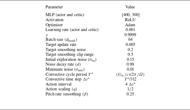

 Cp
 Cp=0
 αp=0∘
 αp(θ)
 ∘

 α¯p
 Δαeff
 αp=0∘

 Cp
 αp=0∘
 αp=6∘

 αp=0∘

 αp=6∘
 αp=0∘
 ∘
 αp=0∘
 αp=6∘
 CF,tot
 Cp
 CF,tot
 αeff
 Ueff/(ΩR)
 ∘
 ∘
 ∘
 ∘
 ∘
 ∘

 αp=0∘
 Cp
 θ
 αp
 θ
 ΔCp
 Cpopt−Cpαp=0∘
 θ=45∘
 135∘
 180∘
 225∘
 ∙
 ∙
 ∙
 αp
 ∙
 αp=0∘

 θ=45∘
 Q
 ψz
 −2×10⁻⁴
 −10−4
 0
 10−4
 2×10⁻⁴
 II∗
 |Cp,i|
 II∗
 Cp,i
 Cp,ω
 II
 θ=45∘
 Cp=0.076
 0.483

 θ=144∘
 Q
 ψz
 −2×10⁻⁴
 −10−4
 0
 10−4
 2×10⁻⁴
 II∗
 |Cp,i|
 II∗
 Cp,i
 Cp,ω
 II
 θ=144∘
 Cp=−0.028
 0.462

 θ=180∘
 Q
 ψz
 −2×10⁻⁴
 −10−4
 0
 10−4
 2×10⁻⁴
 II∗
 |Cp,i|
 II∗
 Cp,i
 Cp,ω
 II
 θ=180∘
 Cp=−0.341
 −0.058

 θ=315∘
 Q
 ψz
 −2×10⁻⁴
 −10−4
 0
 10−4
 2×10⁻⁴
 II∗
 |Cp,i|
 II∗
 Cp,i
 Cp,ω
 II
 θ=315∘
 Cp=−0.139
 0.144

 λ=1.9
 αp=6∘
 CFx
 CFy
 Cp

 Cp
 αp=6∘

 θ=102∘
 138∘
 165∘
 220∘

 Cp
 Cp,s
 Cp,pPPM
 Cp,pPPM

 αp=0∘

 45∘
 CF,tot
 Cp
 CF,tot
 αeff
 Ueff/(ΩR)
 0∘
 90∘
 90∘
 180∘
 180∘
 360∘

 ux
 uy
 ux=U∞
 uy=0
 …
 ΩR


