1. Introduction
Symmetry breaking was historically introduced in physics by Pierre Curie (Reference Curie1894), along with his well-known ‘Curie’s symmetry principle’ applied to electric and magnetic fields. It refers to any effects due to the change of one, or more, symmetry transformations which leave the system invariant. It therefore covers a large range of physical problems, including fluid mechanics where turbulence helicity appears, as the most well-known phenomenon affecting symmetries (Levich & Tsinober Reference Levich and Tsinober1983; Polifke Reference Polifke1990; Saint-Michel, Daviaud & Dubrulle Reference Saint-Michel, Daviaud and Dubrulle2014). Modifying the geometry (Davey & Salwen Reference Davey and Salwen1994), making the flow or boundaries rotate (Busse Reference Busse1984; Bourguet & Jacono Reference Bourguet and Jacono2013) or adding a peculiar mean flow (Bauerheim, Cazalens & Poinsot Reference Bauerheim, Cazalens and Poinsot2014a ), are other types of symmetry breaking recently investigated in fluid mechanics. When the order of the symmetry is reduced, specific behaviours may occur such as instabilities (Feng & Sethna Reference Feng and Sethna1989; Simonelli & Gollub Reference Simonelli and Gollub1989; Davey & Salwen Reference Davey and Salwen1994), splitting effects (Mazzei et al. Reference Mazzei, Gotzinger, Menezes, Zumofen, Benson and Sandoghdar2007; Kammerer et al. Reference Kammerer, Weigand, Curcic, Sproll, Vansteenkiste, Waeyenberge, Van Stoll, Woltersdorf, Back and Schuetz2011; Bauerheim et al. Reference Bauerheim, Salas, Nicoud and Poinsot2014e ) or even chaotic behaviours (Simonelli & Gollub Reference Simonelli and Gollub1989).
Recently, an increasing research effort is dedicated to the crucial role of symmetry breaking in unstable phenomena (Guckenheimer & Mahalov Reference Guckenheimer and Mahalov1992; Davey & Salwen Reference Davey and Salwen1994; Noiray, Bothien & Schuermans Reference Noiray, Bothien and Schuermans2011; Bourguet & Jacono Reference Bourguet and Jacono2013; Bauerheim et al. Reference Bauerheim, Salas, Nicoud and Poinsot2014e ). For instance, Bourguet & Jacono (Reference Bourguet and Jacono2013) revealed that the symmetry breaking induced by a rotating unconfined cylinder may impact the hydrodynamic instabilities, for example by suppressing the von Kármán street at high rotational speed. Similar effects on the flow topology were observed with a rotating confined cylinder (Camarri & Giannetti Reference Camarri and Giannetti2010), where the eccentricity of the rotating axis may enhance asymmetries (Prasad, Agrawal & Sharma Reference Prasad, Agrawal and Sharma2013). Such studies have spread to many fluid problems involving the growth of flow oscillations, such as surface waves generation (Feng & Sethna Reference Feng and Sethna1989; Simonelli & Gollub Reference Simonelli and Gollub1989), oscillations of rotating droplets (Busse Reference Busse1984; Cummings & Blackburn Reference Cummings and Blackburn1991) or hydrodynamic instabilities in elliptic pipes (Davey & Salwen Reference Davey and Salwen1994).
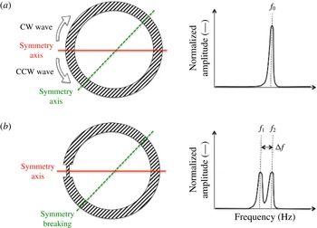
Sketch of a configuration with rotating symmetries ((a) infinite number of symmetry axis) and its associated spectrum (right). Two waves (clockwise (CW) and counter-clockwise (CCW)) can exist and have the same frequency
 $f_{0}$
: the mode is ‘degenerate’. When the rotating symmetry is broken ((b) only one symmetry axis remains), the degenerate mode at
 $f_{0}$
is split into two distinct waves with different yet close frequencies
 $f_{1}$
and
 $f_{2}$
.

In unstable systems containing rotating symmetries such as circular pipes or annular cavities, symmetry breaking appears with specificities by affecting preferably circumferential modes. When the rotating symmetry is perfect, these modes occur in doubly-degenerate pairs with two independent oscillations (a clockwise and a counter-clockwise waves) at the same frequency (figure 1 a). However, when the rotational symmetry is modified, degenerate pairs can split into two distinct modes with different yet close frequencies (figure 1 b). This phenomenon is known as the ‘splitting effect’ and usually makes the flow less stable (Guckenheimer & Mahalov Reference Guckenheimer and Mahalov1992; Davey & Salwen Reference Davey and Salwen1994; Bauerheim et al. Reference Bauerheim, Salas, Nicoud and Poinsot2014e ).
The authors of this paper have already analytically investigated the effect of a desired symmetry reduction to control azimuthal thermoacoustic instabilities in one annular cavity coupled with multiple flames (Bauerheim et al. Reference Bauerheim, Cazalens and Poinsot2014a ,Reference Bauerheim, Salas, Nicoud and Poinsot e ). These combustion instabilities remain a severe problem in the development of modern annular combustion chambers, where acoustic waves can couple with the unsteady heat release. It may produce large pressure and velocity oscillations leading to vibrations and structural damage (Krebs et al. Reference Krebs, Flohr, Prade and Hoffmann2002; Schuermans, Bellucci & Paschereit Reference Schuermans, Bellucci and Paschereit2003; Lieuwen & Yang Reference Lieuwen and Yang2005). In particular, azimuthal modes appearing in annular chambers raise many challenges because of their complexity. Over the last decade, they have been studied in symmetric configurations using both experiment (Moeck, Paul & Paschereit Reference Moeck, Paul and Paschereit2010; Bourgouin et al. Reference Bourgouin, Durox, Moeck, Schuller and Candel2013, Reference Bourgouin, Durox, Moeck, Schuller and Candel2014; Worth & Dawson Reference Worth and Dawson2013), simulation (Wolf et al. Reference Wolf, Staffelbach, Roux, Gicquel, Poinsot and Moureau2009, Reference Wolf, Staffelbach, Balakrishnan, Roux and Poinsot2010) and theory (Parmentier et al. Reference Parmentier, Salas, Wolf, Staffelbach, Nicoud and Poinsot2012; Bourgouin Reference Bourgouin2014). More recently, these studies have progressed to non-symmetric cases (Noiray et al. Reference Noiray, Bothien and Schuermans2011; Ghirardo & Juniper Reference Ghirardo and Juniper2013; Bauerheim et al. Reference Bauerheim, Cazalens and Poinsot2014a ; Dawson & Worth Reference Dawson and Worth2014). For instance, in a configuration containing one annular chamber, Bauerheim et al. (Reference Bauerheim, Cazalens and Poinsot2014a ,Reference Bauerheim, Salas, Nicoud and Poinsot e ) have identified theoretically a splitting effect due to either a distribution of different burners along the azimuthal direction (called geometrical symmetry breaking) or the addition of an azimuthal mean flow (denoted flow symmetry breaking), both of them leading to a less stable configuration. It suggests that perfectly symmetric gas turbines are less prone to combustion instabilities, which constitutes an idealized case out of reach for practical reasons such as manufacturing margins and tolerances.
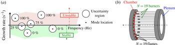
(a) Location in the frequency plane of the first six thermoacoustic modes in a typical combustor without uncertainties (single point, black symbols) and with uncertainties (each mode belongs to an admissible region of the frequency plane with an associated risk factor). (b) The annular configuration studied corresponds to two annular cavities coupled by
 $N=19$
burners and flames.

Consequently, the present paper focuses on symmetry breaking when it appears unintentionally, for example by taking into account random tolerances on the burner characteristics. This study will investigate the impact of such symmetry reductions on the stability of circumferential modes, which corresponds to a situation of practical and fundamental interests, since introducing uncertainty quantification for thermoacoustics has never been done before. Even though dealing with uncertainties in thermoacoustics cannot be fully studied today with expensive large eddy simulations (LES) or direct numerical simulations (DNS), it can be achieved with 3-D Helmholtz solvers or low-order models. These acoustic solvers characterize the stable/unstable modes in the frequency domain. An approximate linear wave equation for the small pressure perturbations
 $p^{\prime }(\boldsymbol{x},t)=\widehat{p}(\boldsymbol{x})\exp (-j{\it\omega}t)$
in reacting flows may be derived from the Navier–Stokes equations (Poinsot & Veynante Reference Poinsot and Veynante2005) and reads
 $$\begin{eqnarray}{\it\gamma}p_{0}\boldsymbol{{\rm\nabla}}\boldsymbol{\cdot }\left(\frac{1}{{\it\rho}_{0}}\boldsymbol{{\rm\nabla}}\widehat{p}\right)+{\it\omega}^{2}\widehat{p}=j{\it\omega}({\it\gamma}-1)\widehat{\dot{{\it\omega}_{T}}},\end{eqnarray}$$
where
 $\dot{{\it\omega}}_{T}^{\prime }(\boldsymbol{x},t)=\widehat{\dot{{\it\omega}_{T}}}(\boldsymbol{x})\exp (-j{\it\omega}t)$
is the unsteady heat release,
 $p_{0}$
and
 ${\it\rho}_{0}$
are the mean pressure and density,
 ${\it\gamma}$
is the heat capacity ratio and
 ${\it\omega}$
is the complex pulsation. In order to close the problem, the flame is often modelled as a purely acoustic element thanks to a
 $n{-}{\it\tau}$
model (Crocco Reference Crocco1952) or a matrix transfer (Polifke et al.
Reference Polifke, Poncet, Paschereit and Doebbeling2001), which essentially relates the unsteady heat release to acoustic quantities at reference locations. Equation (1.1) corresponds to a nonlinear eigenvalue problem which can be solved efficiently at reduced cost (Nicoud et al.
Reference Nicoud, Benoit, Sensiau and Poinsot2007).
The output of such a tool is typically a map of the thermoacoustic modes in the complex plane (see the black symbols, in figure 2
a). In this view, each mode is either stable or unstable, depending on the input parameters of the thermoacoustic analysis. Each mode corresponding to a positive imaginary frequency (positive growth rate,
 $\text{Im}({\it\omega})>0$
) is linearly unstable and must be controlled (e.g. by including acoustic dampers). The design process is made much more complex by the fact that the input parameters of the acoustic model described by (1.1) are uncertain. For example, the speed of sound
 $c_{0}$
, the boundary impedances and the flame forcing
 $\dot{{\it\omega}_{T}}(\boldsymbol{x},t)$
, are very sensitive to multiple physical parameters such as the flow regime, manufacturing tolerances, fuel changes and acoustic or heat losses, which are partly unknown (Duchaine et al.
Reference Duchaine, Boudy, Durox and Poinsot2011; Kedia, Altay & Ghoniem Reference Kedia, Altay and Ghoniem2011; Bauerheim et al.
Reference Bauerheim, Staffelbach, Worth, Dawson, Gicquel and Poinsot2014f
). As a consequence, each mode actually belongs to an uncertain region in the complex plane, as illustrated in figure 2(a). It is quantified by a risk factor defined as the probability for a mode to be unstable: this is a novel notion which renews the classical bi-modal stable/unstable view in thermoacoustics (Hoeijmakers et al.
Reference Hoeijmakers, Lopez Arteaga, Kornilov, Nijmeijer and de Goey2013). Even though our objective is to apply UQ in full 3-D Helmholtz solvers, it is first applied here using the ATACAMAC methodology (Parmentier et al.
Reference Parmentier, Salas, Wolf, Staffelbach, Nicoud and Poinsot2012; Bauerheim et al.
Reference Bauerheim, Parmentier, Salas, Nicoud and Poinsot2014d
) because (i) it is much more cost effective while retaining most of the characteristics of Helmholtz solvers, and (ii) partially analytical results are available for comparison (Bauerheim et al.
Reference Bauerheim, Parmentier, Salas, Nicoud and Poinsot2014d
).
In academic situations containing only one burner, the shape and size of these uncertain regions only depend on a few uncertain parameters such as the inlet air temperature, the amplitude and phase of the flame response and the boundary impedances (Duchaine et al.
Reference Duchaine, Boudy, Durox and Poinsot2011; Bauerheim et al.
Reference Bauerheim, Staffelbach, Worth, Dawson, Gicquel and Poinsot2014f
). The situation is more complex in realistic combustors used for power generation or aero-engines: they usually contain an annular chamber hosting several burners, typically from 15 to 24, and are prone to azimuthal combustion instabilities (Krebs et al.
Reference Krebs, Flohr, Prade and Hoffmann2002; Lieuwen & Yang Reference Lieuwen and Yang2005). In this case, the number of uncertain parameters may reach several tens since the gain and time delay of each flame are highly sensitive to manufacturing tolerances. This holds for the configuration retained in this paper, which is typical of a complex industrial combustor corresponding to an annular chamber connected to 19 burners fed by a common annular plenum (figure 2
b), leading to 38 uncertain parameters (only the 19 flame parameters
 $n$
and
 ${\it\tau}$
are retained here as random variables). The ‘curse of dimensionality’, well known in the UQ field, is thus becoming a problem when applying UQ to such systems. Indeed, dealing with more than 20 uncertain parameters is a tedious task, only tackled for linear or academic problems. Therefore, these large UQ problems require innovative approaches to reduce the dimensionality of the problem prior to applying standard techniques effective in low dimensions. Here, a novel approach for large UQ problems called ‘Active Subspace’ (Bauerheim et al.
Reference Bauerheim, Ndiaye, Constantine, Iaccarino, Moreau and Nicoud2014b
; Constantine, Dow & Wang Reference Constantine, Dow and Wang2014), will be used. This technique is similar to a proper orthogonal decomposition (POD, Kerschen et al.
Reference Kerschen, Golinval, Vakakis and Bergman2005; Rowley Reference Rowley2005) on the gradients of the output (here, the growth rate) to search for a new, and hopefully reduced, set of random variables better suited to the problem. Combined with partially analytical solutions, as it is for annular cavities coupled with multiple flames (Bauerheim et al.
Reference Bauerheim, Parmentier, Salas, Nicoud and Poinsot2014d
,Reference Bauerheim, Salas, Nicoud and Poinsot
e
), this UQ strategy allows also the identification of key parameters controlling the probabilistic problem. In other words, symmetry breaking effects induced by uncertainties can be unravelled and then quantified: this is the main objective of this paper.
First, the low-order ATACAMAC tool is presented in § 2 for two coupled annular cavities (figure 3) corresponding to an annular chamber connected to 19 burners fed by a common annular plenum. Before adding uncertainties, a perfect axisymmetric case is studied in § 2.3 to highlight a bifurcation separating two different regimes: (i) a weakly-coupled regime where acoustics is present only in the annular chamber and (ii) a strongly-coupled regime where both the annular chamber and the annular plenum affect the mode stability. Then, uncertainties are introduced and the UQ case is described along with the classical Monte Carlo method in § 3. This discussion illustrates that a novel approach to reduce the dimension of the probabilistic space is required. The present paper focuses on the active subspace approach presented in § 3.2. This novel UQ technique is applied on two annular cavities with 19 flames (figure 2 b) and containing 38 uncertain parameters to assess the risk factor associated with the first azimuthal mode in both the weakly and strongly-coupled regimes. Results show that only 3 active variables are required to fully describe the mode stability. This drastic reduction of dimensionality exemplifies the potential of this novel UQ technique. Moreover, the three active variables are shown to have a physical meaning related to symmetry-breaking effects. This symmetry reduction and associated destabilization effect appear due to the non-uniform pattern of the uncertainty distribution. It constitutes the main objective of this paper since stability is usually predicted on idealized configurations, resulting in a skewed risk estimation. Finally, a classical Monte Carlo technique is applied on this reduced 3-D space to fit algebraic models in § 4.2. These surrogate models are replayed thousands of times at low cost to predict the probability density function (PDF) of the growth rate and to compute the associated risk factor. These models allow the extraction and quantification of the symmetry-breaking effects on the growth-rate PDF. This risk factor estimation is then compared with the one obtained by a full Monte Carlo analysis showing a good agreement with errors below 5 % for both the weakly and strongly-coupled regimes.
2. Thermoacoustics in two coupled annular cavities
2.1. Mathematical framework
In the last decade, theoretical approaches for thermoacoustics in annular chambers have been applied on simplified annular configurations (Noiray et al.
Reference Noiray, Bothien and Schuermans2011; Parmentier et al.
Reference Parmentier, Salas, Wolf, Staffelbach, Nicoud and Poinsot2012) to complement 3-D Helmholtz simulations (Pankiewitz & Sattelmayer Reference Pankiewitz and Sattelmayer2003; Campa et al.
Reference Campa, Camporeale, Guaus, Favier, Bargiacchi, Bottaro, Cosatto and Mori2011) and LES (Wolf et al.
Reference Wolf, Staffelbach, Gicquel, Muller and Poinsot2012). Recently, the analytical ATACAMAC tool (analytical tool to analyse and control azimuthal mode in annular chambers) has been developed to handle configurations where one annular chamber connects
 $N$
burners (Parmentier et al.
Reference Parmentier, Salas, Wolf, Staffelbach, Nicoud and Poinsot2012; Bauerheim et al.
Reference Bauerheim, Salas, Nicoud and Poinsot2014e
). Note that a complete analytical solution can be derived for axisymmetric and non-axisymmetric cases (Bauerheim et al.
Reference Bauerheim, Cazalens and Poinsot2014a
,Reference Bauerheim, Salas, Nicoud and Poinsot
e
). This tool has been extended to more complex geometries with two annular cavities (Bauerheim et al.
Reference Bauerheim, Cazalens and Poinsot2014a
): one annular chamber is fed by
 $N$
burners connected to a common annular plenum, as illustrated in figure 3. In such systems, the two annular cavities can couple and may impact the symmetry-breaking mechanisms. However, no analytical solution is available today for this configuration when the burners are different (i.e. for asymmetric cases).
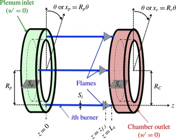
Sketch of a configuration where an annular chamber (right) is fed by
 $N$
burners connected to a common annular plenum (left). The
 $i$
th flame is located in the burner at the location
 $z_{f,i}={\it\alpha}L_{i}$
and is modelled using a FTF with two parameters: an amplitude
 $n_{i}$
and a time delay
 ${\it\tau}_{i}$
.

This paper focuses on such a configuration where an annular chamber connects
 $N=19$
burners fed by a common annular plenum (figure 3). The two annular cavities are characterized by their half-perimeters
 $L_{p}={\rm\pi}R_{p}$
and
 $L_{c}={\rm\pi}R_{c}$
and cross-sections
 $S_{p}$
and
 $S_{c}$
. All fluctuating quantities
 $a^{\prime }(x,t)$
such as the pressure
 $p^{\prime }$
, the axial velocity
 $w^{\prime }$
and the azimuthal velocity
 $u^{\prime }$
, are assumed harmonic:
 $a^{\prime }(x,t)=\hat{a}(x)\text{e}^{-j{\it\omega}t}$
. In these two cavities, the azimuthal position is given by the angle
 ${\it\theta}$
associated with a curvilinear abscissa
 $x_{p}=R_{p}{\it\theta}$
in the plenum and
 $x_{c}=R_{c}{\it\theta}$
in the chamber. Null axial acoustic velocity
 ${\hat{w}}=0$
is assumed in both cavities leading to pure azimuthal modes: the acoustic velocity has only one non-null component
 $\hat{u}$
which depends only on
 ${\it\theta}$
in the annular cavities. Thus, at one azimuthal location,
 ${\it\theta}$
corresponds one acoustic state
 $\mathit{X}_{{\it\theta}}=[\hat{p}_{p}({\it\theta}),\hat{u} _{p}({\it\theta}),\hat{p}_{c}({\it\theta}),\hat{u} _{c}({\it\theta})]^{\text{T}}$
.
In the
 $N$
burners, modelled by 1-D tubes along the
 $z$
-axis, the axial acoustic fluctuations
 ${\hat{w}}(z)$
can be non-null and excite the flames. They are modelled here by a flame transfer function (FTF, Crocco & Cheng Reference Crocco and Cheng1956) which relates the unsteady heat release
 $\widehat{\dot{{\it\omega}_{T}}}$
to the acoustic velocity in the
 $i$
th burner
 $\widehat{w}(z_{f,i})$
:
 $$\begin{eqnarray}\frac{{\it\gamma}_{u}-1}{{\it\gamma}_{u}p_{0}}\widehat{\dot{{\it\omega}_{T}}}=S_{i}n_{i}\text{e}^{j{\it\omega}{\it\tau}_{i}}\widehat{w}(z_{f,i}),\end{eqnarray}$$
where
 ${\it\gamma}_{u}$
is the unburnt heat capacity ratio,
 $p_{0}$
is the mean pressure,
 $S_{i}$
is the burner section,
 $n_{i}$
is the FTF amplitude and
 ${\it\tau}_{i}$
its time delay and
 ${\it\omega}$
is the pulsation of the acoustic mode. The present flame model is based on the longitudinal velocity fluctuations
 ${\hat{w}}$
, since the azimuthal modes act like a clock, modulating the mass flow rate in the burner which feeds the flame (O’Connor & Lieuwen Reference O’Connor and Lieuwen2014). This is the main mechanism leading to combustion instabilities, at least for flames not located at a pressure node.
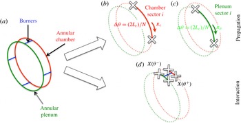
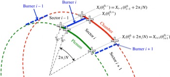
(a) ANR methodology where the annular combustor is split into
 $N$
sectors. Each sector is then split into a propagation part (b,c) either in the annular plenum or chamber and an interaction part ((d) between annular cavities and burners). Unknown at white cross locations are the acoustic pressure and velocity.

The annular network reduction (ANR) methodology detailed in Bauerheim et al. (Reference Bauerheim, Parmentier, Salas, Nicoud and Poinsot2014d
) is applied on this geometry. It splits the annular configuration into
 $N=19$
sectors (figure 4). Then, for each individual sector, the acoustic problem may be split into two parts:
-
(i) Propagation in the annular cavities (plenum or chamber): the plenum and the chamber can be treated separately, the acoustic state
 $\mathit{X}_{i}({\it\theta})$
at one location
${\it\theta}$
in the
$i$
th sector being related to the acoustic quantity at the location
${\it\theta}+{\rm\Delta}{\it\theta}$
by a
$4\times 4$
rotation matrix
$\unicode[STIX]{x1D64D}_{i}({\rm\Delta}{\it\theta})$
(2.2)where
$$\begin{eqnarray}\mathit{X}_{i}({\it\theta}+{\rm\Delta}{\it\theta})=\unicode[STIX]{x1D64D}_{i}({\rm\Delta}{\it\theta})\mathit{X}_{i}({\it\theta})\quad \text{where }\unicode[STIX]{x1D64D}_{i}({\rm\Delta}{\it\theta})=\left[\begin{array}{@{}cc@{}}\unicode[STIX]{x1D64D}(k_{u}R_{p}{\rm\Delta}{\it\theta}) & \begin{array}{@{}cc@{}}0 & 0\\ 0 & 0\end{array}\\ \begin{array}{@{}cc@{}}0 & 0\\ 0 & 0\end{array} & \unicode[STIX]{x1D64D}(kR_{c}{\rm\Delta}{\it\theta})\end{array}\right],\end{eqnarray}$$
$\unicode[STIX]{x1D64D}(x)=\left[\begin{smallmatrix}\cos (x) & -\sin (x)\\ \sin (x) & \cos (x)\end{smallmatrix}\right]$
is the
$2\times 2$
rotation matrix of angle
$x$
,
$k={\it\omega}/c^{0}$
is the acoustic wavenumber in the burnt gases (annular chamber) and
$k_{u}={\it\omega}/c_{u}^{0}$
is the acoustic wavenumber in the unburnt gases (annular plenum). This expression exemplifies that the acoustic quantities in the plenum are not correlated to the ones in the annular chamber when only acoustic propagation occurs.
-
(ii) Interactions which couple the annular plenum and the annular chamber via the burners and the flames: acoustic pressure and velocity before the junction (
${\it\theta}^{-}$
) are linked to the acoustic quantities after the junction (
${\it\theta}^{+}$
) by a
$4\times 4$
matrix
$\unicode[STIX]{x1D64F}_{i}$
. This matrix depends on four coupling parameters, initially introduced for longitudinal cases with passive flames by Schuller et al. (Reference Schuller, Durox, Palies and Candel2012), and extended for annular configurations with active flames by Bauerheim et al. (Reference Bauerheim, Parmentier, Salas, Nicoud and Poinsot2014d
):
${\it\Gamma}_{i,1}$
corresponds to the plenum/burner interaction whereas
${\it\Gamma}_{i,4}$
is associated with the chamber/burner coupling.
${\it\Gamma}_{i,2}$
and
${\it\Gamma}_{i,3}$
are cross-interactions between the plenum and the chamber. The matrix
$\unicode[STIX]{x1D64F}_{i}$
is obtained from jump conditions (Bauerheim et al.
Reference Bauerheim, Parmentier, Salas, Nicoud and Poinsot2014d
) at null Mach number (Dowling Reference Dowling1995; Bauerheim, Nicoud & Poinsot Reference Bauerheim, Nicoud and Poinsot2014c
). The interaction matrix
$\unicode[STIX]{x1D64F}_{i}$
reads (2.3)where
$$\begin{eqnarray}X({\it\theta}^{+})=\unicode[STIX]{x1D64F}_{i}X({\it\theta}^{-})\quad \text{where }\unicode[STIX]{x1D64F}_{i}=\unicode[STIX]{x1D644}_{d}+2\left[\begin{array}{@{}cccc@{}}0 & 0 & 0 & 0\\ {\it\Gamma}_{i,1} & 0 & {\it\Gamma}_{i,2} & 0\\ 0 & 0 & 0 & 0\\ {\it\Gamma}_{i,3} & 0 & {\it\Gamma}_{i,4} & 0\end{array}\right],\end{eqnarray}$$
$\unicode[STIX]{x1D644}_{d}$
is the identity matrix and the coefficients
${\it\Gamma}_{i,k}$
,
$k=1$
to 4 are with the flame parameter(2.4)
$$\begin{eqnarray}\displaystyle & \displaystyle {\it\Gamma}_{i,1}=-\frac{1}{2}\frac{S_{i}}{S_{p}}\frac{\cos (k(1-{\it\alpha})L_{i})\cos (k_{u}{\it\alpha}L_{i})-\mathbb{F}\sin (k(1-{\it\alpha})L_{i})\sin (k_{u}{\it\alpha}L_{i})}{\cos (k(1-{\it\alpha})L_{i})\sin (k_{u}{\it\alpha}L_{i})+\mathbb{F}\sin (k(1-{\it\alpha})L_{i})\cos (k_{u}{\it\alpha}L_{i})}, & \displaystyle\end{eqnarray}$$
(2.5)
$$\begin{eqnarray}\displaystyle & \displaystyle {\it\Gamma}_{i,2}=\frac{1}{2}\frac{S_{i}}{S_{p}}\frac{1}{\cos (k(1-{\it\alpha})L_{i})\sin (k_{u}{\it\alpha}L_{i})+\mathbb{F}\sin (k(1-{\it\alpha})L_{i})\cos (k_{u}{\it\alpha}L_{i})}, & \displaystyle\end{eqnarray}$$
(2.6)
$$\begin{eqnarray}\displaystyle & \displaystyle {\it\Gamma}_{i,3}=\frac{1}{2}\frac{S_{i}}{S_{c}}\frac{\mathbb{F}}{\cos (k(1-{\it\alpha})L_{i})\sin (k_{u}{\it\alpha}L_{i})+\mathbb{F}\sin (k(1-{\it\alpha})L_{i})\cos (k_{u}{\it\alpha}L_{i})}, & \displaystyle\end{eqnarray}$$
(2.7)
$$\begin{eqnarray}\displaystyle & \displaystyle {\it\Gamma}_{i,4}=-\frac{1}{2}\frac{S_{i}}{S_{c}}\frac{\mathbb{F}\cos (k(1-{\it\alpha})L_{i})\cos (k_{u}{\it\alpha}L_{i})-\sin (k(1-{\it\alpha})L_{i})\sin (k_{u}{\it\alpha}L_{i})}{\cos (k(1-{\it\alpha})L_{i})\sin (k_{u}{\it\alpha}L_{i})+\mathbb{F}\sin (k(1-{\it\alpha})L_{i})\cos (k_{u}{\it\alpha}L_{i})}, & \displaystyle\end{eqnarray}$$
$\mathbb{F}$
(2.8)One should note that if the acoustic mode does not interact with the flames and the burners, then all coupling parameters are zero and therefore this interaction matrix reduces to
$$\begin{eqnarray}\mathbb{F}=\frac{{\it\rho}^{0}c^{0}}{{\it\rho}_{u}^{0}c_{u}^{0}}(1+n\text{e}^{j{\it\omega}{\it\tau}}).\end{eqnarray}$$
$\unicode[STIX]{x1D64F}_{i}=\unicode[STIX]{x1D644}_{d}$
. Note also that all coupling terms relate a velocity in one cavity to pressure in both cavities, for instance
$-j{\it\rho}^{0}c^{0}\hat{u} _{i+1,c}=-j{\it\rho}^{0}c^{0}\hat{u} _{i,c}+2{\it\Gamma}_{i,3}\hat{p}_{i,p}+2{\it\Gamma}_{i,4}\hat{p}_{i,c}$
. Consequently, whatever the value of the coupling parameters, there is no interaction when a burner is located at a pressure node.






2.2. Construction and resolution of the dispersion relation
Using the propagation (2.2) and interaction (2.3) matrices, the
 $4\times 4$
matrix associated with the complete
 $i$
th sector (interaction plus propagation, where the interaction with the
 $i$
th burner takes place at
 ${\it\theta}={\it\theta}_{i}^{0}$
, and then the acoustics propagates all along the
 $i$
th sector corresponding to
 ${\rm\Delta}{\it\theta}=2{\rm\pi}/N$
, as illustrated in figure 5) is then equal to
 $\unicode[STIX]{x1D64D}_{i}\unicode[STIX]{x1D64F}_{i}$
because
 $$\begin{eqnarray}\mathit{X}_{i}({\it\theta}_{i}^{0}+2{\rm\pi}/N)=\unicode[STIX]{x1D64D}_{i}\mathit{X}_{i}({\it\theta}_{i}^{0,+})=\unicode[STIX]{x1D64D}_{i}\unicode[STIX]{x1D64F}_{i}\mathit{X}_{i}({\it\theta}_{i}^{0,-}).\end{eqnarray}$$
Since the quantities between neighbouring sectors are equivalent (i.e.
 $\mathit{X}_{i}({\it\theta}_{i}^{0,-})=\mathit{X}_{i-1}({\it\theta}_{i}^{0}+2{\rm\pi}/N)$
) and using the periodicity condition (
 $\mathit{X}_{N+1}({\it\theta}_{N+1}^{0})=\mathit{X}_{1}({\it\theta}_{1}^{0})$
), it yields
 $$\begin{eqnarray}\mathit{X}_{1}({\it\theta}_{1}^{0})=\left(\mathop{\prod }_{k=N}^{1}\unicode[STIX]{x1D64D}_{i}\unicode[STIX]{x1D64F}_{i}\right)\mathit{X}_{1}({\it\theta}_{1}^{0}).\end{eqnarray}$$
This eigenvalue problem has non-trivial solutions if and only if its determinant is null:
 $$\begin{eqnarray}\det \left(\mathop{\prod }_{k=N}^{1}\unicode[STIX]{x1D64D}_{i}\unicode[STIX]{x1D64F}_{i}-\unicode[STIX]{x1D644}_{d}\right)=0.\end{eqnarray}$$
Acoustic quantities
 $\mathit{X}_{i}$
in the
 $i$
th sector of the annular combustor at several azimuthal locations
 ${\it\theta}$
.

This dispersion relation can be solved to obtain the complex angular frequency
 ${\it\omega}$
without knowing the mode structure characterized by the eigenvector
 $\mathit{X}_{1}({\it\theta}_{1}^{0})$
. Bauerheim et al. (Reference Bauerheim, Parmentier, Salas, Nicoud and Poinsot2014d
) proposed two methodologies to solve this equation depending on the coupled regime, i.e. if one or both cavities drive the azimuthal mode:
-
(i) Weakly-coupled modes. When acoustics is present in only one annular cavity, Bauerheim et al. (Reference Bauerheim, Parmentier, Salas, Nicoud and Poinsot2014d ) have derived an analytical expression of the complex frequency for the axisymmetric case. It is based on a small perturbation assumption, which allows a Taylor expansion of the dispersion relation. In this case, any azimuthal modes of the chamber can be studied by replacing the annular plenum by an impedance
$Z=0$
at the upstream end of the burners (corresponding to a pressure node imposed by the large plenum). In non-symmetric cases (where burners or flames are different), it can be inferred that weakly coupled modes can still be investigated by removing the plenum. In this case, Bauerheim et al. (Reference Bauerheim, Salas, Nicoud and Poinsot2014e
) have shown that the frequency
$f_{p}$
of the
$p$
th circumferential mode of the chamber is controlled by two parameters. Indeed, they obtained the following expression for the frequency (2.12)where
$$\begin{eqnarray}f_{p}=\frac{pc^{0}}{2L_{c}}-\frac{c^{0}}{4{\rm\pi}L_{c}}({\it\Sigma}_{0}\pm \mathscr{S}_{0}),\end{eqnarray}$$
(2.13)and
$$\begin{eqnarray}{\it\Sigma}_{0}=\mathop{\sum }_{i=1}^{N}{\it\Gamma}_{i}^{0}=\widehat{{\it\Gamma}^{0}}(0),\end{eqnarray}$$
(2.14)In these expressions,
$$\begin{eqnarray}\mathscr{S}_{0}=\sqrt{\mathop{\sum }_{i,l=1}^{N}{\it\Gamma}_{i}^{0}{\it\Gamma}_{l}^{0}\cos \left(\frac{4p{\rm\pi}}{N}[i-l]\right)}=\sqrt{\widehat{{\it\Gamma}^{0}}(2p)\widehat{{\it\Gamma}^{0}}(-2p)}.\end{eqnarray}$$
${\it\Gamma}_{i}^{0}$
is the coupling parameter between the
$i$
th burner and the annular chamber (i.e.
${\it\Gamma}_{i,4}$
of (2.7)) evaluated at the initial frequency
$f_{0}=pc^{0}/2L_{c}$
. Thus
${\it\Sigma}_{0}$
and
$\mathscr{S}_{0}$
can be interpreted as the coupling strength due to the mean flame effect, and the splitting strength due to the asymmetry (different burners). These two parameters can be recast using the Fourier coefficients
$\widehat{{\it\Gamma}}(k)=\sum _{i=1}^{N}{\it\Gamma}_{i}\text{e}^{-j2{\rm\pi}k\text{i}/N}$
of the collection of coupling parameters
$\{{\it\Gamma}^{0}\}_{i=1,\ldots ,N}$
, viewed as a periodic discrete complex signal along the azimuthal chamber. This analytical solution has been validated against 3-D Helmholtz simulations in academic combustors with
$N=3$
and
$N=24$
burners (Bauerheim et al.
Reference Bauerheim, Salas, Nicoud and Poinsot2014e
). This is valid if the small perturbation assumption
$\Vert {\it\Sigma}_{0}\Vert \ll 1$
is satisfied: this regime is called ‘weakly coupled’.
-
(ii) Strongly-coupled modes. When the coupling parameters increase (i.e. when flames become more sensitive to acoustics), a bifurcation can occur. This corresponds to a strong coupling between the two annular cavities, which can change the stability of the whole system (Bauerheim et al. Reference Bauerheim, Parmentier, Salas, Nicoud and Poinsot2014d ). Acoustic activity is then present in both annular cavities with a phase-lag between the fluctuating pressure in the chamber and in the plenum. This regime is called strongly coupled and cannot be tackled analytically: one objective of this paper is therefore to use the active subspace approach to determine key parameters controlling this type of mode. Indeed, even if no analytical solution exists today, the dispersion relation (2.11) can be solved numerically using a Newton–Raphson algorithm as proposed by Parmentier et al. (Reference Parmentier, Salas, Wolf, Staffelbach, Nicoud and Poinsot2012). Bauerheim et al. (Reference Bauerheim, Parmentier, Salas, Nicoud and Poinsot2014d ) has validated this approach using a 3-D Helmholtz solver revealing a bifurcation mechanism between the weakly and the strongly-coupled regimes (§ 2.3).





2.3. Application to a deterministic case with
$N=19$
burners

The mathematical framework described previously is applied here on a combustor equipped with two annular cavities and
 $N=19$
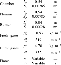
burners. This section considers a deterministic axisymmetric case to classify plenum/chamber and weakly/strongly coupled modes of this configuration, where geometrical and mean-flow characteristics are known perfectly (no uncertainty) and given in table 1. UQ and symmetry breaking will be investigated in the next sections.
Parameters used for numerical applications corresponding to a configuration equipped with two annular cavities and
 $N=19$
burners. They correspond to a typical aircraft engine.

The annular configuration is perfectly axisymmetric with identical burners and flames so that all flame parameters
 $(n_{i},{\it\tau}_{i})$
, coupling parameters
 ${\it\Gamma}_{i}$
and matrices
 $\unicode[STIX]{x1D64D}_{i}$
or
 $\unicode[STIX]{x1D64F}_{i}$
are exactly the same (the subscript
 $i$
can be omitted in this section). Parameters of the FTF are varied to produce stability maps and unveil mode trajectories as well as coupling between cavities (Bauerheim et al.
Reference Bauerheim, Parmentier, Salas, Nicoud and Poinsot2014d
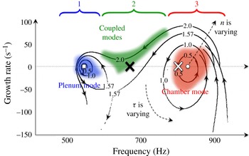
). Figure 6 highlights three different mode types: weakly-coupled chamber modes (3rd zone), weakly-coupled plenum modes (1st zone) and strongly coupled modes (2nd zone). This paper will focus on the first azimuthal mode of the combustion chamber (2nd and 3rd zones). Two operating points are identified using this stability map of the axisymmetric case provided in figure 6. These operating points characterize the values for
 $n$
and
 ${\it\tau}$
of the
 $N$
identical flames:
-
(i) Weakly-coupled chamber mode with
$n=0.5$
and
${\it\tau}=0.635~\text{ms}$
(white cross in figure 6). -
(ii) Strongly-coupled mode with
$n=1.75$
and
${\it\tau}=0.735~\text{ms}$
(black cross in figure 6).


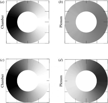
Figure 7 shows the associated structure of the acoustic mode obtained in the annular plenum and the annular chamber by ATACAMAC for the two operating points: the weakly (white cross in figure 6) and strongly (black cross in figure 6) coupled cases. This mode structure is obtained by injecting the known eigenfrequency into the eigenproblem (2.10) and numerically computing the associated eigenvector
 $\mathit{X}_{1}({\it\theta}_{1}^{0})$
. This eigenvector corresponds to the acoustic state in the plenum and in the chamber at one particular location in the first sector. This state is then propagated using the propagation and interaction matrices (2.2) and (2.3) to generate the whole mode structure displayed in figure 7. It shows that changing the flame responses (i.e. changing the FTF) modifies the coupling between the two annular cavities. In particular, the ratio of the acoustic pressures in the plenum and in the chamber is
 $27\,\%$
in the weakly-coupled regime and
 $70\,\%$
in the strongly-coupled regime. The latter case, where the acoustic pressure is present in the two cavities, cannot be investigated analytically since the low coupling factors assumption (
 $\Vert {\it\Sigma}_{0}\Vert \ll 1$
) is not valid. However, combining the numerical resolution of the analytical dispersion relation provided by ATACAMAC with a UQ approach can unveil coupling mechanism effects on symmetry breaking, and therefore on the stability of the system. In the following sections, the weakly and strongly-coupled cases will be studied using the numerical resolution of the dispersion relation (2.11).
Frequencies and growth rates of modes computed numerically for identical flames with FTF deterministic inputs:
 $n=0.5$
, 1.0, 1.57 and 2.0;
 ${\it\tau}=0{-}0.55~\text{ms}$
. Plenum (▫) and chamber (○) modes with passive flames are also displayed. Three different mode types are identified: weakly coupled chamber modes (3rd zone), weakly-coupled plenum modes (1st zone) and strongly-coupled modes (2nd zone). Only two operating points are chosen for UQ which correspond to marginally stable weakly (white cross) or strongly (black cross) coupled chamber modes. UQ results associated with weakly and strongly-coupled modes are shown in appendix A.

Structure of the acoustic mode (acoustic pressure
 $p^{\prime }=\Vert \hat{p}\Vert \cos (\arg (\hat{p}))$
) in the annular plenum and the annular chamber obtained by ATACAMAC for the two regimes: weakly (
 $\bar{n}=0.5$
,
 $\bar{{\it\tau}}=0.635$
ms) (a,b) and strongly (
 $\bar{n}=1.75$
,
 $\bar{{\it\tau}}=0.735$
ms) (c,d) coupled cases.

3. The active subspace approach for large UQ problems
3.1. Description of the UQ cases
The classical deterministic approach performed in § 2.3 is useful to classify modes in absence of any uncertainty (figure 8
b), as well as to identify weakly and strongly-coupled modes (figure 6). However, probabilistic methods are also required to fully describe the stability of acoustic modes by taking into account uncertainties. In this paper, FTF parameters
 $n_{i}$
and
 ${\it\tau}_{i}$
are assumed to be the only source of uncertainty leading to 38 random variables. This can be considered as a large nonlinear UQ problem. Of course, it is necessary to specify how these uncertainties are defined and distributed along the azimuthal direction. In this study, all flames have the same PDF for
 $n_{i}$
and
 ${\it\tau}_{i}$
(figure 8
c). These PDF are characterized by a mean value (
 $\bar{n}$
and
 $\bar{{\it\tau}}$
) and standard deviations (
 ${\it\sigma}_{n}$
and
 ${\it\sigma}_{{\it\tau}}$
), given in table 2. Mean values are determined according to the operating point chosen. Two different cases are considered: the first one called the ‘Wcase’ in the weakly-coupled regime (white cross in figure 6) and the second one called ‘Scase’, which corresponds to a strongly-coupled regime (black cross in figure 6). Standard deviations are chosen as 5 % (for
 ${\it\tau}$
) and
 $10\,\%$
(for
 $n$
) of their mean values according to experimental observations from different well-known groups (Cambridge, Ecole Centrale Paris, IMF Toulouse), and numerical sensitivity analysis (Duchaine et al.
Reference Duchaine, Boudy, Durox and Poinsot2011; Bauerheim et al.
Reference Bauerheim, Staffelbach, Worth, Dawson, Gicquel and Poinsot2014f
). In the absence of additional information about the distribution function of these parameters, uniform PDFs have been used for the sake of simplicity and their finite range. This assumption has obviously an impact on the results but not on the robustness and feasibility of the UQ strategy proposed here. Finally, this corresponds to cases where uncertainties are due to random tolerance margins: the 19 burners are picked up from a set of burners produced with the same tool but exhibiting random changes from one burner to the other. Note however that these uncertainties are fixed in time, which correspond to manufacturing tolerances, compared to uncertainties varying in time, for instance because of a background noise induced by turbulence. As suggested by Noiray et al. (Reference Noiray, Bothien and Schuermans2011), it would lead to a parametric noise (Lieuwen & Banaszuk Reference Lieuwen and Banaszuk2005) affecting the growth rate and limit cycle (Clavin, Kim & Williams Reference Clavin, Kim and Williams1994; Noiray et al.
Reference Noiray, Bothien and Schuermans2011). Nevertheless, Noiray et al. only consider a parametric noise constant in the azimuthal direction, while turbulence should affect all flames differently. In such a case, a splitting effect due to turbulence would appear as for the manufacturing tolerances but is not discussed in the present study for the sake of simplicity.
Present (c) and past (a,b) studies on azimuthal modes. The current study introduces UQ in thermoacoustics with the same PDF for all flames. Of course, random values can be different from one burner to another. It simulates the effect of tolerance margins on burner characteristics.

Summary of the two UQ cases investigated in this paper. Note that
 $\Vert {\it\Sigma}_{0}\Vert$
scales with the mean FTF amplitude like
 $\Vert {\it\Sigma}_{0}\Vert \propto 1+\bar{n}$
.

3.2. The classical Monte Carlo analysis
This section briefly presents the classical Monte Carlo method used for uncertainty quantification before focusing on the active subspace approach in § 3.3. The question addressed in the following is to find a robust cost-effective method to compute the probability density function, or at least the first statistical moments (mean value, standard deviation etc.), of an output
 $Y$
knowing the PDF of a number
 $D$
of inputs
 $h_{i=1,\ldots ,D}$
:
 $h=(n_{i},{\it\tau}_{i})_{i=1,\ldots ,N}$
so that
 $D=38$
for
 $N=19$
burners. This problem is known as the forward uncertainty-propagation problem (Chantrasmi & Iaccarino Reference Chantrasmi and Iaccarino2012) where the output is viewed as the result of a ‘black box’, which can be an experiment, a low-order model or a numerical solver, characterized by an unknown function
 $g$
:
 $$\begin{eqnarray}Y=g(h_{i})\quad \text{where PDFs of }h_{i}\text{ are known.}\end{eqnarray}$$
In this paper,
 $Y$
corresponds to the imaginary part of the complex frequency
 $\text{Im}(f)$
, denoted
 $f_{Im}$
in this work, and the
 $h_{i}$
are the 38 independent parameters
 $n_{i}$
and
 ${\it\tau}_{i}$
of the 19 burners. From the PDF of this growth rate, the probability of the acoustic mode to be unstable can be computed and is called the ‘risk factor’:
 $0\,\%$
indicates that the mode is perfectly stable,
 $100\,\%$
that the mode is always unstable.
 $$\begin{eqnarray}\text{RF}\,(\%)=100\int _{0}^{\infty }\text{PDF}(f_{Im})\,\text{d}f_{Im},\end{eqnarray}$$
knowing that
 $\int _{-\infty }^{\infty }\text{PDF}(f_{Im})\,\text{d}f_{Im}=1$
from the PDF definition.
To compute the PDF of the growth rate, necessary to construct the risk factor, several UQ approaches can be used. First, in this study, a Monte Carlo analysis has been performed. This well-known brute force method relies on repeated evaluations of the function
 $g$
using a random sampling of the inputs
 $h_{i}$
.
 $M$
random values of
 $h_{i}$
are chosen with respect to their known PDFs. The function
 $g$
is evaluated
 $M$
times to provide
 $M$
output values
 $f_{Im}^{k=1,\ldots ,M}$
. This method always converges but suffers from a slow convergence speed (
 $v(M,D)=1/\sqrt{M}$
) which can become prohibitive if the function
 $g$
is expensive to evaluate (Kaarnioja Reference Kaarnioja2013). Note that the convergence rate
 $v(M,D)$
, which quantifies the error reduction with the number of samples,
 $M$
, is independent of the dimension
 $D$
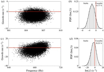
, which yields a robust method in high dimension. This method is used in this work, where thousands of ATACAMAC simulations are performed to produce a risk-factor estimation considered as a reference value. Two examples of such Monte Carlo analysis are displayed for the weakly and strongly-coupled modes in the appendix A. However, to apply UQ to more expensive tools such as 3-D Helmholtz solvers, other strategies with faster convergence speed are required.
Other UQ techniques have been developed to improve the slow convergence speed of the Monte Carlo analysis, such as quasi-Monte Carlo, stochastic collocation, sparse grid etc. (Nobile, Tempone & Webster Reference Nobile, Tempone and Webster2008; Kaarnioja Reference Kaarnioja2013), but usually lead to robustness problems, in particular for non-smooth function
 $g$
. Moreover, this convergence speed is often increased only in low dimensions. For instance, the quasi-Monte Carlo technique leads to a convergence speed proportional to
 $v(M,D)=\ln (M)^{D}/M$
, where
 $D$
is the input space dimension (Kaarnioja Reference Kaarnioja2013), which is theoretically faster than a classical Monte Carlo technique but only for low dimensions (typically
 $D<5$
).
In this paper, a novel UQ approach called ‘active subspace’ (Constantine et al.
Reference Constantine, Dow and Wang2014; Constantine Reference Constantine2015) is used to reduce the dimension of the parameter space from
 $D=38$
to just a few. This is desirable since working with 38 dimensions is too expensive even for 3-D Helmholtz solvers: only low-order models such as ATACAMAC can be applied directly on the full parameter space, for example with Monte Carlo techniques. The active subspace method provides a solution around this issue. In this context, ATACAMAC is used to compared results using the dimension reduction with a Monte Carlo analysis on the full parameter space, only possible using such a cost-effective tool. This method requires gradient evaluations to detect which directions in the parameter space lead to strong variations of the growth rate. Other directions leading to flat response surface are not useful for describing the dynamics of the system and can be disregarded. It leads to a UQ analysis which can be performed on a many fewer variables. Consequently, this method can therefore be viewed as a preprocessing tool acting on the dimension
 $D$
directly, before applying other classical UQ methods, and is described in the next section.
3.3. The active subspace approach
The poor effectiveness of standard UQ methods in high dimensions calls for the introduction of new UQ techniques. In this paper, the active subspace approach (Bauerheim et al. Reference Bauerheim, Ndiaye, Constantine, Iaccarino, Moreau and Nicoud2014b ; Constantine et al. Reference Constantine, Dow and Wang2014) is applied on the case presented in § 3.1. This technique is similar to a proper orthogonal decomposition (POD) but on the gradients of the random output (here, the growth rate).
First, the gradients of the growth rate
 $f_{Im}(h)$
with respect to the input parameters
 $h=\{n_{i},{\it\tau}_{i}\}_{i=1,\ldots ,N}$
, denoted
 $\boldsymbol{{\rm\nabla}}f_{Im}(h^{k})=\boldsymbol{{\rm\nabla}}_{h}^{k}f_{Im}$
for the
 $k$
th sample, must be computed. They can be obtained analytically in some cases, by an adjoint method (Juniper et al.
Reference Juniper, Magri, Bauerheim and Nicoud2015), or more generally by finite differences.
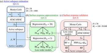
UQ strategy applied to an annular combustor with 38 uncertain parameters. First, the active subspace approach allows the reduction of the dimension from 38 to only 3 parameters (a). Then, surface responses are analysed using low-order models on both the full (FL, FQ and FC models) and reduced (RL, RQ and RC models) probabilistic spaces (b). Finally, the risk factor (RF) is computed using the low-order models and validated against ATACAMAC results on 10 000 samples (c).

Using
 $M$
evaluations of the gradient
 $\boldsymbol{{\rm\nabla}}_{h}^{k}f_{Im}$
, the uncentred covariance matrix
 $\unicode[STIX]{x1D63E}$
of the gradient vector can be obtained
 $$\begin{eqnarray}\unicode[STIX]{x1D63E}=\mathbb{E}[(\boldsymbol{{\rm\nabla}}_{h}^{k}f_{Im})(\boldsymbol{{\rm\nabla}}_{h}^{k}f_{Im})^{\text{T}}]\simeq \frac{1}{M}\mathop{\sum }_{k=1}^{M}(\boldsymbol{{\rm\nabla}}_{h}^{k}f_{Im})(\boldsymbol{{\rm\nabla}}_{h}^{k}f_{Im})^{\text{T}},\end{eqnarray}$$
where
 $\mathbb{E}[\cdot ]$
is the expectation operator and
 $M$
is the number of samples. Since this matrix is symmetric, positive and semidefinite, it admits a real eigenvalue decomposition
 $$\begin{eqnarray}\unicode[STIX]{x1D63E}=\unicode[STIX]{x1D652}{\it\Lambda}\unicode[STIX]{x1D652}^{\text{T}},\quad {\it\Lambda}=\text{diag}({\it\lambda}_{1},\ldots ,{\it\lambda}_{D}),{\it\lambda}_{1}\geqslant \cdots \geqslant {\it\lambda}_{D}\geqslant 0,\end{eqnarray}$$
where
 $\unicode[STIX]{x1D652}$
is the
 $D\times D$
matrix of eigenvectors corresponding to the coefficients
 $W_{i=1,\ldots ,D}$
of
 $D$
linear combinations of the input parameters (
 $\mathscr{H}_{i}=W_{i}^{T}h$
, called the active variables).
 ${\it\Lambda}$
contains the eigenvalues
 ${\it\lambda}_{i}$
which quantify the effect of the active variable
 $W_{i}^{T}h$
on the growth-rate response
 $f_{Im}$
: the higher
 ${\it\lambda}_{i}$
is, the more significant the active variable
 $\mathscr{H}_{i}$
is on the average output response. If only a few linear combinations of the input parameters are significant (a few eigenvalues are much larger than any others), the dimension
 $D$
can be reduced to just a few. This happens to be the case in the thermoacoustic situation considered in this paper.
4. UQ results
The active subspace approach is applied in this section (figure 9) on an academic combustor with two annular cavities coupled by 19 flames (figure 2) to determine the risk factor, i.e. the probability of a mode to be unstable (3.2) given the uncertainties on the inputs. This problem involves 38 uncertain parameters, which requires a significant effort when treated by brute force methods like a Monte Carlo analysis. First, the active subspace results are provided to highlight the dimension reduction (figure 9 a), as well as the physical interpretation of the active variables. Then, the surface response is analysed by fitting polynomials (linear, quadratic and cubic) on both the full 38-dimensional initial space and the reduced 3-dimensional subspace (figure 9 b). These simple results highlight the substantial benefit of the dimension reduction obtained by the active subspace approach in terms of accuracy and cost. Finally, risk factors are evaluated from different reduced models and compared with a direct Monte Carlo analysis using ATACAMAC (10 000 simulations, figure 9(c)).
4.1. Active subspace results
As described in § 3.3 and figure 9, the active subspace approach is applied on gradients (3.3) obtained here by finite differences. Two sample sizes,
 $M=50$
and
 $M=500$
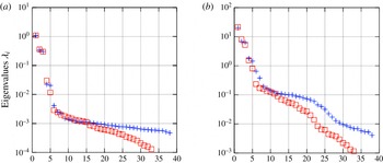
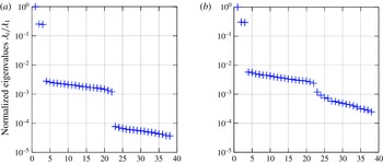
, are used to show the eigenvalues convergence. Figure 10 shows the spectrum
 ${\it\Lambda}$
for both the weakly (Wcase) and the strongly (Scase) coupled cases. The most relevant eigenvalues converge rapidly:
 $M=50$
gradients are sufficient to predict correctly the spectrum
 ${\it\Lambda}$
in the 38-dimension probabilistic space. First, the value of
 ${\it\lambda}_{1}$
, associated with the mean variation of the growth rate in the strongest direction, is a good indicator on how the annular configuration is sensitive to the input uncertainties: figure 10 reveals that the strongly-coupled case is much more sensitive than the weakly-coupled case by two orders of magnitude. Second, for the two cases, only the first five eigenvalues are relevant (e.g. keeping only eigenvalues larger than
 $1\,\%$
of
 ${\it\lambda}_{1}$
), suggesting that the UQ problem can be reduced from a 38-dimensional to a
 $5$
-dimensional problem. Breaking the ‘dimensional curse’ is desirable in this problem, especially for the Scase for which no theoretical simplification is available (i.e. the risk factor has to be assessed numerically).
Eigenvalues
 ${\it\Lambda}$
for the weakly (Wcase, a) and strongly (Scase, b) coupled cases using
 $M_{1}=50$
samples (red square) or
 $M_{1}=500$
samples (blue cross).

The new inputs are the
 $D$
linear combinations
 $\mathscr{H}_{k}=W_{k}^{T}h$
of the initial variables
 $h=(n_{i},{\it\tau}_{i})_{i=1,\ldots ,19}$
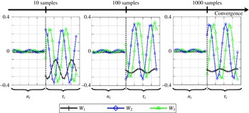
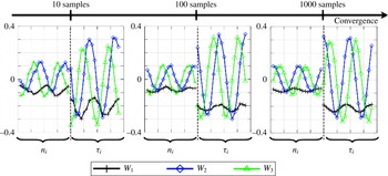
, displayed for both the weakly and strongly-coupled regimes in figures 11 and 12. It is worth noting that coefficients
 $W_{k}^{T}$
associated with the FTF amplitude
 $n_{i=1,\ldots ,N}$
are almost null for Wcase but not for Scase: weakly-coupled modes are essentially controlled by the time delays while both
 $n_{i}$
and
 ${\it\tau}_{i}$
are necessary for strongly-coupled cases. This is a fundamental result since usually only time delays are assumed to control the stability of thermoacoustic modes, a result which is valid only for weakly-coupled modes. The natural next question is the physical interpretation of the active variables: are they only mathematical ingredients or do they convey any physical meaning?
Three first eigenvector
 $W_{k=1,\ldots ,3}$
coefficients of the Wcase case associated to the
 $N=19$
uncertain gains
 $n_{i=1,\ldots ,19}$
time delays
 ${\it\tau}_{i=1,\ldots ,19}$
. The eigenvectors convergence is displayed for
 $M_{1}=10$
, 100 and 1000 samples.

Three first eigenvector
 $W_{k=1,\ldots ,3}$
coefficients of the Scase case associated to the
 $N=19$
uncertain gains
 $n_{i=1,\ldots ,19}$
time delays
 ${\it\tau}_{i=1,\ldots ,19}$
. The eigenvectors convergence is displayed for
 $M_{1}=10$
, 100 and 1000 samples.

The first eigenvector (
 $W_{1}$
in figure 11) converges to an equi-weighted linear combination for Wcase, associated with the mean flame transfer function over the
 $N=19$
burners. A similar trend is observed for Scase even if 1000 samples are not sufficient to ensure a complete convergence. However, the two other eigenvectors (
 $W_{2}$
and
 $W_{3}$
in both figures 11 and 12) have more complex behaviours which have to be analysed. To do so, the theoretical background derived in § 2.2 for annular configurations with no plenum can be used. Equation (2.12) has shown that a weakly-coupled annular cavity is characterized by two parameters: (i) the coupling strength
 ${\it\Sigma}_{0}$
, associated with the mean flame over the
 $N$
burners and (ii) a splitting strength
 $\mathscr{S}_{0}$
, which involves two coefficients of the Fourier transform
 $\widehat{{\it\Gamma}_{4}^{0}}$
:
 $\widehat{{\it\Gamma}_{4}^{0}}(2p)$
and
 $\widehat{{\it\Gamma}_{4}^{0}}(-2p)$
, where
 $p$
is the azimuthal mode order (
 $p=1$
here). In simple situations where the flames are located at the burner/chamber junction (
 ${\it\alpha}=1$
), the coupling parameter
 ${\it\Gamma}_{i,4}^{0}$
, defined in (2.7), reduces to
 $$\begin{eqnarray}{\it\Gamma}_{4,i}^{0}=-\frac{1}{2}\frac{S_{i}}{S_{c}}\frac{{\it\rho}^{0}c^{0}}{{\it\rho}_{u}^{0}c_{u}^{0}}\text{ cotan}\left(\frac{{\it\omega}^{0}L_{i}}{c_{u}^{0}}\right)[1+\mathscr{F}_{i}({\it\omega}^{0})],\end{eqnarray}$$
where
 $\mathscr{F}_{i}=n_{i}\text{e}^{j{\it\omega}^{0}{\it\tau}_{i}}$
is the flame transfer function of the
 $i$
th flame evaluated at the pulsation
 ${\it\omega}^{0}={\rm\pi}c^{0}/L_{c}$
. Thus
 $\widehat{{\it\Gamma}_{4}^{0}}$
is associated with the spatial Fourier transform of the flame pattern
 $\widehat{\mathscr{F}}(k)=\sum _{i=1}^{N}\mathscr{F}_{i}\text{e}^{-j2{\rm\pi}k\text{i}/N}$
, i.e. the azimuthal distribution of the FTFs. Note that
 $\widehat{\mathscr{F}}(k)$
corresponds to a pattern with a period
 $N/k$
.
Consequently, the theory of symmetry breaking (Bauerheim et al.
Reference Bauerheim, Salas, Nicoud and Poinsot2014e
) suggests that, in the weakly-coupled regime, active variables are linked to the 0th and
 $\pm 2p$
th coefficients of the spatial Fourier transform
 $\widehat{\mathscr{F}}$
. It is worth noting that for the first azimuthal mode (
 $p=1$
), the two eigenvectors
 $W_{2}$
and
 $W_{3}$
displayed in figures 11 and 12 exhibit a periodic behaviour of period
 $N/2$
, suggesting a direct link between the eigenvectors
 $W_{2}$
and
 $W_{3}$
and the coefficients
 $\widehat{\mathscr{F}}(\pm 2)$
. Note also that the mean flame, and therefore the eigenvector
 $W_{1}$
, is linked to the
 $0$
th coefficient of the Fourier transform
 $\widehat{\mathscr{F}}(0)$
. These theoretical findings suggest that a change of variables could be used to ease the physical interpretation of active variables in figures 11 and 12, as well as to improve the accuracy of the eigen-decomposition:
 $$\begin{eqnarray}\{n_{i},{\it\tau}_{i}\}\Rightarrow \{\text{Re}(\widehat{\mathscr{F}}),\text{Im}(\widehat{\mathscr{F}})\}.\end{eqnarray}$$
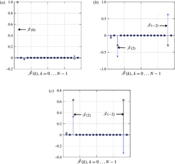
Results for Wcase (a) and Scase (b) are displayed in figure 13. They show a reduction of the active subspace from 5 before (where inputs were
 $n_{i}$
and
 ${\it\tau}_{i}$
) to only 3 for both cases because a physical nonlinear combination of the inputs (
 $n_{i}\text{e}^{j{\it\omega}^{0}{\it\tau}_{i}}$
) were introduced (note that the active subspace approach can only search for linear combinations of the input variables). This result highlights the benefit of using theory to guide UQ strategies. Indeed, the associated active variables, shown in figure 14, demonstrate that the effect dominating the growth-rate response corresponds to the coupling strength and splitting strength, involving the 0th and
 $\pm 2$
th Fourier coefficients of the flame transfer-function distribution. Other coefficients play a minor role especially for the weakly-coupled regime. It is striking to see that the active subspace method actually recovers the parameters exhibited in the weak coupling limit provided by the analytical derivation of ATACAMAC: the coupling and the splitting strength. Nevertheless, while
 $\mathscr{H}_{1}$
can be directly linked to the coupling strength, the formal relationship between the two other active variables
 $\mathscr{H}_{2}$
and
 $\mathscr{H}_{3}$
and the analytical splitting strength cannot be obtained. Consequently, an EM algorithm is used in § A.2 to show that
 $\mathscr{H}_{2}$
and
 $\mathscr{H}_{3}$
are associated with a splitting effect, i.e. to the variable
 $Z=\pm 1$
of the EM algorithm. This UQ technique also shows that the strongly-coupled regime is controlled by these three same active variables, and therefore by a coupling and splitting strength, a result which was not available theoretically. A crucial question is therefore to understand the differences between the weakly and strongly-coupled regimes. If it is not on the underlying parameters, as shown in this section, it might be on the nature of the response surface itself. This issue is addressed in § 4.2.
Normalized eigenvalues
 ${\it\lambda}_{i}/{\it\lambda}_{0}$
for the weakly (a) Wcase and strongly (b) Scase coupled cases using 500 samples.

Real (square) and imaginary (cross) parts of the three first eigenvectors
 $W_{i}$
obtained by the active subspace approach combined with a change of variable defined by (4.2) for the weakly-coupled case with 1000 samples.

4.2. Response surface approximation
The active subspace approach, applied in § 4.1 (figure 9
a), has provided successful results by reducing the 38-dimensional input space into a low-dimension subspace for both the weakly and the strongly-coupled cases. The next question is: how to exploit this dimension reduction? Indeed, a Monte Carlo technique cannot be directly performed on the active subspace since it is difficult to determine the PDFs of
 $\mathscr{H}_{i}$
knowing the PDF of
 $n_{i}$
and
 ${\it\tau}_{i}$
. One straightforward option is to approximate the surface response
 $f_{Im}$
by a surrogate model
 $\widetilde{f_{Im}}$
(figure 9
b). Only the maximum growth rate of the two azimuthal components is considered here (see § A.2 for a surrogate model with the two components put together). This approximation procedure suffers from the ‘curse of dimensionality’, so it may benefit tremendously from proper dimension reduction as proposed in this paper. Here, linear, quadratic and cubic polynomials are chosen on the full and reduced spaces (
 $D_{sm}=3$
or 38, where
 $D_{sm}$
is the number of active variables retained) to construct such surrogate models:
 $$\begin{eqnarray}\widetilde{f_{Im}}=\underbrace{a_{0}+\mathop{\sum }_{j=1}^{D_{sm}}b_{j}\mathscr{H}_{j}}_{\text{Linear (L)}}+\underbrace{\mathop{\sum }_{j=1}^{D_{sm}}\mathop{\sum }_{k=j}^{D_{sm}}c_{j,k}\mathscr{H}_{j}\mathscr{H}_{k}}_{\text{Quadratic (Q)}}+\underbrace{\mathop{\sum }_{j=1}^{D_{sm}}\mathop{\sum }_{k=j}^{D_{sm}}\mathop{\sum }_{l=k}^{D_{sm}}d_{j,k,l}\mathscr{H}_{j}\mathscr{H}_{k}\mathscr{H}_{l}}_{\text{Cubic (C)}},\end{eqnarray}$$
where
 $\mathscr{H}_{i}$
is the
 $i$
th active variable defined as
 $\mathscr{H}_{i}=W_{i}^{T}h$
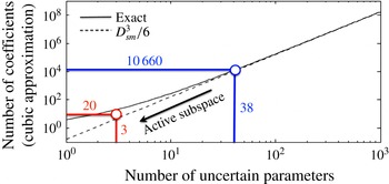
. As shown in figure 15, this surface approximation constitutes a classical but challenging approach, which suffers from the ‘curse of dimensionality’. Indeed, the number of coefficients, obtained by least squares regressions for instance, evolves roughly like
 $D_{sm}^{3}/6$
for a cubic approximation. An exact determination of this complexity is given by
 $$\begin{eqnarray}\displaystyle \left.\begin{array}{@{}c@{}}N_{L}=1+D_{sm},\quad N_{L+Q}=1+2D_{sm}+{\textstyle \frac{1}{2}}D_{sm}(D_{sm}-1),\\ N_{L+Q+C}=1+3D_{sm}+{\textstyle \frac{3}{2}}D_{sm}(D_{sm}-1)+\frac{1}{6}D_{sm}(D_{sm}-1)(D_{sm}-2).\end{array}\right\} & & \displaystyle\end{eqnarray}$$
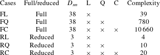
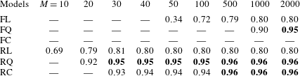
Consequently, prior to computing risk factors, the response surface is approximated using (4.3) in six cases with different complexity, in order to highlight benefits of the dimension reduction. These cases are summarized in table 3. For each case, a least square regression is performed on
 $M$
samples, from
 $M=10$
to
 $M=2000$
. The approximated surrogate model
 $\widetilde{f_{Im}}$
is then replayed randomly 10 000 times on a Monte Carlo dataset corresponding to the weakly-coupled case (Wcase) and then the strongly-coupled case (Scase). Results are compared to the true response surface
 $f_{Im}$
obtained by ATACAMAC. This study constitutes a validation of the complete methodology proposed in this paper, allowed by the ATACAMAC tool which can efficiently compute true response surfaces on large Monte Carlo datasets. The accuracy of the fitted response surface is evaluated by the variance of the error
 $$\begin{eqnarray}R=1-\frac{\text{Var}(\widetilde{f_{Im}}-f_{Im})}{\text{Var}(f_{Im})},\end{eqnarray}$$
where
 $\text{Var}(\widetilde{f_{Im}}-f_{Im})$
is the variance of the error over the 10 000 validation samples, normalized by the variance of the true response surface
 $\text{Var}(f_{Im})$
.
Exact (——) and approximate (- - - -) number of coefficients in the cubic approximation of the response surface
 $\widetilde{f_{Im}}$
(4.3) versus the number of uncertain parameters
 $D_{sm}$
. The complexity of this problem increases drastically with
 $D_{sm}$
, which justifies the need of the active subspace approach.

Several surrogate models to approximate the surface response
 $\widetilde{f_{Im}}$
on the full and reduced spaces.


Results for the weakly-coupled regime (Wcase) are displayed in table 4 and figure 16 (only 500 samples per case are shown), which reveal the significant benefits due to the reduced active subspace. Indeed, the surrogate model requires too many coefficients when approximated in the full initial space (
 $D_{sm}=38$
, in blue):
 $39$
(L),
 $780\;(\text{L}+\text{Q})$
and
 $10\,660\;(\text{L}+\text{Q}+\text{C})$
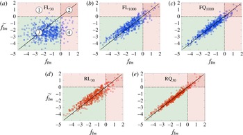
. Consequently, a dataset with less than hundreds of samples cannot even estimate properly the growth-rate linear variations (e.g.
 $\text{FL}_{30}$
in figure 16). As shown in table 4, 95 % accuracy is achieved only when using a quadratic model (780 coefficients) and therefore requires a tremendous effort with numerous simulations: at least 2000, which is not feasible with acoustic or LES solvers. Table 4 also reveals that the cubic approximation does not improve the results. This has been tested for an order up to five, which suggests that a part of the response surface is not polynomial (the last 4 % error). Note that this error cannot be due to the dimension reduction, since the polynomial fitting has been also applied to the full models (FL, FQ and FC cases, which incorporate all the 38 variables), so that the polynomial fitting remains the only source of error in the problem.
Comparison between approximated (
 $\widetilde{f_{Im}}$
) and true (
 $f_{Im}$
) response surfaces in the weakly-coupled regime (Wcase) using different models (
 $\text{L}=\text{linear}$
and
 $\text{Q}=\text{quadratic}$
), different number of samples (
 $M=30$
and 1000) and different input spaces (full in blue, (a–c) and reduced in red, (d,e)). —— Corresponds to the ideal case were the surrogate model is equal to the true response surface (
 $\widetilde{f_{Im}}=f_{Im}$
); - - - - indicates the stability limits
 $f_{Im}=0$
and
 $\widetilde{f_{Im}}=0$
. Ideally, no data should be in zones 1 and 4. Zone 2 corresponds to correct unstable predictions whereas zone 3 is associated with correct stable predictions.

Since only three active variables are supposedly controlling the main growth-rate variations (figure 13), a surrogate model can be constructed on the reduced space (
 $D_{sm}=3$
, in red) with much less effort. Indeed, the number of coefficients to be evaluated is: 4 (L),
 $10\;(\text{L}+\text{Q})$
, and
 $20\;(\text{L}+\text{Q}+\text{C})$
. Thus, linear variations of the response can be obtained with only 30 simulations (
 $\text{RL}_{30}$
in figure 16). Nevertheless, a linear model (L) is not sufficient to approximate this response surface, because of the nonlinearities induced by the flame transfer function and the symmetry-breaking effects. To improve the accuracy of the surrogate models, the order of the polynomials must be increased, which increases the number of coefficients as well. Even if it was prohibitive in high dimensions (
 $D_{sm}=38$
), the reduced active subspace offers more possibilities (figure 15): a quadratic model only requires 10 coefficients and a cubic only 20. As illustrated in figure 16, this yields accurate response surface (96 %) with only 30 simulations, while at least 1000 computations were necessary in the full space to estimate only linear variations.
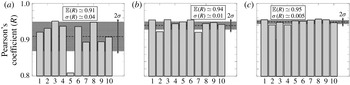
To complement table 4 and figure 16, the variability and predictions of the quadratic low-order models using the active subspace space approach (namely
 $\text{RQ}_{20}$
,
 $\text{RQ}_{30}$
and
 $\text{RQ}_{40}$
) are studied in detail in figure 17. To do so, the active subspace estimation (step in figure 9
a) and the surface response approximation (step in figure 9
b) are performed with several dataset sizes (
 $M=20$
, 30 and 40), as for table 4. However, now for each size
 $M$
, the whole procedure is carried out 10 times. Then, all low-order models generated are validated against the same ATACAMAC dataset containing
 $M_{v}=10\,000$
computations (step in figure 9
c). Results (the correlation coefficients
 $R$
, obtained in (4.5)) are compared for the three different models in figure 17. The mean and standard deviation of the Pearson’s coefficient highlight the accuracy and variability of the low-order models considered. In particular, they show that with only a few simulations (40 computations, to be compared with the large number of uncertain parameters in the initial problem, i.e. 38 dimensions), a high accuracy (
 $\mathbb{E}(R)\simeq 95\,\%$
) and a low variability (
 ${<}0.5\,\%$
) can be achieved. It highlights how the dimension reduction can lead to efficient UQ strategies even in high dimensions.
For each dataset size
 $M$
(20, 30 and 40), the whole approximation procedure (steps in figure 9(a–c)) is performed 10 times. The mean (- - - -) and standard deviation (
 $\cdots \cdots$
) of the Pearson’s coefficient
 $R$
are displayed showing the accuracy (
 $\mathbb{E}(R)$
) and the variability (corresponding to the grey zone at
 $\mathbb{E}(R)\pm {\it\sigma}(R)$
) of the models considered. The reduced method based on the active subspace method is found to converge rapidly with a high accuracy (
 $\mathbb{E}(R)\simeq 95\,\%$
) and a low variability (
 ${<}0.5\,\%$
). This is achieved with only a few simulations regarding the high dimension of the initial problem.

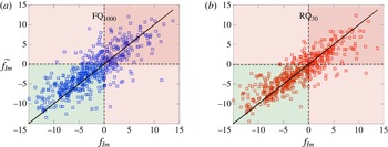
Similar behaviours are obtained in the strongly-coupled regime, but with lower accuracies (63 % in the full initial space with the model
 $\text{FQ}_{1000}$
, and 75 % in the active subspace with
 $\text{RQ}_{30}$
). Figure 18 shows a comparison between these quadratic models in the full (requiring 1000 samples) and reduced spaces (30 simulations). This result unveils interesting information on the underlying physics controlling the strongly-coupled regime, while no theoretical background is available today for this case:
-
(i) The active subspace approach (figure 13) revealed that the strongly-coupled regime, as the weakly one, is controlled by the coupling strength (
${\it\Sigma}_{0}$
) and splitting strength (
$\mathscr{S}_{0}$
). Other parameters have minor effects. -
(ii) The response surface approximations unveil that, compared with Wcase where the error was less than 4 %, polynomial models are not suited for Scase, since 25 % of the variance is still not explained.


These two points suggest that the strongly-coupled regime, which occurs due to a bifurcation in the system, is controlled by a non-polynomial response surface. Other techniques could be efficiently applied on this case using benefits of the active subspace and the three active variables, to discover the nature of the response surface in the strongly-coupled regime.
Comparison between approximated (
 $\widetilde{f_{Im}}$
) and true (
 $f_{Im}$
) response surfaces, similar to figure 16, but in the strongly-coupled regime (Scase). 30 simulations in the reduced subspace (red, b) provide better results than 1000 computations in the full initial space (blue, a).

4.3. Risk-factor assessment
Finally, predictions of the risk factors associated with the first azimuthal mode of the annular combustor are obtained with both surrogate models and direct Monte Carlo analysis (appendix A). Section A.2 describes a Monte Carlo analysis and an algorithm to treat the two components together. Since it yields more complex surrogate models, only the maximum growth rate is considered here for the sake of simplicity.
The risk factor being defined as the integration of a PDF function (3.2), some errors may cancel out leading to more accurate risk-factor estimations than for PDFs. However, in cases where the risk factor is low, only the PDF tail is integrated, corresponding to rare events, which may yield bad predictions of the instability probability. Consequently, this section intends to investigate the risk-factor estimation by low-order models (steps in figure 9
a,b) when replayed
 $M_{v}$
times (step in figure 9
c).
First, the quadratic low-order models
 $\text{RQ}_{30}$
and
 $\text{RQ}_{1000}$
are replayed
 $M_{v}$
times for the weakly-coupled case to estimate the growth rate PDF and the risk factor (step in figure 9
c). The database size for the model estimation is therefore
 $M=30$
and
 $M=1000$
(steps in a and b) to ensure an accurate and robust model (table 4), while the number
 $M_{v}$
of replay (step in c) is varied from 100 to 50 000. The convergence analysis (figure 19) suggests that 20 000 computations of these low-order models are required to provide accurate and robust estimation of the risk factor. Note that this step in (
 $c$
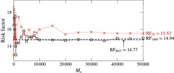
) does not require heavy computational resources since only algebraic models are replayed (about 1 min for 10 000 replay on a standard laptop). Moreover, it shows that such a low-order model provides a good approximation of the risk factor (▫ in figure 19), compared with the Monte Carlo analysis using ATACAMAC (- - - -, appendix A) considered as the true risk-factor estimation. Using only 30 simulations (
 $\times$
in figure 19) leads to a small but reasonable error on the risk-factor estimation (relative error below 5 %).
Convergence of the low-order models
 $\text{RQ}_{30}$
(
 $\times$
) and
 $\text{RQ}_{1000}$
(▫) when it is replayed
 $M_{v}$
times. These models yield a good agreement for the risk factor (RF) compared with the Monte Carlo analysis using ATACAMAC (- - - -, appendix A) for
 $M_{v}>20\,000$
(low variability). A small error (
 ${<}5\,\%$
) occurs however when using only
 $M=30$
simulations for the surface approximation.

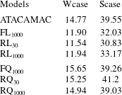
Risk factors computed by several surrogate models (
 $\text{FL}_{1000}$
,
 $\text{RL}_{30}$
,
 $\text{RL}_{1000}$
,
 $\text{FQ}_{1000}$
,
 $\text{RQ}_{30}$
and
 $\text{RQ}_{1000}$
). They are compared with a reference value obtained by a direct Monte Carlo analysis on the full space by ATACAMAC (appendix A).

Using a similar analysis, other surrogate algebraic models (table 3, figure 9
b) are replayed 20 000 times to estimate the risk factor of the first circumferential mode of the combustor (figure 9
c), in both the weakly (Wcase) and strongly (Scase) coupled cases. They are compared with the reference risk factor evaluated by ATACAMAC (10 000 simulations). Results given in table 5 demonstrate that the novel UQ technique proposed here can estimate efficiently and accurately the probability of the mode to be unstable. As expected, quadratic models lead to better estimations than linear models. In particular, the low-dimensional active subspace leads to precise stability predictions with only 30 simulations (model
 $\text{RQ}_{30}$
), with relative errors of 3.2 % (Wcase) and 4.0 % (Scase). Further analysis of the splitting effects on the risk factor is studied by an EM algorithm in appendix A (figure 21).
5. Conclusion
For the first time, uncertainty quantification has been applied on the thermoacoustic stability of two annular cavities coupled by 19 flames, to determine its modal risk factor defined as the probability of a mode being unstable. In particular, this paper focuses on the symmetry-breaking effects induced by uncertainties, already known to destabilize the configuration in a deterministic framework. However, when considering 2 uncertain parameters per flame (e.g. the gain and time delay of the flame transfer function), it yields a large nonlinear UQ problem with 38 random variables prone to bifurcations. To tackle this well-known ‘curse of dimensionality’, a novel UQ methodology is applied. It relies on the active subspace approach to construct a reduced set of input variables. This strategy is applied on two annular coupled cavities using an acoustic-network model, which is solved quasi-analytically. Results show that the dimension of the probabilistic problem can be drastically reduced, from 38 uncertain parameters to only 3. This is desirable since working with 38 dimensions is usually too expensive, even for acoustic solvers. Moreover, it is found that the three active variables are related to physical quantities, which unveils underlying phenomena controlling the stability: the first active variable is associated with a coupling strength controlling the bifurcation of the system, while the two others correspond to a symmetry-breaking effect on the azimuthal modes. This symmetry reduction and associated destabilization effect appears due to the non-uniform pattern of the uncertainty distribution. Finally, the dimension reduction is exploited by constructing surface responses with polynomials (linear, quadratic and cubic). This approximation procedure, for which the complexity evolves like
 $D_{sm}^{3}/6$
for a cubic model with
 $D_{sm}$
variables, suffers from the ‘curse of dimensionality’, and therefore may benefit tremendously from the proper dimension reduction obtained here. By comparing accuracy and cost, the results prove that 5 % error on the risk factor can be achieved with only 30 simulations on the reduced space, whereas 2000 are required on the complete initial space. This surrogate algebraic models are then replayed 50 000 times at low cost to estimate the risk factor of the system. They are compared with a reference risk factor obtained directly by ATACAMAC using 10 000 Monte Carlo simulations. It yields very good approximations of the risk for both the weakly and strongly-coupled regimes, adding that only 30 ATACAMAC simulations have been used to construct the quadratic algebraic model. This exemplifies that this novel UQ method can accurately predict the risk factor of an annular configuration at low cost, and constitutes an innovative approach in thermoacoustics.
Acknowledgements
Authors gratefully acknowledge Professor Iaccarino for his help and fruitful discussions during the CTR Summer Program 2014. Part of this study was performed within the UMRIDA research program (contract no. FP7-AAT-2013-RTD-1-605036) funded by the European Community.
Appendix A. Monte Carlo analysis using ATACAMAC
A.1. Maximum growth-rate estimation by Monte Carlo
A Monte Carlo analysis is performed using 10 000 ATACAMAC simulations for both the weakly and strongly-coupled modes. Only the maximum growth rates of the two components of the azimuthal mode are considered here (see § A.2 for a study of the two azimuthal components together). The Monte Carlo technique allows a robust estimation of the growth-rate PDFs and risk factors, but requires a prohibitive computational cost. Such a study cannot be achieved with more expensive tools such as 3-D Helmholtz solvers or LES. In this paper, this Monte Carlo analysis is used as a reference database to evaluate the accuracy of the reduced UQ strategy based on the active subspace approach. Figure 20 shows the result of this Monte Carlo analysis. The risk factor is computed for each case and is considered as a reference value in this paper:
 $\text{RF}(\text{Wcase})=14.77\,\%$
and
 $\text{RF}(\text{Scase})=39.55\,\%$
.
Monte Carlo analysis using 10 000 ATACAMAC simulations for both the weakly (a,b) and strongly (c,d) coupled cases. Each point on the stability map (a,c) corresponds to one ATACAMAC simulation. This method allows a robust estimation of PDFs and risk factors (b,d), but requires a prohibitive cost.

A.2. Segregation of the azimuthal mode components in the Monte Carlo analysis
To unravel the two different components of the azimuthal mode in the Monte Carlo analysis (figure 20), an EM (estimation–minimization Dempster & Laird (Reference Dempster and Laird1977)) algorithm for incomplete data is applied on the ATACAMAC results. It is based on a two-step algorithm:
-
(1) Initialization. A variable
$Z$
is initialized randomly with value
$\pm 1$
. -
(2) Step E. Similarly to (4.3), a linear surrogate model is fit on the data, based on the three active variables (
$D_{sm}=3$
), but also on the variable
$Z$
. The variable
$Z$
is affected only by active variables corresponding potentially to splitting terms, i.e.
$\mathscr{H}_{2}$
and
$\mathscr{H}_{3}$
, but not
$\mathscr{H}_{1}$
which is associated with the coupling strength. (A 1)This model corresponds to a model where
$$\begin{eqnarray}\widetilde{f_{Im}}=a_{0}+b_{1}\mathscr{H}_{1}+Z\mathop{\sum }_{j=2}^{D_{sm}}b_{j}\mathscr{H}_{j}.\end{eqnarray}$$
$\sum _{j=2}^{D_{sm}}b_{j}\mathscr{H}_{j}$
is a splitting strength, since
$Z$
can only take values
$+1$
or
$-1$
. The term
$b_{1}\mathscr{H}_{1}$
, independent of the
$Z$
variable, is the coupling strength and does not depend on the FTF pattern but only on the mean FTF.
-
(3) Step M. The previous step has produced an estimation of the model coefficients
$a_{0}$
and
$b_{j}$
. This model and the data can then be reused to evaluate a new variable
$Z$
thanks to a minimization procedure: for each data, the variable
$Z$
is changed into
$-Z$
. If this new value yields a better estimation, this value is retained. -
(4) Iteration. At the end of Step M, a new vector
$\boldsymbol{Z}$
is produced. Consequently, a new step
$E$
can be performed, leading to an iterative method to obtain both the model (coefficients
$a_{0}$
and
$b_{j}$
) and the segregation between the two components of the azimuthal mode (given by
$\boldsymbol{Z}$
). The convergence of such an iterative algorithm is not ensured and therefore should be monitored.


The two different components (
 $\times$
when
 $Z=+1$
and ○ when
 $Z=-1$
) of the azimuthal modes obtained by the variable
 $\boldsymbol{Z}$
in the EM algorithm (a). For this weakly-coupled case, the convergence is monitored by the Pearson’s coefficient
 $R$
at each iteration step in (b). The splitting is observed by the shift between the mean location of the two clouds of points (white circle and cross).
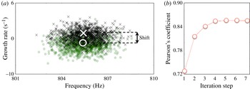
Results of the EM algorithm for the weakly-coupled case are shown in figure 21. The two split components (
 $\times$
and ○) are determined (a). It shows that a strong splitting effect occurs and destabilizes the configuration. Even though this splitting has a probabilistic nature, its statistical mean value is not null (mean shift displayed in figure 21). This exemplifies the nonlinear behaviour of symmetry breaking, where the system is symmetric ‘in average’ (FTFs are modified around the symmetric case), but symmetry breaking induces a non-zero averaged splitting strength, yet not present in the ‘averaged symmetric’ configuration. This result illustrates the need to perform UQ analysis to capture such effects affecting the mean stability of the configuration which are not present in deterministic studies. The convergence of the EM algorithm is also displayed (b) by monitoring the Pearson’s coefficient at each iteration step. The final model accuracy is similar to other models investigated in the paper (
 $R\simeq 85.4\,\%$
). From this analysis, it can be inferred that the two active variables
 $\mathscr{H}_{2}$
and
 $\mathscr{H}_{3}$
are associated with a random splitting effect, as expected using the analytical results of Bauerheim et al. (Reference Bauerheim, Salas, Nicoud and Poinsot2014e
) in the weakly-coupled regime.
Nomenclature
-
$f$
-
Complex frequency
-
${\it\omega}$
-
Complex pulsation
-
$f_{Im}=\text{Im}(f)$
-
Growth rate
-
$\widetilde{f_{Im}}$
-
Growth-rate estimation
-
$N$
-
Number of burners
-
$\text{LES}$
-
Large eddy simulation
-
$\text{ATACAMAC}$
-
Low-order acoustic tool for azimuthal modes
-
$\text{AVSP}$
-
3D Helmholtz solver
-
$p^{\prime }$
-
Acoustic pressure
-
$\hat{p}$
-
Acoustic pressure FFT
-
$u^{\prime }$
-
Acoustic azimuthal velocity
-
$\hat{u}$
-
Acoustic azimuthal velocity FFT
-
$w^{\prime }$
-
Acoustic longitudinal velocity
-
${\hat{w}}$
-
Acoustic longitudinal velocity FFT
-
$\dot{{\it\omega}_{T}}^{\prime }$
-
Heat release oscillation
-
$\widehat{\dot{{\it\omega}_{T}}}$
-
Heat release oscillation FFT
-
$\text{FFT}$
-
Fast Fourier transform
-
$\text{UQ}$
-
Uncertainty quantification
-
$\text{FTF}$
-
Flame transfer function
-
$\text{PDF}$
-
Probability density function
-
$L_{c}$
and
$L_{p}$
-
Half-perimeter of the chamber/plenum cavity
-
$S_{c}$
and
$S_{p}$
-
Cross-section of the chamber/plenum cavity
-
$L_{i}$
-
Length of the
$i$
th burner -
$S_{i}$
-
Section of the
$i$
th burner -
$n_{i}$
-
Gain of the
$i$
th FTF -
${\it\tau}_{i}$
-
Time-delay of the
$i$
th FTF -
${\it\Gamma}_{k=1,\ldots ,4,i}$
-
$k$
th coupling parameter of the
$i$
th sector
-
$\hat{{\it\Gamma}}$
-
Spatial Fourier transform of the coupling parameter distribution
-
${\it\Sigma}_{0}$
-
Coupling strength
-
$\mathscr{S}_{0}$
-
Splitting strength
-
$\bar{n}$
and
${\it\sigma}_{n}$
-
Mean and standard deviation of the FTF gain
-
$\bar{{\it\tau}}$
and
${\it\sigma}_{{\it\tau}}$
-
Mean and standard deviation of the FTF time-delay
-
$h_{i}$
-
Initial uncertain parameters (
$n_{i}$
’s or
${\it\tau}_{i}$
’s) -
$\mathscr{H}_{i}$
-
Active variables
-
${\it\Lambda}$
-
Spectrum produced by active subspace
-
$W_{i}$
-
$i$
th eigenvector produced by active subspace
-
$\boldsymbol{{\rm\nabla}}_{h}^{k}f_{Im}$
-
$k$
th sample of the growth-rate gradient in the
$i$
th direction
-
$M$
-
Number of estimation points
-
$M_{v}$
-
Number of validation points
-
$\unicode[STIX]{x1D63E}$
-
Uncentred covariance matrix of the gradients
-
$D$
-
Dimension of the UQ problem
-
$D_{sm}$
-
Dimension of the surrogate model
-
$R$
-
Pearson’s coefficient
-
$\text{RF}$
-
Risk factor