2.1. Configuration and parameters

The geometry of the bullet-shaped blunt body moving in a tube and the main geometrical parameters are shown in figure 1. The body consists of a half-ellipsoid nose glued to a cylindrical rear. The diameter of the cylinder is referred to as $d$. The ellipsoid of revolution is defined by its major axis with $a_x = 2a_y = d$ and its minor axis which fits with the cylindrical section by imposing $a_y = a_z = d/2$.

The diameter of the pipe is noted as $D$, so that the effect of confinement will be defined by either a diameter ratio $\xi = d/D$ or an area ratio $a/A = \xi ^2$, with $a={\rm \pi} d^2/4$ the frontal area of the body and $A ={\rm \pi} D^2/4$ the area of the tube.

The origin of the frame is taken at the junction between half-spheroidal and cylindrical parts, so that the body spans from $x=-d$ (nose) to $x=L-d$ (base).

The object moves with a velocity $U$ in the direction $-\boldsymbol {e}_x$ and the wall of the pipe is fixed. Assuming the flow is incompressible and isothermal, the non-dimensional parameters of this problem are the Reynolds number $Re= \rho U d / \mu$, the diameter aspect ratio $\xi =d/D$ and the length aspect ratio $L/d$. Here $\rho$ and $\mu$ are respectively the constant density and dynamic viscosity of the fluid. In most cases the parameter $L/d$ will be set to $2$, except in § 3.3 where the effect of this parameter will be investigated.

The study will be conducted in the frame of reference associated to the body. The boundaries of the computational domain are given in figure 1. It is limited by, respectively, an inlet section $S_{inlet}$ and an outlet section $S_{outlet}$. In this frame, the body is fixed, and placed within an incoming flow $U$ of direction $+ \boldsymbol {e}_x$ and the tube wall also moves at the same velocity with respect to the body. Hence, the dimensionless incompressible Navier–Stokes equations and associated boundary conditions are

(2.1a)\begin{gather} \partial_t\boldsymbol{u} =\mathcal{NS}([\boldsymbol{u},p])\equiv{-} \boldsymbol{u}\boldsymbol{\cdot}\boldsymbol{\nabla}\boldsymbol{u} -\boldsymbol{\nabla} p + \frac{2}{Re}\boldsymbol{\nabla} \boldsymbol{\cdot} \boldsymbol{\mathsf{D}}(\boldsymbol{u}), \end{gather}

(2.1b)\begin{gather}\boldsymbol{\nabla}\boldsymbol{\cdot}\boldsymbol{u}=0 , \end{gather}

(2.1c)\begin{gather}\boldsymbol{u}|_{S_{body}}=\boldsymbol{0}, \end{gather}

(2.1d)\begin{gather}\boldsymbol{u}|_{S_{inlet}\cup S_{wall} }=\boldsymbol{e}_x, \end{gather}

(2.1e)\begin{gather}{\left[{-}p{\boldsymbol e}_x +\frac{2}{Re}\boldsymbol{\mathsf{D}}(\boldsymbol{u}) \boldsymbol{\cdot} {\boldsymbol e}_x \right]}_{S_{outlet}} =\boldsymbol{0}, \end{gather}

where $\boldsymbol {u}$ is the relative velocity, and $\boldsymbol{\mathsf{D}}({\boldsymbol u})=(\boldsymbol {\nabla } {\boldsymbol u} + \nabla ^T {\boldsymbol u}) / 2$ is the rate-of-strain tensor. The divergence formulation for the viscous terms is related to the choice of the finite element method (FEM) to solve the equations.

The governing equations are non-dimensionalized by the body velocity $U$, the fluid density $\rho$ and the body diameter $d$. The last boundary condition is written as a no-stress condition on the outlet section, which is a convenient choice for an outlet condition with the FEM approach.

2.2. Global LSA

2.2.1. Equations

The global linear stability approach is performed in the line of the now classical approach described, for instance, in Sipp & Lebedev (Reference Sipp and Lebedev2007), Fabre et al. (Reference Fabre, Citro, Ferreira Sabino, Bonnefis, Sierra, Giannetti and Pigou2018). Within the LSA framework, the velocity and pressure are decomposed into a base flow and a small perturbation as

(2.2a,b)\begin{equation} \boldsymbol{u}(r,\varphi,x,t)=\boldsymbol{u}_{b}(r,x)+\epsilon \hat{\boldsymbol{u}}(r,x)\, {\rm e}^{{\rm i} m\varphi+\lambda t},\quad p(r,\varphi,x,t)=p_{b}(r,x)+\epsilon \hat{p}(r,x)\, {\rm e}^{{\rm i} m\varphi+\lambda t}.\end{equation}

Here $[{\boldsymbol u}_b; p_p]$ is the so-called ‘base flow’, namely the solution of the axisymmmetric, time-independent version of (2.1),

(2.3a,b)\begin{equation} \mathcal{NS}([\boldsymbol{u}_b, p_b]) = {\boldsymbol 0} ; \quad \boldsymbol{\nabla} \boldsymbol{\cdot} \boldsymbol{u}_b = 0.\end{equation}

In (2.2a,b) a small-amplitude perturbation of the base flow is assumed in the form of an eigenmode $[ \hat {\boldsymbol {u}}, \hat {p}]$ associated to an eigenvalue $\lambda =\lambda _r + i\lambda _i$. The real part of the eigenvalue is the growth rate. A positive value indicates here an amplification. The imaginary part is a non-dimensional frequency (time oscillation), which is most conveniently represented by the Strouhal number $St = \lambda _i/ (2 {\rm \pi})$ thanks to the non-dimensionalization choices. Fourier decomposition in the azimuthal direction is possible with the axisymmmetric invariance and an azimuthal wavenumber $m\in \mathbb {Z}$ can be added in the exponential wave-like part of the perturbation. Introducing the decomposition (2.2a,b) into the Navier–Stokes equations and linearizing leads to an eigenvalue problem written as

(2.4a)\begin{gather} \lambda \hat{\boldsymbol{u}}=\mathcal{LNS}_{\boldsymbol{u}_b} ([\hat{\boldsymbol{u}}, \hat{p}]), \end{gather}

(2.4b)\begin{gather}\nabla_m\boldsymbol{\cdot}\hat{\boldsymbol{u}}=0, \end{gather}

(2.4c)\begin{gather}\hat{\boldsymbol{u}}|_{S_{inlet}\cup S_{wall}\cup S_{body}} =\boldsymbol{0}, \end{gather}

where $\mathcal {LNS}^m$ is the linearized Navier–Stokes operator defined as

(2.5)\begin{equation} \mathcal{LNS}^m_{\boldsymbol{u}_b}([\hat{\boldsymbol{u}}, \hat{p}]) ={-} \boldsymbol{u}_{b}\boldsymbol{\cdot}\nabla_m\hat{\boldsymbol{u}} - \hat{\boldsymbol{u}}\boldsymbol{\cdot}\nabla_m\boldsymbol{u}_{b} -\nabla_m \hat{p} + \frac{2}{Re}\nabla_m\boldsymbol{\cdot} \boldsymbol{\mathsf{D}}_m(\hat{\boldsymbol{u}}). \end{equation}

Here quantities $\nabla _m$ and $\boldsymbol{\mathsf{D}}_m$ are the gradient and rate-of-strain operators with $\partial _\varphi (\,{\cdot}\,)$ replaced by $i \times m(\,{\cdot}\,)$.

2.2.2. Resolution methods

The resolution methods employed here are essentially similar to those used in recent papers such as Tchoufag et al. (Reference Tchoufag, Fabre and Magnaudet2014), Fabre et al. (Reference Fabre, Longobardi, Bonnefis and Luchini2019), in which stability analysis of axisymmetric incompressible flows were considered.

Thanks to axisymmetry, the base flow velocity is searched in the cylindrical frame $[{\boldsymbol e}_x,{\boldsymbol e}_r,{\boldsymbol e}_\varphi ]$ as ${\boldsymbol u}_b = [u_{b,x}(x,r), u_{b,r}(x,r),~0]$ so that only two components of velocity are kept. On the other hand, for eigenmodes, three components of velocity are needed, i.e. ${\hat u} = [\hat u_{x}(x,r),~ \hat u_{r}(x,r), ~\hat u_{\phi }(x,r)]$. Within this assumption it is enough to consider a two-dimensional numerical domain ($\varOmega$) corresponding to a meridian plane $(x,r)$.

For both base flow equations and linear stability equations, a FEM is used. For this sake, the equations are first turned into a weak form by introducing test functions $\boldsymbol {v}$ and $q$ and a scalar product $\langle \varphi _1,\varphi _2\rangle =\int _\varOmega \overline {\varphi _1}\boldsymbol {\cdot }\varphi _2\,\mathrm {d}\varOmega$. For instance, the weak form of the base flow (2.5) is written as

(2.6)\begin{equation} \forall ({\boldsymbol v},q), \quad \langle\boldsymbol{v}, \mathcal{NS}([\widehat{\boldsymbol{u}_b}, \hat{p}])\rangle +\langle q,\nabla_0\boldsymbol{\cdot} \widehat{\boldsymbol{u}_b}\rangle = 0.\end{equation}

An integration by parts of the viscous terms is afterward performed and their derivation order is reduced. Dirichlet boundary conditions are incorporated by penalization while the stress-free outlet condition is directly satisfied thanks to integration by parts. The nonlinear problem is then solved using an iterative Newton method. The developed form of the base flow equations in cylindrical coordinates and details about the Newton method can be found, for instance, in Tchoufag et al. (Reference Tchoufag, Fabre and Magnaudet2014), Fabre et al. (Reference Fabre, Longobardi, Bonnefis and Luchini2019).

Similarly, the weak form of stability problem yields

(2.7)\begin{equation} \forall ({\boldsymbol v},q), \quad \lambda \langle\boldsymbol{v}, \hat{\boldsymbol{u}}\rangle= \langle\boldsymbol{v}, \mathcal{LNS}_{\boldsymbol{u}_b}^m ([\hat{\boldsymbol{u}}, \hat{p}])\rangle +\langle q, \nabla_m\boldsymbol{\cdot}\hat{\boldsymbol{u}}\rangle,\end{equation}

which after discretization leads to a generalized eigenvalue problem,

(2.8)\begin{equation} \lambda {B}\hat{X}={A}\hat{X}. \end{equation}

A shift-and-invert method is applied to obtain a collection of eigenvalues (typically 10) located closest to a ‘shift’ value taken as a guess of the searched eigenvalues. As usual in such approaches, several values of the ‘shift’ were systematically tested to explore the complex plane and to ensure that no unstable eigenvalue was missed in the study.

The weak form of the stability equations, details about the integration by parts and the construction of matrices $A$ and $B$ can again be found in Tchoufag et al. (Reference Tchoufag, Fabre and Magnaudet2014), Fabre et al. (Reference Fabre, Longobardi, Bonnefis and Luchini2019).

2.2.3. Numerical implementation

All numerical operations (generation and juniper of a mesh, building of matrix operators, Newton iteration for the base flow problem and the shift-invert method for eigenvalue problem) are handled thanks to the finite element software FreeFem++ (Hecht Reference Hecht2012). The FEM discretization is built with the classical Taylor–Hood elements for all computations.

First, a triangular mesh is built using the well-known Delaunay–Voronoi algorithm, and a preliminary base flow and some modes are computed. An adaptive mesh strategy is adopted in order to ensure convergence of results with respect to mesh refinement, as it is described in Fabre et al. (Reference Fabre, Citro, Ferreira Sabino, Bonnefis, Sierra, Giannetti and Pigou2018). Namely, after first computing a base flow and an adjoint eigenmode, the mesh is adapted to both these fields, and the process is repeated twice. To demonstrate the efficiency of this method, we report in table 1 the eigenvalues computed with the adapted mesh and with an even more refined mesh obtained by adapting to both direct and adjoint modes and subsequently splitting all triangular cells in four. The results demonstrate that the mesh adaptation method provides converged results with a very reasonable mesh density and computational cost.

Table 1.

Comparison of results found with a mesh build with the adaptation strategy and a refined one obtained by splitting. The table reports the number of the leading eigenvalue $\lambda$, the number of mesh vertices $N_v$ and the computational time $t_c$ (on a Macbook, 2Ghz, 32Go RAM, single processor) required for computing 10 modes with the shift-invert strategy, for the set of parameters $Re = 320$, $a/A = 0.75$, $L/d = 2$.

The whole computational chain, including mesh generation, adaptation, loop over parameters and post-processing, is monitored in the Matlab environment thanks to the StabFem suite (Fabre et al. Reference Fabre, Citro, Ferreira Sabino, Bonnefis, Sierra, Giannetti and Pigou2018), which is a set of Matlab/Octave drivers/wrappers specifically designed to perform such studies. A sample script reproducing a selection of results from the present study is available through the website of the stabfem project (https://stabfem.gitlab.io/StabFem).

2.3. Direct numerical simulations

To validate and to extend the results of the stability analysis, some full DNS are performed with the open source computational fluid dynamics software package, OpenFOAM$^{\circledR}$. Time-varying solutions of the (2.1) are computed with its incompressible finite volume solver, pimpleFOAM, built with a second-order spatial derivative scheme and an Euler temporal scheme. A fixed Courant number set to $Co=0.5$ ensures the stability of these schemes. The meshes are built with the cfMesh software provided with OpenFOAM. A typical mesh and a mesh convergence study are presented in Appendix B. Results and comparison with LSA are discussed in § 4.

3.1. $m=\pm 1$ modes for sample values of the section aspect ratio $a/A$

In this section and the next one we set the length-to-diameter aspect ratio $L/d=2$ and we focus on the effect of the confinement ratio $a/A$.

3.1.1. Weakly confined flow

A weakly confined case is first considered, corresponding to section aspect ratio $a/A = 0.01$ (or diameter aspect ratio $d/D = 0.1$). Figure 2 displays the base flow around the blunt body for a Reynolds number $Re=320$. The axisymmetric base flow field exhibits a standing eddy which has approximately the same length as the body itself. The boundary layer present on the body surface is made visible through the generation of negative azimuthal vorticity. Overall, this structure seems to be very similar to that found in Jiménez-González et al. (Reference Jiménez-González, Sevilla, Sanmiguel-Rojas and Martínez-Bazán2014) for the same object and conditions in an unconfined flow.

Figure 2.

Azimuthal vorticity ($\omega _\varphi =\boldsymbol {\nabla } \times \boldsymbol {u}_b \boldsymbol {\cdot } \boldsymbol {e}_\varphi \equiv \partial _x u_r - \partial _r u_x$) and streamlines of the base flow for $Re=320$, $L/d=2$, $a/A=0.01$.

For the same base flow, a part of the spectrum found using the LSA approach is shown in figure 3. It reveals two physical modes, the first one called $S1$ is non-oscillating (often referred to as stationary) and unstable ($\lambda _r>0$). The second one called $01$ is oscillating and damped. The other modes quasi-aligned are some spurious modes of a non-physical nature and come only from the numerical discretization. Similar results are observed by Jiménez-González et al. (Reference Jiménez-González, Sevilla, Sanmiguel-Rojas and Martínez-Bazán2014) for a non-spinning object in unconfined space.

Figure 3.

Example of a spectrum found with the shift and invert algorithm ($Re=320$, $L/d=2$, $a/A=0.01$). The 10 eigenvalues closest to the ‘shift’ value indicated in red are computed.

In their study, the onset of the first instability (the $S1$ mode) was detected at a critical Reynolds number $Re_{c,S1}=325.2$, whereas its value is $Re_{c,S1}=312.2$ in the present study, leading to less than a four percent difference. It can be concluded that the confinement produces a small influence over the onset of the first instability in this case.

Figure 4 displays the four most amplified eigenvalues as a function of $Re$, again for $a/A=0.01$. The first unstable mode appearing is non-oscillating and remains the most amplified mode over the whole range of $Re$ studied. The second most amplified mode, $O1$, becomes unstable at $Re_{c,O1}=478.3$ and $St_c=0.103$. This Strouhal value is very close to the one found by Bohorquez et al. (Reference Bohorquez, Sanmiguel-Rojas, Sevilla, Jiménez-González and Martínez-Bazán2011) who reported $St=0.102$. But the latter authors found a somehow larger value of the critical Reynolds number, namely $Re_{c,O1} = 518$.

Figure 4.

Amplification rate (a) and Strouhal number (b) as a function of the Reynolds number for the first unstable modes, $a/A=0.01$, $L/d=2$.

In addition to the effect of confinement, this gap between critical Reynolds number may be explained by the fact that the computational domain defined for the stability analysis included only the cylindrical rear of the body and excluded the nose in Bohorquez et al. (Reference Bohorquez, Sanmiguel-Rojas, Sevilla, Jiménez-González and Martínez-Bazán2011). The critical Reynolds is also notably higher than the one given by the reference case of a thin disk. The geometry of the nose of the blunt body changes the amount of vorticity produced at its surface, as pointed out by Brücker (Reference Brücker2001), and it is known that this vorticity production is responsible for triggering the instabilities (Magnaudet & Mougin Reference Magnaudet and Mougin2007). Having a profiled nose diminishes such production of vorticity and pushes back the onset of instabilities to larger Reynolds. For instance, in figure 2 the vorticity intensity for $Re = 320$ is $|\omega _\varphi | \approx 10$, which is comparable to the intensity observed for a thin disk with aspect ratio $\chi = 3$ for $Re \approx 150$ as studied in Auguste et al. (Reference Auguste, Fabre and Magnaudet2010).

Up to here, the main scenario revealed in the present configuration by the LSA is a first non-oscillating mode $S1$ amplification followed by an oscillating one $O1$. It is the same encountered for all axisymmetric bodies considered in the literature (Natarajan & Acrivos Reference Natarajan and Acrivos1993; Meliga, Chomaz & Sipp Reference Meliga, Chomaz and Sipp2009b; Tchoufag et al. Reference Tchoufag, Fabre and Magnaudet2014). When pushing the Reynolds number towards higher values, two additional modes are found, an oscillating one and a non-oscillating one termed $O2$ and $S2$. These higher modes arise at much larger Reynolds numbers, in the range $Re \in [900\unicode{x2013}1200]$. They are less likely to be observed experimentally or numerically because in such regimes the mean flow is already very far from the axisymmetric base flow analysed with the linear stability theory. Nevertheless, when the confinement effect is increased, these higher modes turn out to be relevant in order to obtain a consistent picture of the bifurcation scenario. Hence, they will be kept in the analysis and their critical Reynolds $Re_{c,S2}$ and $Re_{c,O2}$ will be tracked.

The structures of these modes are illustrated in figure 5. The plots display both the azimuthal velocity (colours) and pressure (lines) levels in a meridional $(x,r)$-plane (left plots) and the axial vorticity levels in a transverse $(y,z)$-plane corresponding to a cut at location $x=2$ (right plots). The first unstable mode, $S1$, has a rather simple vorticity structure. In the meridional plane, the azimuthal vorticity of the eigenmode is positive in the region of the shear layer. Recalling that the vorticity of the base flow shear layer is negative (see figure 2), the effect of the eigenmode is to decrease in this region the net vortical intensity in the shear layer. Owing to the antisymmetry of $m=\pm 1$ modes, the azimuthal vorticity of the eigenmode is negative on the opposite side, meaning that the shear layer is enhanced. The axial vorticity, on the other hand, reveals a pair of counter-rotating streamwise vortices, as already noticed for disk and spheres (Natarajan & Acrivos Reference Natarajan and Acrivos1993; Meliga et al. Reference Meliga, Chomaz and Sipp2009b) and similar blunt bodies in open flow (Jiménez-González et al. Reference Jiménez-González, Sevilla, Sanmiguel-Rojas and Martínez-Bazán2014). The $S2$ mode shows a similar structure with a small additional pair of counter-rotating vortices in the vicinity of the blunt body rear, and a more complex pressure field than the $S1$ mode.

Figure 5.

Eigenmodes found for $a/A=0.01$, real parts of the vorticity with iso-levels of pressure. Slices are defined by $x=2$ and $r\le 2$. Results are shown for (a) $S1$, $Re=320$; (b) $S2$, $Re=1130$; (c) $O1$, $Re=500$ and (d) $O2$, $Re=950$.

Let us now consider the oscillating modes $O1$ and $O2$ displayed in the bottom part of figure 5. One can observe in an azimuthal plane an alternation of positive and negative streamwise vorticity, which is the signature of unsteady vortex shedding. A shorter spatial wake length scale can be seen for the $O2$ mode, related to its higher shedding frequency (i.e. larger $St$). Note that when observed in a transverse plane, these modes display a characteristic spiral structure. This does not imply that if these modes are present in a nonlinear solution a spiral structure will necessarily be observed. Indeed, it is known that due to the degeneracy associated to mirror symmetry, $m=+1$ and $m=-1$ eigenmodes are mirror images of each other and can lead to two kinds of nonlinear states (Fabre et al. Reference Fabre, Auguste and Magnaudet2008): (i) ‘rotating waves’ corresponding to a pure $m=+1$ (or $m=-1$) eigenmodes with a spiral structure, and (ii) ‘standing waves’ corresponding to superposition of $m=1$ and $m=-1$ eigenmodes characterized by a symmetry plane.

3.1.2. Confined flow with $a/A=0.75$

Let us now consider a more confined flow with a section ratio of $a/A = 0.75$ or a diameter ratio of $d/D = 0.87$. The structure of the base flow and the influence of the tube wall are displayed in figure 6. Compared with the unconfined or weakly confined flow, the recirculation length is shorter as the confinement becomes stronger. For Reynolds number $Re=320$, the flow changes direction close to the pipe wall and goes downstream but without setting a closed recirculation zone attached to the wall, even for large values $Re>320$. The presence of separation in this area is accompanied with a production of negative vorticity. This structure reveals the presence of a confined wall jet. Within the small gap between the body and pipe walls the flow can be seen as parallel and one may expect the flow to be well approximated by a parallel-flow solution called ‘annular Couette–Poiseuille flow.’ This classical solution is reproduced in Appendix A. The theoretical analytical non-dimensional velocity profile is compared in figure 7 to the actual axial flow profile extracted from the base flows represented in figure 6. At location $x= 0.75$ (in the rear part of the afterbody), the observed velocity profile is indistinguishable from the theoretical solution, both for Reynolds numbers $Re=110$ and $320$.

Figure 6.

Azimuthal vorticity and streamlines of the base flow in the moving frame attached to the body for $L/d=2$ and $a/A=0.75$. Top, $Re=110$, bottom $Re=320$.

Figure 7.

Axial velocity $u_x$ as a function to $r$ for $Re=110$ (red) and $Re = 320$ (blue) at locations $x=0.75$ (symbols) and $x=1.25$ (dashed lines). Black dotted line: comparison with annular Poiseuille solution.

The velocity profile at location $x=1.25$, slightly behind the body is also plotted in the figure. The curves show that the velocity profile turns into an annular jet, affected by some diffusion, especially for $Re =110$.

The curves giving the amplification rate and the Strouhal number vs the Reynolds number as computed by the linear stability theory are displayed in figure 8, for the base flow solved with the section aspect ratio $a/A=0.75$.

Figure 8.

Amplification rate $\lambda _r$ (a) and Strouhal number (b) vs the Reynolds number for the first unstable modes, $a/A=0.75$. The horizontal range of the figure corresponds to $Re \in [80\unicode{x2013}1000]$.

Three branches are found as the Reynolds number varies corresponding to two non-oscillating (called again $S1$ and $S2$) and one oscillating mode. The latter is of a distinct nature compared with the modes $O1$ and $O2$ previously encountered. It is characterized by a Strouhal number in a lower range, and it is thus called $O3$. The amplification curves of the $S1$ mode follows an inverted parabola: as the $Re$ value increases, the amplification of the $S1$ mode raises, reaches a maximum and decreases. The decreasing $S1$ branch meets the rising $S2$ branch and both branches collide at the Reynolds number $Re=180.4$. Above this value, the collision gives rise to a pair of complex conjugate eigenvalues corresponding to the $O3$ oscillating mode. The symmetry of the problem entails that this oscillatory branch is twofold, for each eigenvalue $\lambda$ found, $\bar {\lambda }$ is also an eigenvalue. The Strouhal number of the $O3$ raises strongly after the collision of $S1$ and $S2$ from $St=0$ to $St=0.1897$ at $Re=490$ and then slightly decreases.

Figure 9 displays the vortical structure and some iso-pressure contours of the unstable eigenmodes for different values of the Reynolds number. The $S1$ and $S2$ modes exhibit the same behaviours found for the low confinement configuration, with a negative pressure zone at the rear of the blunt body followed by a positive pressure one.

Figure 9.

Eigenmodes found for $a/A=0.75$, real parts of the streamwise vorticity with iso-levels of pressure. Results are shown for (a) $S1$, $Re=110$; (b) $S2$, $Re=117$; (c) $O3$, $Re=200$ and (d) $O3$, $Re=400$.

Nevertheless, these pressure contours are distorted by the proximity of the pipe wall as the extrema get closer to the axis of symmetry. The vorticity of these two modes goes through the same changes and is more important close to the body.

The $S1$ mode is more active in the recirculation zone whereas for the $S2$ mode the azimuthal vorticity is higher in the region where the streamlines of the base flow expand, around $x=2.5$, suggesting a different instability mechanism. At last, the structure of the $O3$ mode seems to be a mix of the $S1$ and $S2$ modes. The pattern of the vorticity and the pressure is very similar to the $S1$ mode in the recirculation zone. The downstream region ($x>2$) is similar to the same region of the $S2$ mode but the temporal mode oscillation results in production of vorticity of alternated sign. For $Re=400$, the $O3$ mode is similar, the influence of a larger recirculation zone can be noticed. Alternate values of vorticity in the streamwise direction are still present but they pushed downstream, outside the scope of the plot. Stronger vorticity is also observable because of an important contraction of the base flow due to its local reversal.

3.1.3. Strongly confined flow with $a/A=0.81$

Consider now an even more strongly confined flow with a section ratio $a/A = 0.81$ or a length ratio $d/D = 0.9$.

The base flow (figure 10) remains very similar to the previous case but the bifurcation scenario revealed by the LSA approach seems different. Figure 11 displays the computed amplification rate and Strouhal number of the first three modes as a function of the Reynolds number. Again, two non-oscillating eigenmodes $S1,S2$ and an oscillating mode $O3$ are found. Here, the $S1$ mode becomes unstable between Reynolds numbers $Re_c=101.1$ and $Re=141.1$, the amplification rate plot keeps its inverted parabola shape. The $S2$ mode is observed as a stable mode up to $Re \approx 150$ where a collision with the $S1$ mode gives rise to a pair of complex eigenvalues corresponding to the $O3$ mode. The latter first arises as a stable mode, and subsequently becomes destabilized through a Hopf bifurcation at $Re=166.2$. Then, $O3$ remains the predominant mode over the range of parameters studied. A stable pocket is present between the appearance of the $S1$ and $O3$ modes where the $S1$ and $S2$ branches collide, as they are both stable, forming the $O3$ branch. Note that the value of the dimensionless frequency of the $O3$ mode is twice the value of the previous case, $St=0.4227$ at $Re=550$. This fact is not really surprising since the maximum axial velocity in the jet (as predicted by the annular Couette–Poiseuille solution given in Appendix A) is about also twice the value of the previous case.

Figure 10.

Azimuthal vorticity and streamlines of the base flow in the moving frame attached to the body for $L/d=2$ and $a/A=0.81$, $Re=110$.

Figure 11.

Amplification rate and Strouhal number for the three modes found for $L/d=2$ and $a/A=0.81$. The horizontal range of the figure corresponds to $Re \in [80\unicode{x2013}850]$.

Considering the differences between the present case and the previous one, one can postulate the existence of an intermediate value of the confinement ratio where the collision of the $S1$ and $S2$ modes and the destabilization of the $O3$ mode will occur simultaneously. This situation, characterised by the existence of two simultaneous neutral modes with zero eigenvalues, corresponds to a codimension-two bifurcation of a Takens–Bogdanov type. This point will be confirmed in the parametric study of § 3.2.

To end up with characterisation of the $a/A=0.81$ case, figure 12 reveals the structure of the unstable modes $S1$ and $O3$. Observations made in the previous subsection for $a/A=0.75$ apply here. We can add that the influence of the confinement is noticeable in the $S1$ mode as the maximum of velocity of the base flow is higher compared with the previous case. The $O3$ mode also possesses a patch of alternated sign of azimuthal vorticity exhibiting higher extrema than the previous case, for the same reason cited just above.

Figure 12.

Eigenmodes found for $a/A=0.81$, real parts of the vorticity with iso-levels of pressure. Slices are given for $x=2$. Results are shown for (a) $S1$, $Re=140$ and (b) $O3$, $Re=200$.

3.2. Cartography of $m=\pm 1$ modes in the $a/A$–$Re$ plane for $L/d=2$.

A first exploration of the stability picture has been carried out for some selected values of $a/A$. The study is now extended continuously to a larger range of the confinement parameter with $a/A\in [0.01 , 0.92]$. The azimuthal wavenumber of the perturbation and the length-to-diameter aspect ratio are kept respectively to $m = \mp 1$ and $L/d = 2$.

The neutral stability curve for any mode is the location of zero amplification perturbations. For each value of the ratio $a/A$, a critical Strouhal number $St_c$ and a critical Reynolds number are obtained which are the limit of the instability for any mode. The neutral curves are displayed in figure 13 for the six modes of interest. The map is built by following the branches in the parameter space with a step in confinement ratio of ${\rm \Delta} (a/A)=0.001$ and/or a Reynolds number increment of ${\rm \Delta} Re=1$. A strategy has been developed to ensure continuous and accurate values of the curve. A first sweep of the $(Re,a/A)$ plane is initially performed to save computational time. Then thorough computations are conducted following unstable branches. For each confinement value, $Re$ is increased in order to find lower and upper bounds of it critical value $Re_c$, and a linear interpolation is completed to get a more accurate value such as $\lambda _r(Re_c)=0$.

Figure 13.

Neutral curves in the $Re-a/A$ plane, and critical Strouhal number as a function of the confinement ratio. The body length is kept constant, $L/d=2$. The dashed portions of the blue and purple curves are part of the neutral curves corresponding to restabilization of the $S1$ and $O3$ modes.

The first important result observed from this figure is about the destabilization of the axisymmetric base flow. It is always caused by the same $S1$ mode for all area ratios $a/A$ in the range $0.01$ to $0.92$. The loss of axial symmetry always occurs through a stationary bifurcation.

The deep stability analysis has also revealed the existence, for the secondary modes, of two different regimes and a transition zone. First, in the weakly confined regime, up to $a/A < 0.7$, the secondary dominant mode is the $O1$ mode, and higher modes ($S2,O2$) arise in a much larger range of Reynolds number which makes their physical relevance unlikely. In addition, the sequence of instabilities with a non-oscillating $S1$ mode followed by an oscillating $O1$ mode is thus the same as observed for other blunt bodies in free-stream flow (Natarajan & Acrivos Reference Natarajan and Acrivos1993; Fabre et al. Reference Fabre, Auguste and Magnaudet2008; Meliga et al. Reference Meliga, Chomaz and Sipp2009b; Auguste et al. Reference Auguste, Fabre and Magnaudet2010). The confinement is also found to be destabilizing for both these modes, as the critical Reynolds thresholds decrease as the confinement ratio $a/A$ grows. Large confinement also increases the frequency of the oscillating $O1$ mode, consistent with the fact that the mean velocity of the annular jet formed past the body increases with the confinement (for a given flow rate, a decreasing section increases velocity).

A transition regime is observed in the interval $0.7 < a/A < 0.76$. The threshold of the $S2$ mode first decreases after $a/A \approx 0.6$ to approach that of the $O1$ mode. The latter is then strongly and abruptly stabilized, and it is no longer found for $a/A > 0.72$. In the range $0.72 < a/A < 0.76$ the stationary $S2$ mode becomes the dominant secondary mode.

The strongly confined regime occurs for $a/A$ greater than $0.76$. At this regime, the oscillating modes $O1$ and $O2$ are no longer present and new ones ($O3$, $O4$) appear with low or moderate dimensionless frequency. Let us follow in figure 13 the mode evolution along a vertical line at $a/A$ close to $0.86$ and consider the evolution when increasing the Reynolds number. It can be seen that the initially stable $S1$ mode becomes unstable on a short range of $Re$, then it is unstable in a larger range of $Re$, and finally the flow instability is generated by the appearance of the modes $O3$ and $O4$. In a short area, coloured in grey in the figure, a pocket of stability is found. It can be noticed that the neutral curve of the $O3$ mode also displays two turning points close to $Re_c\approx 200$. So in a narrow range around $a/A = 0.84$, the destabilization/restabilization sequence occurs twice as $Re$ is raised. The complexity of the stability diagram for very strong confinement is a translation of the real physics complexity in this region with a fast annular wall jet, separated flows and vortical interactions.

As already discussed, the emergence of the stable pocket is expected to be associated to a codimension-two bifurcation of Takens–Bogdanov type, where both $S1$ and $S2$ modes are simultaneously neutral. This statement is confirmed in figure 13, as indicated by the green point with coordinates $(a/A, Re_c)_{TB}^{{O3}}= (0.769,161.57)$ from which the $O3$ neutral curve emerges. Note that a second Takens–Bogdanov point is observed at coordinates $(a/A, Re_c)_{TB}^{{O4}}= (0.91,143.96)$. The latter bounds the stable pocket on the other side and is associated to the emergence of the $O4$ mode. As indicated in the upper plot, the critical Strouhal number of $O3$ and $O4$ modes is zero at the codimension-two points, as expected for a Takens–Bogdannov bifurcation. The Strouhal numbers of these modes raise as one moves away from these points.

3.3. Effect of the $L/d$ aspect ratio

The effect of the length-to-diameter ratio $L/d$ of the blunt body is now investigated keeping again the restriction to $m=\pm 1$ modes. This geometrical parameter is found to modify the stability properties only in the weakly confined regime at $a/A<0.7$ identified above. Consequently, only the neutral curves of the modes $S1$, $S2$, $O1$ and $O2$ relevant to this regime are tracked. The neutral curves of these modes are shown in figure 14 for different values of $L/d=\{ 4\,6,\,8,\,10 \}$. They are compared with the results of the reference case with $L/d=2$ presented in the previous paragraph (in green in figure 14). For low confinement, $a/A<0.4$, the increase of the body length stabilizes the flow as pointed out by Brücker (Reference Brücker2001) in his experiments. He suggests a larger boundary thickness caused by a longer body is responsible for this stabilizing effect. To verify this argument, figure 15 (left plot) shows the vorticity at the blunt body surface for different body lengths. On the ellipsoidal nose ($x<0$), the plots are superposed indicating the generation of the same amount of vorticity. Then, on the cylindrical surface of the blunt body ($x<0$), the vorticity reaches a higher value for short objects. Indeed, a streamline along the body and its recirculation zone is more curved for short objects, accumulating therefore more vorticity feeding the separated flow in the rear.

Figure 14.

Neutral curves of the stationary modes for different body lengths.

Figure 15.

Left, azimuthal vorticity of the base flow at the blunt body surface for $Re=330$. Right, axial velocity downstream the blunt body, the frame has been shifted in order to set the rear of the bodies at the same location. Only the base flow for $L/d=2$ has an unstable mode $S1$.

In conclusion, for shorter objects, the recirculation zone generates stronger reverse velocities (see figure 15, right plot), promoting wake instabilities at lower Reynolds number compared with the case of longer objects. We can also note that even if the vorticity intensities are quite different, their sizes do not differ so much.

Back to figure 14, as the area ratio increases, all curves tend to collapse into one, either the $Re_c$ or the $St_c$. It means that, for $a/A>0.4$, the body length does not have influence on the onset of the four investigated instability modes. This is consistent with the fact that, as verified in figure 7, once a certain confinement is reached and whatever the length of the body, the velocity profile is the same and corresponds to the annular Couette–Poiseuille solution recalled in Appendix A.

3.4. Higher azimuthal wavenumber modes

To complete the parametric study, we now consider eigenmodes with azimuthal wavenumbers other than $\pm 1$. No axisymmetric ($m=0$) unstable mode is found, but numerous unstable modes with $|m|>1$ are detected. Most of them occur in ranges of Reynolds number far above the primary threshold of $m=\pm 1$ modes so they are not likely to be observed in any real flow. Only two modes were detected with a critical Reynolds number in the same range as $m=\pm 1$ modes. Both of them are non-oscillating, with respectively $m=2,\,3$ azimuthal wavenumbers, and will be referred to as $S_{m=2}$ and $S_{m=3}$. These modes arise in the strongly confined regime $a/A>0.6$ where the length of the body has a negligible effect. In this section we keep the body aspect ratio $L/d=2$ but conclusions given in this paragraph actually hold for all values of $L/d$.

The structure of these new eigenmodes are illustrated in figure 16. Their geometry is best understood by looking at the views in a transverse $x$-plane (plots in the right column). Mode $O2$ is characterised by the existence of two orthogonal symmetry planes and displays four main structures of axial vorticity of alternated signs, while mode $O3$ has three planes of symmetry and six main vorticity structures. Secondary vorticity structures of opposed signs are also visible near the symmetry axis. The views in a vertical plane (left column) give a complementary picture. One can notice that compared with $m=\pm 1$ eigenmodes the present ones are more localized in the close wake and do not extend in the far wake.

Figure 16.

Unstable non-oscillating modes at $Re=200$ and $a/A=0.75$. Left: $z$-component of the vorticity and iso-level of pressure. Right: slice in the transverse plane at $x=2$, streamwise component of the vorticity and iso-levels of pressure, the red circle represents the projection of the base of the blunt body in this plane.

The neutral curves in the $(Re_c,a/A)$ plane of the modes computed for $m= \{1,\!2,\!3\}$ are plotted in figure 17 which completes the results of figure 13 with additional azimuthal wavenumbers. The Strouhal numbers are not displayed because the newly considered modes are stationary, $St_c=0$. For a low confinement, the stationary modes $S_{m=2}$ and $S_{m=3}$ have critical Reynolds numbers much higher than the first unstable mode and they are rather unlikely to be observed in real experiments. However, as the confinement increases, their critical Reynolds number $Re_c$ decreases, and they alternatively become the second and third mode to be unstable for $a/A>0.7$. Interestingly, in this strongly confined regime, these two modes become unstable for Reynolds number values very close to those corresponding to restabilization of the $S1$ mode. Hence, in such ranges they are the only unstable modes to exist. So non-axisymmetric flow characterised by azimuthal wavenumber $m=2$ or $3$ (or a superposition of both) are expected to be observed without the presence of any $m=1$ component in experiments or simulations. Such structures are characterised by the absence of lift forces exerted on the body, as justified, for instance, in Tchoufag et al. (Reference Tchoufag, Fabre and Magnaudet2014). Only $m=\pm 1$ modes can contribute to a lift force.

Figure 17.

Critical Reynolds number as a function of the confinement ratio for all modes considered. The body length is kept constant, $L/d=2$.

4.1. Dynamical regimes detected by DNS and comparison with LSA

In the numerical exploration we selected five values of the confinement ratio $a/A$ covering the different regimes indicated by LSA, and ranges of $Re$ from slightly below the primary threshold found by LSA to about twice this value. The conducted simulation runs are given by their coordinates in the parametric plane $(Re-a/A)$ in figure 18.

Figure 18.

Neutral curves computed previously using LSA and DNS results represented by the symbols.

Five general kinds of solutions are observed and are displayed using different symbols. The first kind (white squares) is an axially symmetric state corresponding to a stable configuration with zero lift $\mathscr {L}$, i.e. the lift coefficient $C_\ell ={\mathscr {L}}/{1/2\rho U_\infty {\rm \pi}r^2}$ is measured lower than $10^{-4}$. The second (black squares) is a three-dimensional steady state characterised by a constant lift and a symmetry plane. This state is noted $SS1$ as its structure is a strong indication of the direct effect of a steady $|m=\pm 1$ eigenmode. The third (black circles) is a RSP state. This mode is defined by an oscillatory lift around a non-zero mean value, the wake still displaying a planar symmetry. Aperiodic behaviours (black stars) have also been observed. Finally, the fourth kind of solutions (black triangle, noted $SS_3$) are steady states with a structure characterised by an $m=3$ component.

The LSA predictions are reproduced in figure 18 to allow a comparison with DNS results. The transition from the axisymmetric state and the steady non-axisymmetric state $SS1$ revealed by DNS is observed to be well predicted by the marginal stability curve $Re_{c,S1}(a/A)$, indicating destabilization of the $S1$ modes. This fully confirms that the nonlinear state $SS1$ is effectively directly due to a supercritical nonlinear saturation of the $S1$ mode.

On the other hand, in the computed cases, the observed secondary bifurcations (leading either to a periodic RSP state or to an aperiodic state), does not directly match with any secondary bifurcation curve found by LSA. This is not really surprising, since the secondary bifurcation occurs along the bifurcated steady state mode ($SS$) which differs from the axisymmetric solution used as a base flow for the LSA. However, the nature of the secondary modes revealed by LSA may still be relevant to fully explain the nonlinear dynamics, as it will be demonstrated by a deeper exploration of few cases in the next section.

4.2. Towards nonlinear behaviour, low confinement flow at $a/A=0.39$

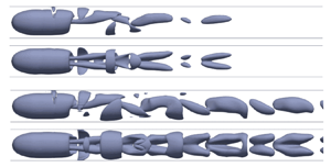
The temporal evolution of the wake for different Reynolds number and for a fixed area ratio are now analysed with DNS. Figure 19 displays the Q-criterion for the four Reynolds numbers $Re=130, 145, 175, 200$, with two plots for each case corresponding to the view in two orthogonal directions.

Figure 19.

Iso-contour of Q-criterion for $a/A=0.39$, two perpendicular views are represented for each case. From top to bottom, $Re=130, 145, 175, 200$.

For $Re=130$ (figure 19a), the flow corresponds to the axially symmetric state, in accordance with the LSA prediction. The wake is axially symmetric and the view is identical in both orthogonal directions. The structure behind the blunt body is stationary and it consists of a toroidal recirculation bubble. For $Re = 160$ (figure 19b), the $SS1$ steady, non-axisymmetric state is observed. The loss of axisymmetry results in a tilting of the toroidal structure attached to the body, the latter expanding in one direction and retracting in the opposite one.

The next states for $Re=175$ and $Re=200$ (figure 19c,d) correspond to the RSP oscillatory state. The toroidal recirculation gets destabilized and hairpin vortices are periodically advected in the streamwise direction. The interaction between those vortices and the wall is visible through wall shaped vortices which merge with the hairpin vortices as they move downstream.

Up to here, the sequence of bifurcations and the structure of the observed states are identical to the unconfined case (Bohorquez et al. Reference Bohorquez, Sanmiguel-Rojas, Sevilla, Jiménez-González and Martínez-Bazán2011; Bury & Jardin Reference Bury and Jardin2012). The main difference is that due to confinement, the bifurcations arise at a much lower Reynolds number value. For instance, Bohorquez et al. (Reference Bohorquez, Sanmiguel-Rojas, Sevilla, Jiménez-González and Martínez-Bazán2011) report the first bifurcation for $Re = 319$ and the second for $Re =413$.

Figure 20 displays the time history of the lift and drag coefficients (noted $C_\ell$ and $C_d$) characterising forces exerted on the body calculated from DNS, again for $a/A=0.39$.

Figure 20.

Lift and drag coefficients from DNS simulations ($L/d=2$ and $a/A=0.39$) vs dimensionless time, for (a) $Re=145$, (b) $Re=160$, (c) $Re=175$ and (d) $Re=200$.

For $Re = 130$ (case not displayed), the lift converges to a zero value. For all other cases, after a short transient (not shown), the simulations first seem to converge towards a steady state with zero lift, approximately in the range $t \in [30\unicode{x2013}50]$. The later evolution shows however that this state is not stable, and a phase of linear instability characterised by exponential growth of both coefficients is seen. In this linear phase the observed behaviour of the lift coefficient corresponds to a purely exponential growth with non-oscillating behaviour ($\approx e^{\sigma t}$ with real $\sigma$). This is a clear signature of the emergence of the non-oscillating mode $S1$ which is effectively the only unstable one detected by LSA for the values of considered $Re$.

For $Re=145$ (figure 20a) and for $Re = 160$ (figure 20b), the subsequent nonlinear evolution is a saturation towards the $SS1$ steady state with non-zero lift. On the other hand, for $Re=175$ (figure 20c), this steady state seems to be transiently approached by the solution, but then a second phase of linear instability follows, this time with oscillating behaviour ($\approx {\rm e}^{\sigma t}$ with complex $\sigma$) is observed. This trend is the signature of the existence of a non-oscillating mode related to the $O1$ mode. For $Re = 175$, the saturated state ultimately observed is the periodic, RSP state characterised by a lift force oscillating around a non-zero mean value. For $Re=200$ (figure 20d), the initial behaviour and ultimate state are similar, but transient towards the RSP state and displays a low-frequency modulation which is eventually damped.

The dimensionless frequency spectra of the two oscillating cases are presented in figure 21. They are performed from the $C_\ell$ signal of figure 20 and the transitional behaviours have been excluded. It has been verified that the sample is large enough and does not influence the spectra. Both spectra lead to similar observations. The two peaks can be interpreted as a fundamental frequency mode and its first harmonic. The amplitude of the first harmonic is much lower than the fundamental and, therefore, it is not visible to the naked eye on the signal which is very close to a pure sinusoid. As shown in the table found in figure 21(c), the influence of the Reynolds number on the Strouhal number $St$ is weak with this $Re$ range, DNS give a $2\,\%$ variation between $Re=175$ and $200$. This behaviour is substantiated by the quasi-constant $St$ values found using the LSA for low confinement (see figure 4b). The $St$ values given by DNS and LSA approaches are comparable even if a $16\,\%$ relative difference is measured between DNS ($Re=200$) and LSA at the threshold ($Re=201.2$). The discrepancy between these results can be explained by the fact that the $O1$ mode is obtained using an axially symmetric base flow whereas this base flow is no longer present in the DNS for $Re \geqslant 175$, the RSP state oscillates around steady state which is non-axisymmetric.

Figure 21.

Frequency spectra for DNS case $L/d=2$, $a/A=0.39$, $Re=175$ (a), $Re=200$ (b) and table of $St$ values of the higher peaks (DNS) with corresponding $St_c$ for LSA (c).

4.3. Towards nonlinear behaviours, moderately confined cases ($a/A=0.6$ and $0.74$)

Consider, now, the flow structures revealed by DNS in the range of moderately confined cases. The beginning of the bifurcation sequence is the same as described in the previous paragraph. With an initially symmetric state, followed by a steady, non-axisymmetric state. Figure 22(a,b) displays these two states observed respectively for $a/A = 0.74$; $Re = 100$ and $a/A = 0.74$; $Re = 115$. Similar structures are obtained for $a/A =0.6$ and the same values of $Re$ and are not displayed.

Figure 22.

Iso-contour of Q-criterion for moderately confined cases; two perpendicular views are represented for each case: (a) $a/A =0.74$, $Re=100$; (b) $a/A =0.74$, $Re=115$; (c) $a/A =0.74$, $Re=160$. For the last case, instantaneous representations for three different instants are displayed.

When raising the Reynolds number to $Re = 150$ in this range of moderately confined cases, nonlinearities lead to richer dynamics compared with the previous cases. Consider, first, the flow obtained for $a/A=0.74$ (figure 22c). Although the flow symmetries still indicate the (RSP) oscillatory state, the flow has a more complex structure than previously observed. Two main oscillating regions can be seen: the first one is the upper part of toroidal recirculation, close to the body, where a separated structure periodically appears. The second one is formed by a more distant structure, a $45^\circ$-inclined protrusion which is advected downstream. Sticking to the case $a/A=0.74$, $Re = 150$, figure 23(a) displays the time history of the lift and drag coefficients. The lift force shows a temporal modulation where both a low-frequency component (with dimensionless period of order 7.5) and a high-frequency component (with a period about 10 times shorter) can be discerned. The drag coefficient displays similar patterns but the amplitude of oscillations are extremely small (less than $0,5\,\%$ of the average value).

Figure 23.

Characterisation of time-dependent forces exerted on the body for $Re=150$, $a/A=0.74$: (a) time history of lift and drag coefficients, and (b) frequency spectrum of the lift coefficient.

Although the time series may suggest a quasi-periodic behaviour, analysis of the Fourier transform of the lift force (figure 23b) indicates that the behaviour is actually strictly periodic, as demonstrated by the existence of a fundamental frequency, $St_1=0.1308$ along with its harmonics. The spectrum also shows that apart form the fundamental, a high-frequency content is centred around the harmonic number $10$, corresponding to $St_{10}=1.308$. This matches with the high-frequency component detected in the time series with a period about $10$ times shorter compared with the low-frequency component.

Trying to relate these dynamics to the LSA results is a bit puzzling; going back to figure 13 shows that no unsteady modes exist for $a/A=0.74$ since $O1$ and $O2$ are only detected for $a/A < 0.73$ and the low-frequency $O3$ mode only arises for $a/A>0.75$. However, again, the results obtained from LSA considering the axisymmmetric base flow are only indicative here since the bifurcations arise from the steady non-axisymmetric state. The order of magnitude of the Strouhal number $St_1$ characterising the low-frequency oscillation is in the same range as the $O3$ mode which exists for $St \approx 0.1\unicode{x2013}0.2$, suggesting that the $O3$ mode actually plays a role in the nonlinear solution given by DNS.

Consider, now, the flow obtained for $a/A=0.6$ and $Re = 150$. The time series of the exerted forces (figure 24a) show that periodicity is clearly lost and indicate a chaotic behaviour. This is confirmed by examining the Fourier transform of the lift force (figure 24b) which now shows a broadband spectrum.

Figure 24.

Characterisation of time-dependent forces exerted on the body for $Re=150$, $a/A=0.6$: (a) time history of lift and drag coefficients, and (b) frequency spectrum of lift coefficient.

4.4. Towards nonlinear behaviours, high confinement flow at $a/A=0.85$

To end up the exploration of nonlinear dynamics, consider now a highly confined case with $a/A=0.81$. The first bifurcation again leads to the steady, non-axisymetric state and is well explained by the onset of mode $S1$. On the other hand, when raising the Reynolds number, the next bifurcation does not lead to time-dependent vortex shedding. Instead, the flow remains stationary, but it acquires a structure characterised by the shedding of six vortical structures compared with only two as in the $SS1$ state, as shown in figure 25(a) for $Re=150$. This structure is a strong indication of the presence of an eigenmode with azimuthal wavenumber $m=3$, and it is in accordance with the LSA results which indeed predict the existence of the steady mode $S3$ in the same range of parameters. Plotting the pressure in a transverse slice just behind the body in figure 25(b) indeed indicates a symmetry of order 3 (i.e. 3 symmetry planes). However, this symmetry is not perfect. Indeed, plotting the pressure in a slice located farther downstream in figure 25(c) rather demonstrates a symmetry of order one because the region of largest pressure (blue levels) is slightly displaced towards the left. The presence of a $m=1$ component in the flow also manifests by the existence of a non-zero lift force, as indicated by the time series in figure 26. This suggest that the observed flow structure actually results from the presence of both $S1$ and $S3$ modes.

Figure 25.

Illustration of the wake for $a/A=0.85$ and $Re=150$. Iso-contour of Q-criterion (a), side and rear diagonal views. Slices of the dimensionless pressure $p^*=p/(\rho U^2)$ in the wake of the body, at $x/D=1.2$ (b) and at $x/D=9$ (c).

Figure 26.

Lift and drag coefficient for DNS case $L/d=2$, $Re=150$ and $a/A=0.85$ vs dimensionless time.