2.1 Description of the procedure

In a general situation, the unsteady velocity field $\boldsymbol{u}(\boldsymbol{x},t)$ of a flow can be equivalently represented in the frequency domain by its Fourier modes $\hat{\boldsymbol{u}}(\boldsymbol{x},\unicode[STIX]{x1D714})$ . In the case of parallel flows, McKeon & Sharma (Reference McKeon and Sharma2010) demonstrated that $\hat{\boldsymbol{u}}(\boldsymbol{x},\unicode[STIX]{x1D714})$ is proportional to the dominant resolvent mode about the mean flow, given that the resolvent operator displays a clear separation of singular values. The more recent work of Beneddine et al. (Reference Beneddine, Sipp, Arnault, Dandois and Lesshafft2016) extended this result to non-parallel flows, and they showed that from a physical point of view, this separation relates to the existence of a strong instability mechanism. Therefore, for a flow displaying such an instability mechanism, this proportionality may be formalised, for instance in an axisymmetric framework and for the axial velocity component $u_{x}$ , as

with $\hat{u} _{x}$ the Fourier transform of the measured axial velocity, $\tilde{u} _{x}^{\unicode[STIX]{x1D714}}$ the axial velocity component of the dominant resolvent mode at the frequency $\unicode[STIX]{x1D714}$ and $\unicode[STIX]{x1D6EC}$ an unknown complex-valued function of $\unicode[STIX]{x1D714}$ , which we will refer to as the amplitude function. By assuming the knowledge of $\hat{u} _{x}$ at a given point $(x_{0},r_{0})$ , we obtain an evaluation of $\unicode[STIX]{x1D6EC}$ as

yielding the prediction of $\hat{u} _{x}$ at any point of the domain (with (2.1)). Note that $\unicode[STIX]{x1D6EC}$ may only be computed if both the resolvent mode and $\hat{u} _{x}$ are known at the point $(x_{0},r_{0})$ , which implies that this input point is within the domain where resolvent modes can be computed (i.e. where the mean flow is known).

Figure 1.

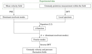
Graphical illustration of the reconstruction procedure.

In practice, the computation of the singular vectors of the resolvent operator requires knowledge of the mean flow over a wide region to correctly account for boundary conditions. Alternatively, for weakly non-parallel flows, one may use PSE analyses to obtain the dominant resolvent modes (see Beneddine et al. (Reference Beneddine, Sipp, Arnault, Dandois and Lesshafft2016)). This method, detailed in appendix A, does not require the definition of any streamwise boundary condition. It is therefore well suited to situations where the mean flow is measured over a relatively narrow region. Moreover, such a method has very low computational cost and does not require any advanced numerical algorithm. This motivated the use of PSE for the reconstruction presented here. The final procedure that we followed is graphically illustrated in figure 1. Note that the PSE technique cannot replace a resolvent analysis in any situation. For instance, as explained in Towne & Colonius (Reference Towne and Colonius2015), it is only adapted to behaviours involving a single right-going wave, and it may be unable to properly capture acoustic waves. In such a situation, a resolvent analysis is required to perform the reconstruction.

The previous explanations arbitrarily focus on the axial velocity for the description of the procedure. But the same relations hold for other flow quantities, and as shown by Beneddine et al. (Reference Beneddine, Sipp, Arnault, Dandois and Lesshafft2016), the resulting $\unicode[STIX]{x1D6EC}$ would not depend on which quantity is used. We could therefore use another velocity component, the pressure or any other quantity that is linearly dependent on these variables (such as the wall shear stress) to compute $\unicode[STIX]{x1D6EC}$ , and this $\unicode[STIX]{x1D6EC}$ may then be used to reconstruct all the flow quantities. This aspect is demonstrated in the case of the round jet studied here, in § 4.2 where both the radial velocity and the pressure fluctuation field are reconstructed from the sole knowledge of the axial velocity at one point.

Note that $\unicode[STIX]{x1D6EC}$ can be set equal to zero over some given frequency range, as this simply results in a frequency filtering of the reconstruction. This is useful for filtering out very low-energetic frequencies, and thus avoid non-useful computations. Indeed, the pointwise input measurement may have a rather high sampling frequency, such that its discrete Fourier transform (DFT) would be defined for a set of discrete values $\unicode[STIX]{x1D714}_{i}$ that would go up to very high values. Resolvent modes can be computed for every $\unicode[STIX]{x1D714}_{i}$ , but it is likely that a large number of them would have a very weak contribution to the dynamics (for instance the very high frequencies). Setting $\unicode[STIX]{x1D6EC}=0$ for these frequencies has a negligible impact on the final reconstruction.

Moreover, the reconstruction relies on the proportionality between Fourier and resolvent modes, which is expected for frequencies dominated by one strong convective instability mechanism (Beneddine et al. Reference Beneddine, Sipp, Arnault, Dandois and Lesshafft2016). The unsteadiness of the transitional jet studied in this paper entirely relates to the Kelvin–Helmholtz mechanism. As a result, the proportionality occurs for all energetic frequencies (see § 4.1), allowing an accurate unfiltered reconstruction. But in other situations, an instability mechanism may be dominant only for a limited frequency range $\unicode[STIX]{x1D6FA}$ : one may then set $\unicode[STIX]{x1D6EC}(\unicode[STIX]{x1D714})=0$ for $\unicode[STIX]{x1D714}\notin \unicode[STIX]{x1D6FA}$ and build an accurate filtered reconstruction within the frequency range $\unicode[STIX]{x1D6FA}$ .

It is important to stress that the present approach is applied here on a transitional jet. In the case of higher-Reynolds-number flows, it may fail to provide a full temporal reconstruction. In § 4.1, we will show that evaluating the Fourier modes by a DFT of the present experimental data at every point yields fields that are indeed proportional to the resolvent modes. This justifies that the reconstruction based on inverse DFT provides accurate results. Yet if the Reynolds number were significantly higher, the situation would be more complex. Indeed, Beneddine et al. (Reference Beneddine, Sipp, Arnault, Dandois and Lesshafft2016) showed that for highly turbulent flows, even when a large separation of singular values is observed, the resolvent modes are not proportional to the modes computed by DFT, but to the spatially correlated part of the fluctuation field, which may be obtained by a POD-based filtering. Since a simple inverse DFT of the POD-filtered spectrum would not yield the original (unfiltered) signal, the present approach may not straightforwardly reconstruct data in high-Reynolds-number turbulent flows. This is further discussed in the conclusion.

2.2 Causality of the reconstruction

In the present procedure, the time ranges of the reconstructed and input signals are the same, which raises the question of causality. This issue can be easily illustrated by considering a purely advective system, where a quantity (for instance the velocity $u$ ) at any time $t$ and at two streamwise locations $\boldsymbol{x}_{\mathbf{1}}$ and $\boldsymbol{x}_{\mathbf{2}}$ is such that $u(\boldsymbol{x}_{\mathbf{2}},t)=u(\boldsymbol{x}_{\mathbf{1}},t-\unicode[STIX]{x1D70F})$ , where $\unicode[STIX]{x1D70F}$ is a function of the convection velocity and the distance between the two points. In such a system, knowing $u(\boldsymbol{x}_{\mathbf{1}},t)$ for $t\in [0,t_{f}]$ is not enough to reconstruct $u(\boldsymbol{x}_{\mathbf{2}},t)$ over the same time interval. The reconstruction at $\boldsymbol{x}_{\mathbf{2}}$ would only be possible for $t\in [\unicode[STIX]{x1D70F},t_{f}+\unicode[STIX]{x1D70F}]$ . The missing part (i.e. for $t\in [0,\unicode[STIX]{x1D70F}]$ ) would require the knowledge of $u(\boldsymbol{x}_{\mathbf{1}},t)$ for $t\in [-\unicode[STIX]{x1D70F},0]$ .

In our approach, the reconstruction involves DFTs and inverse DFTs, which periodises the signals such that this missing past information ( $u(\boldsymbol{x}_{\mathbf{1}},t)$ for $t\in [-\unicode[STIX]{x1D70F},0]$ ) comes from $u(\boldsymbol{x}_{\mathbf{1}},t)$ for $t\in [t_{f}-\unicode[STIX]{x1D70F},t_{f}]$ . As a result, the present method violates causality by using future information to reconstruct past information. A limited part of the reconstruction, close to the borders of the reconstructed time interval, is therefore non-causal.

As shown in the next sections, the reconstruction is nonetheless satisfactory for the whole time range $[0,t_{f}]$ . This is due to the nature of the studied system, which is not purely advective but is characterised (in the frequency range of interest) by organised spatio-temporal large-scale structures, which allows one to determine (up to a certain limit) information pertaining to $t<0$ from information stemming from $t>0$ .

3.1 Experimental set-up and data processing

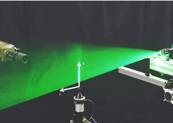
The experimental configuration studied in the present work (see figure 2) corresponds to that of Yegavian et al. (Reference Yegavian, Leclaire, Champagnat, Illoul and Losfeld2016). We have focused on a cold round jet at a Reynolds number $Re\approx 3300$ (based on the exit diameter of the nozzle $D=12~\text{mm}$ , the jet exit velocity $U_{e}=4.0~\text{m}~\text{s}^{-1}$ and the air viscosity at $T=15\,^{\circ }\text{C}$ ). From now on, all quantities are made non-dimensional by using $U_{e}$ and $D$ . The flow dynamics has been characterised in a diametral plane of the jet by TR-PIV measurements, using the experimental set-up and parameters presented in Yegavian et al. (Reference Yegavian, Leclaire, Champagnat, Illoul and Losfeld2016). Note that the coincidence of the laser sheet with a diametral plane has been ensured using precision devices, such that these planes can be considered nearly perfectly parallel (to within $3\times 10^{-3}$ radians) and separated by less than $9\times 10^{-3}$ non-dimensional length units.

Figure 2.

Picture of the experimental set-up, displaying the round jet, the high-speed laser and the camera. In the laser sheet plane, the streamwise direction is denoted by $x$ and the cross-stream direction by  $y$ .

The velocity field was measured from 10 000 snapshots taken at a frequency of 10 kHz (corresponding to 30 snapshots per non-dimensional time unit). Particles were illuminated by a 2 mm thick laser sheet using a Litron LDY303HE laser that provides an energy of 5 mJ per pulse. The snapshots have been processed using the FOLKI-PIV software, based on a classical two-frame estimation technique (Champagnat et al. Reference Champagnat, Plyer, Le Besnerais, Leclaire, Davoust and Le Sant2011). We used Gaussian interrogation windows of 19 $\times$ 19 pixels (corresponding to a size of 0.09 $\times$ 0.09 in non-dimensional units) with a standard deviation $\unicode[STIX]{x1D70E}=4$ pixels. Given the seeding density of our set-up (approximately 0.05 particle per pixel), the choice of this interrogation window size yields a good trade-off between noise and spatial resolution, in particular for the computation of the mean flow required for our reconstruction technique. This is further discussed in § 5.3. Note that such a seeding density is, however, low for planar PIV, and thus yields noisy instantaneous velocity fields with the classical two-frame approach. However, Yegavian et al. (Reference Yegavian, Leclaire, Champagnat, Illoul and Losfeld2016) showed that an accurate estimation may be obtained in these conditions when using the Lucas–Kanade fluid trajectory (LKFT) algorithm described in their paper, similar to other advanced time-resolved algorithms such as the fluid trajectory correlation technique (Lynch & Scarano Reference Lynch and Scarano2013) or fluid trajectory evaluation based on an ensemble-averaged cross-correlation (Jeon et al. 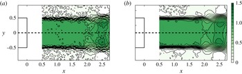Reference Jeon, Chatellier and David2014). Figure 3 compares snapshots obtained with the two approaches, and the noise indeed appears strongly reduced when using this alternative PIV processing.

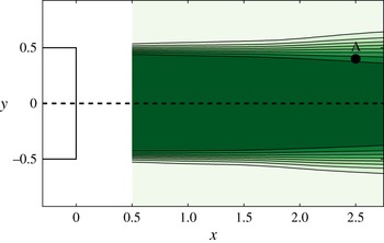
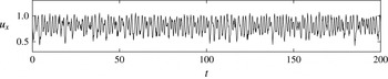
We therefore have two sets of velocity estimations for the present study. The two-frame noisy fields were used for the reconstruction procedure, both for computation of the mean flow (figure 4) and for extracting the local input signal necessary for the reconstruction (figure 5). On the other hand, the LKFT snapshots were used as a comparison to evaluate the quality of the reconstruction. In the following, we will refer to these sets of snapshots as the reconstruction set and the reference set, respectively. Using such a reconstruction set shows that the procedure is rather robust even in suboptimal experimental conditions. Moreover, to our knowledge, the experimental studies based on stability theory seldom use raw PIV results. For instance, the PSE analysis performed by Gudmundsson & Colonius (Reference Gudmundsson and Colonius2011) uses a mean flow computed from a Gaussian fitting of PIV measurements. As demonstrated in the next sections, the present approach may be successfully used without any fitting of the data acquired from classical measurement techniques, standard algorithms and a rather poor experimental set-up.

Figure 3.

Comparison between the instantaneous streamwise velocity field at $t=50$ obtained from (a) classical two-frame processing and (b) the LKFT algorithm. Velocities are non-dimensionalised using the jet exit velocity. The pointwise measurement and mean flow used in the reconstruction will be extracted or computed from the classical processing, and will therefore be referred to as the ‘reconstruction set’. The LKFT processing will be considered as the objective to attain, i.e. the ‘reference set’. The nozzle position (schematically represented in the panels) has been used to set the origin of the reference frame.

Figure 4.

Mean streamwise velocity field, computed from the reconstruction set of snapshots. Point A $(x_{0}=2.5,y_{0}=0.4)$ corresponds to the location where the unsteady signal used for the reconstruction has been extracted (also extracted from the reconstruction set). The nozzle position (schematically represented on the left of the figure) has been used to set the origin of the reference frame. The figure displays ten equally spaced contours ranging from 0 to 1.

Figure 5.

Streamwise velocity at point A $(x_{0}=2.5,y_{0}=0.4)$ versus time, extracted from the reconstruction set. The reconstruction presented in § 4.2 was done solely based on this signal and the mean flow shown in figure 4.

3.2 Characterisation of the unsteady behaviour of the jet

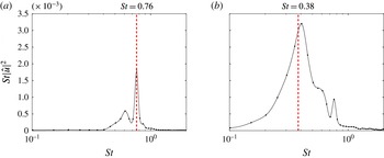
The unsteady behaviour of the jet near field can be qualitatively observed in both figures 3 and 6, where we see typical oscillations in the shear layer due to the Kelvin–Helmholtz instability mechanism. A quantitative characterisation of the dynamics has been made by computing frequency spectra at several locations in the jet from the reference velocity field. To obtain statistically converged spectra, the temporal velocity signals were processed following the classical Welch’s algorithm: the time series were divided into 49 bins of 600 snapshots with a 66 % overlap, the final spectra being obtained by averaging the spectra of each bin. Close to the nozzle, they display a clear peak around a Strouhal number $St=0.76$ (see figure 7 a). The boundary layer momentum thickness near the nozzle was measured as $\unicode[STIX]{x1D703}\approx 0.023$ , and therefore the Strouhal number based on $\unicode[STIX]{x1D703}$ is approximately 0.009, which is consistent with the existing work in the literature for low-Reynolds-number jets (see for instance Gutmark & Ho (Reference Gutmark and Ho1983)). At later stages of the development of the shear layer, the spectra become more broadband, and the energy shifts to lower frequencies. The dominant frequency becomes close to $St=0.38$ , corresponding to a subharmonic of the Kelvin–Helmholtz frequency (see figure 7 b). This can be attributed to downstream vortex pairing, as explained in Yegavian et al. (Reference Yegavian, Leclaire, Champagnat, Illoul and Losfeld2016).

Figure 6.

Instantaneous fluctuation field about the mean flow for an arbitrary time $t=50$ of (a) the streamwise velocity and (b) the cross-stream velocity (reference set). The streamwise velocity is symmetric with respect to $y=0$ while the cross-stream velocity is antisymmetric, as expected from a round jet, known to be dominated by axisymmetric fluctuations.

Figure 7.

Frequency spectrum of the streamwise velocity at (a) $x=1.0$ , $y=0.3$ and (b) $x=1.5$ , $y=0.25$ , computed from the PIV results (reference set). The upstream spectrum (a) displays a clear peak at $St=0.76$ , linked to the Kelvin–Helmholtz mechanism, while further downstream (b) displays a broader spectrum centred around $St=0.38$ . This latter frequency is related to the typical downstream vortex pairing that occurs in such flows.

The global dynamics of round jets is known to be dominated by fluctuation modes of azimuthal wavenumbers $m=0$ and $m=1$ , the $m=0$ mode being dominant where the shear layer thickness is small with respect to the diameter (see for instance Davoust, Jacquin & Leclaire (Reference Davoust, Jacquin and Leclaire2012)). In the present article, the investigated jet is measured rather near to the nozzle exit, and $\unicode[STIX]{x1D703}$ is approximately 0.023 near the nozzle, explaining the apparent axisymmetry of the fluctuations that can be clearly observed in the PIV snapshots (symmetric streamwise velocity field and antisymmetric cross-stream velocity field; see figure 6). Consequently, for the reconstruction procedure used in the rest of the study, we consider an axisymmetric framework, which has been validated a posteriori by the agreement between the PIV results and the axisymmetric PSE analysis (§ 4.1).

The axisymmetric assumption requires one to post-process the PIV velocity fields in order to accurately determine the streamwise direction and the location of the symmetry axis of the jet. To this end, the camera was carefully oriented to be approximately aligned with this axis. The small remaining misalignment was corrected by computing, for each streamwise location $x_{0}$ , the centre $y_{c}(x_{0})$ of the corresponding mean streamwise velocity profile $\overline{u}(x_{0},y)$ , defined as

The jet axis was computed by linear regression over the computed points $y_{c}$ , and then the velocity components were corrected with respect to this new orientation. Finally, the symmetry of the field with respect to this computed axis was assessed by evaluating the quantity

This relative measure of the symmetry of the jet was found to equal $0.039$ . This low value ensures the relevancy of the axisymmetric assumption. The origin of the new system of coordinates is chosen to be at the centre of the nozzle exit. Figure 4 presents the mean streamwise velocity field in this new frame of reference. Note that since the new fields are slightly rotated with respect to the original PIV snapshots, the discrete velocity values have been evaluated on a new grid centred around the axis of the jet using a third-order spline interpolation. The new grid covers the domain ( $0.5\leqslant x\leqslant 2.75$ , $-1\leqslant y\leqslant 1$ ) and contains 225 and 200 points in the streamwise and cross-stream directions, respectively. The effect of this interpolation has been assessed by considering a grid twice as dense in every direction. The impact on the snapshots, the mean field and the PSE results has been found to be weak.

4.1 Prediction of the Fourier modes from the mean flow

In this section, we aim to predict, for any arbitrary frequency $\unicode[STIX]{x1D714}_{0}$ , the spatial structure of the velocity Fourier mode $\hat{\boldsymbol{U}}(\boldsymbol{x},\unicode[STIX]{x1D714}_{0})$ from the sole knowledge of the mean flow, computed by time averaging the reconstruction set of PIV snapshots. As explained in § 2.1, this may be achieved by computing the dominant resolvent modes with a PSE analysis, by following the procedure detailed in appendix A. Note that the PSE analysis has been performed in an axisymmetric framework, using the axisymmetric mean flow defined by the upper half of the complete two-dimensional PIV mean flow (see figure 4). In the following, we therefore switch from Cartesian coordinates $(x,y)$ to cylindrical coordinates $(x,r)$ , and the axial and radial velocity, denoted by $u_{x}$ and $u_{r}$ , are taken equal to the streamwise velocity component $u$ and the cross-stream velocity component $v$ of the upper half of the PIV domain, respectively. One may alternatively use the lower half of the domain (but $u_{r}$ has to be taken equal to $-v$ ), but in our case, this second choice led to similar results, and therefore is not presented here. Note that in such an axisymmetric configuration, it is also possible to use both the upper and lower parts of the domain, which virtually gives twice as many snapshots to produce a mean flow that would be better converged. This may be useful when the number of available snapshots is rather low, but this was not the case for the present study, explaining why we did not use such processing.

Figure 8.

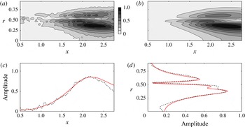
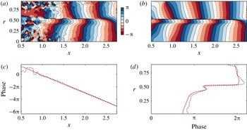
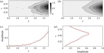
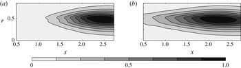
Comparison of the normalised modulus of the axial velocity of (a) the Fourier mode computed by a DFT of the reference TR-PIV measurements and (b) the dominant resolvent mode computed from the experimental mean flow only ( $St=0.76$ ). Panels (c,d) compare profiles from the Fourier mode (dashed line) and the dominant resolvent mode (continuous red line), extracted at $r=0.4$ and $x=2.0$ , respectively.

Figure 9.

Comparison of the normalised phase of the axial velocity of (a) the Fourier mode computed by a DFT of the TR-PIV measurements and (b) the dominant resolvent mode computed from the experimental mean flow only ( $St=0.76$ ). Panels (c,d) compare profiles from the Fourier mode (dashed line) and the dominant resolvent mode (continuous red line), extracted at $r=0.4$ and $x=2$ , respectively. The phase profiles have been unwrapped.

Figure 10.

Comparison of the normalised modulus of the radial velocity of (a) the Fourier mode computed by a DFT of the TR-PIV measurements and (b) the dominant resolvent mode computed from the experimental mean flow ( $St=0.38$ ). Panels (c,d) compare profiles from the Fourier mode (dashed line) and the dominant resolvent mode (continuous red line), extracted at $r=0.5$ and $x=2.5$ , respectively.

Figure 11.

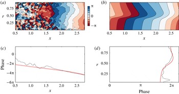
Comparison of the normalised phase of the radial velocity of (a) the Fourier mode computed by a DFT of the reference TR-PIV measurements and (b) the dominant resolvent mode computed from the experimental mean flow ( $St=0.38$ ). Panels (c,d) compare profiles from the Fourier mode (dashed line) and the dominant resolvent mode (continuous red line), extracted at $r=0.5$ and $x=2.5$ , respectively. The phase profiles have been unwrapped.

The Fourier modes were computed by a DFT of the reference set of PIV snapshots. Figures 8 and 9 assess the proportionality of the axial velocity of the dominant resolvent mode and the Fourier mode (modulus and phase comparison of the fields, respectively), for $St=0.76$ (the Kelvin–Helmholtz frequency; see § 3). Figures 10 and 11 show the same comparison for the radial velocity, for $St=0.38$ (the Kelvin–Helmholtz subharmonic). For the sake of comparison, the modulus of every mode has been normalised such that its maximum is 1, and the phases such that they are equal to zero at an arbitrary location $x=2.25$ , $r=0.3$ . These figures illustrate for the two velocity components, and for two different characteristic frequencies of the flow, that, as claimed in § 2.1, the dominant resolvent mode is approximately proportional to the Fourier mode (their moduli are approximately equal up to a multiplicative constant and their phases up to an additive constant). However, this agreement strongly deteriorates in low-energy parts of the flow. This is particularly striking in figure 11 for instance. We see that close to $r=0$ , as well as for $x<1.7$ , the two fields show a strong discrepancy. While it is known that the dominant modes may not reproduce well the actual dynamics in the low-energy parts of the flow (see Beneddine et al. (Reference Beneddine, Sipp, Arnault, Dandois and Lesshafft2016)), here the discrepancy could also be attributed to the difficulty of measuring a signal with such a low fluctuating energy. Fluctuations in these regions are instead dominated by measurement noise, which does not allow any relevant comparison. Similar overall agreement has been found for all the other investigated frequencies, for both the axial and radial velocity components. This agreement justifies a posteriori the validity of the axisymmetric hypothesis.

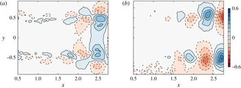
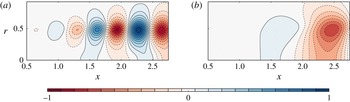
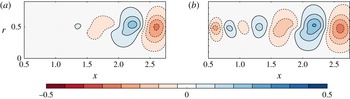
The PSE analysis also yields the prediction of the pressure modes, for which we do not have any experimental comparison. Figure 12 presents the real part of the pressure mode for the Kelvin–Helmholtz frequency $St=0.76$ and the subharmonic $St=0.38$ , where one can see alternating positive and negative pressure regions along the shear layer, as classically observed in shear layers. We also observe that the downstream structure that appears in figure 12(b) is approximately twice as large as the structures in figure 12(a), consistent with the assumption that the frequency $St=0.38$ is related to downstream vortex pairing.

Figure 12.

Real part of the pressure Fourier mode computed with the PSE analysis, from the experimental mean velocity field for (a) $St=0.76$ and (b) $St=0.38$ , corresponding respectively to the Kelvin–Helmholtz frequency and its subharmonic. The downstream structure of panel (b) is approximately twice as large as the structures of panel (a), consistent with the fact that this Kelvin–Helmholtz subharmonic is related to downstream vortex pairing.

4.2 Time-resolved reconstruction of the snapshots

Following the procedure of § 2.1, we computed the amplitude function $\unicode[STIX]{x1D6EC}$ using the axial velocity $u_{x}$ at $x_{0}=2.5$ , $r_{0}=0.4$ (the input signal can be seen in figure 5). This choice of input point is discussed in more detail in § 5.1. The choice of the axial velocity as the input quantity was arbitrary; using the radial velocity led to similar results (not presented here). The snapshots are finally reconstructed by performing an inverse DFT at every spatial point. The $\unicode[STIX]{x1D6EC}$ function was computed for $0.2<St<1.4$ , which contains most of the energy of the flow (see figure 7), following relation (2.2). Outside of this range, we set $\unicode[STIX]{x1D6EC}=0$ , which filters the low-energy part of the spectra. In this frequency range, we computed 400 resolvent modes. This number stems from the frequency resolution of the DFT of the input signal, a mode being computed for every frequency within the range considered. Note that the final reconstructed set of snapshots has therefore the same time sampling and duration as the input signal used for the computation of $\unicode[STIX]{x1D6EC}$ .

Figure 13.

Comparison of the axial velocity of (a) the reconstructed field and (b) the TR-PIV field (reference set) at $t=75$ .

Figure 14.

Comparison of the axial velocity computed from the TR-PIV snapshots (reference set, dashed line) and the reconstructed signal (red continuous line) at $x=2.0$ and $r=0$ (a point presenting an intermediate level of energy), for an arbitrary time range $50<t<100$ .

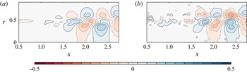
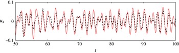
The reconstructed snapshots display good agreement with the reference set, as can be seen in figure 13, which compares an axial velocity snapshot with the reference PIV field. The size and location of energetic structures are well reconstructed. The agreement is also good in lesser-energy locations. This can be seen in figure 14, which compares the temporal evolution of the axial velocity from the reconstruction and the reference set at the point $(x=2.0,r=0)$ . The oscillations of both signals are well in phase, and their amplitude is very close. Note that the comparison cannot be made in very low-energy parts of the flow, such as the near-axis and most upstream zones in figure 11. This stems from the fact that the reference set is not accurate in such regions (the signal-to-noise ratio is low) and the model is not designed to reconstruct low-energy behaviour anyway (see Beneddine et al. (Reference Beneddine, Sipp, Arnault, Dandois and Lesshafft2016)).

In order to provide a more quantitative comparison, we introduce an instantaneous global measure of the error, denoted by $e(t)$ , defined as

with $N_{p}$ the number of discrete points where the velocity is known, and $u_{x}^{i}$ and $u_{x,0}^{i}$ the $i$ th discrete streamwise velocity values of the reconstructed field and of the reference field, respectively. This quantity corresponds to the root mean square over the whole domain of the velocity error, expressed in non-dimensional units. 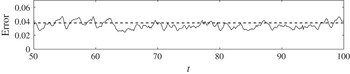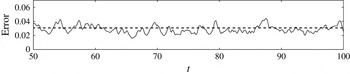One should note that both the reconstruction errors and the PIV measurement errors contribute to the value of $e(t)$ , therefore it would not be zero even in the case of a perfect reconstruction. Figure 15 shows the temporal evolution of this error, and we see that the discrepancy between the reference and the reconstruction does not vary much with time (approximately 0.04), ensuring that the global quality of the reconstruction is approximately constant over the full time range considered.

Figure 15.

Time evolution of the global axial velocity error (continuous line) for an arbitrary temporal range $50<t<100$ . The dashed line represents the mean error over the full time range ( $0<t<333$ ), which is approximately equal to 0.038.

Figure 16.

Comparison of the radial velocity of the reconstructed field (a) and the reference PIV fields (b) at $t=75$ .

Figure 17.

Time evolution of the global radial velocity error (continuous line) for an arbitrary temporal range $50<t<100$ . The dashed line represents the mean error over the full time range ( $0<t<333$ ), which is approximately equal to 0.031.

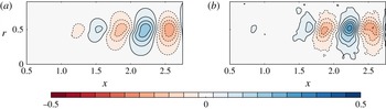
As explained in § 2.1, the amplitude function $\unicode[STIX]{x1D6EC}$ computed from only one flow variable (here the axial velocity) yields the reconstruction of all other fluctuating quantities (pressure and radial component of velocity). Figure 16 compares a reconstructed radial velocity snapshot with the corresponding reference field, and the agreement is once again favourable. Figure 17 shows the temporal evolution of $e$ , and the level of error is again rather steady over time, with values close to that of the axial velocity (approximately 0.03). For the pressure reconstruction, we do not have experimental results to serve as reference, but the accurate reconstruction of the radial velocity is a strong argument in favour of the quality of the pressure reconstruction. Indeed, nothing distinguishes these two variables in our approach. 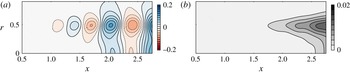Moreover, the resulting pressure fluctuation field $p^{\prime }(x,r)$ is reminiscent of what is expected in such a jet (see figure 18 a), with alternating positive and negative pressure regions that grow in size and amplitude when moving downstream.

Figure 18.

(a) Reconstructed pressure fluctuation field at $t=75$ ; (b) mean square pressure fluctuation field $\overline{p^{\prime 2}}$ .

Figure 19.

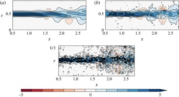
Comparison of the azimuthal vorticity at $t=75$ , computed from (a) the PSE-based reconstructed field, (b) the reference PIV set and (c) the reconstruction PIV set.

Another remarkable feature of the reconstructed fields is their smoothness, which makes them easily differentiable. This is of high importance for the computation of derived quantities such as the vorticity, which is sometimes difficult to accurately compute from PIV measurements, especially in a time-resolved context where the fields display stronger noise. As an illustration, figure 19 compares a vorticity snapshot computed from the PSE reconstruction, the reference PIV set and the reconstruction PIV set. The fields have been obtained from differentiation of the velocity snapshots, based on second-order centred finite differences, with a stencil length equal to 0.08 (twice the length of the interrogation window used for the PIV estimation). The reconstructed vorticity compares very favourably with the reference. The vorticity directly derived from the PIV reconstruction set illustrates the kind of results that are obtained from PIV when the level of noise is too high. This strongly deteriorates the estimation of the derivatives, while the same level of noise in the input data for the PSE reconstruction has no similar impact on the reconstructed field. Note that the vorticity is one among many other derived quantities that may be determined from the present reconstruction. For instance, figure 18(b) shows the mean square pressure fluctuation field $\overline{p^{\prime 2}}$ , and any mean square fluctuation or Reynolds stress term could be similarly computed, and exploited for further physical analysis.

5.1 Influence of the choice of input point

The reconstruction model of this work is based on that of Beneddine et al. (Reference Beneddine, Sipp, Arnault, Dandois and Lesshafft2016), who explained that the point used for the computation of the function $\unicode[STIX]{x1D6EC}$ should be in a high-energy region of the flow to yield an accurate reconstruction. This requirement stems from the fact that the dominant resolvent modes accurately reproduce the Fourier modes in these regions, but there is no guarantee that this agreement would be as good in low-energy regions. This is confirmed in our case, and can be seen in figures 8 to 11, where we see that the strongest discrepancy between dominant resolvent modes and Fourier modes appears in low-energy regions. But as mentioned in § 4.1, in our case this could be attributed to a poor signal-to-noise ratio in low-energy regions of the flow, a common problem in experimental studies. This issue can be clearly seen in figures 9(a) and 11(a) for instance, where the non-energetic upstream part of the domain has strong noise, yielding a significant discrepancy with the dominant resolvent fields.

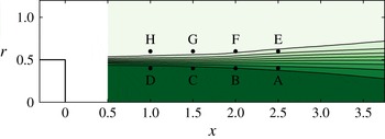
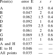
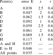
To assess the sensitivity of the results to the input point, we considered seven additional points along the shear layer for the determination of $\unicode[STIX]{x1D6EC}$ (in total, four points above the shear layer and four points below; see figure 20 for the position of the points). The reconstruction is based on the streamwise component of the velocity only, as was done in § 4.2. For each of these points, we computed the global error $E$ , defined as

with $T_{max}=333$ the duration of the TR-PIV acquisition and $e$ the instantaneous error (see (4.1)). The resulting values can be seen in table 1, and we observe two clear tendencies: the points located downstream yield a smaller error than the ones located upstream, and the points above the shear layer display a larger error than the ones below. This is fully consistent with the findings of Beneddine et al. (Reference Beneddine, Sipp, Arnault, Dandois and Lesshafft2016), who explained that input points located in high-energy regions yield smaller error. Indeed, here the downstream region contains more energy than the upstream one, where the Kelvin–Helmholtz instability has not fully developed yet. Also, concerning the axial velocity, the region inside the jet has been found to be more energetic than the region outside. This can be observed for instance in figure 8 for $St=0.76$ .

Figure 20.

Position of the eight points considered to study the influence of the input point location on the accuracy of the reconstruction; point A is the original point considered in § 4.2.

For a given flow configuration, the location of high-energy regions may usually be determined by prior physical knowledge of the qualitative dynamics of the flow. It may therefore be easy to predict good locations for the input sensor in most situations. However, it is likely that the flow dynamics would involve several characteristic frequencies, or even a range of frequencies, and that these frequencies would be related to different locations of the flow. In such a case, it is not possible to find a single location that would be energetic for all these frequencies. As explained by Beneddine et al. (Reference Beneddine, Sipp, Arnault, Dandois and Lesshafft2016), this may be treated by considering $n$ points for the determination of $\unicode[STIX]{x1D6EC}$ , leading to an overdetermined set of $n$ equations $\{\unicode[STIX]{x1D6EC}(\unicode[STIX]{x1D714})=\hat{u} _{x}(\unicode[STIX]{x1D714},x_{k},r_{k})/\tilde{u} _{x}^{\unicode[STIX]{x1D714}}(x_{k},r_{k}),1\leqslant k\leqslant n\}$ that may be solved by least squares. The resulting $\unicode[STIX]{x1D6EC}$ would be weakly affected by low-energy points, such that for every frequency, only high-energy points would contribute to its value. The reconstruction would also be likely to be more accurate because it would be based on more input data. Finally, multiplying the number of input points may be useful when there is not any prior knowledge of the energetic regions, or when this knowledge is not accurate enough, since only one of the sensors needs to be well positioned.

We have tested this approach by considering the best and worst points together (A and H; see table 1). The result, close to that obtained with A only, shows that the reconstruction is not degraded by the poorly chosen point H. Therefore, in an experimental context, an accurate prediction would be achieved by using several pointwise measurements as long as at least one of them is located in a high-energy part of the flow for each frequency of interest. We also tested the four points above the shear layer (E to H) together, as well as all points together, and table 1 shows that when $\unicode[STIX]{x1D6EC}$ is based on a set of points, the results appear to be always more accurate than the single-point reconstruction based on the best point of the set. This is of high importance in an experimental context, when using a sensor at some specific high-energy points may be too intrusive (for example at points A to D). This gives more flexibility to the method, since lower-energy points might also be used, as long as they are sufficiently numerous. In particular, one may position a rather large number of sensors downstream from the region of interest and obtain a satisfactory reconstruction, even if this region is not the most energetic one.

Table 1.

Comparison of the global error for different input points or sets of points.

5.2 Impacts of an inaccurate knowledge of the input sensor position

The present procedure is intended to be used with unsteady data obtained from pointwise sensors. However, in practice, the spatial positions of these sensors can be subject to some uncertainties. In this section, the impact of such inaccurate knowledge of an input sensor position on the quality of the unsteady reconstruction is studied by considering an input sensor positioned at $(x_{0}+\unicode[STIX]{x1D6FF}x,r_{0}+\unicode[STIX]{x1D6FF}r)$ , but which would be erroneously assumed to be located at $(x_{0},r_{0})$ . In the procedure, this amounts to selecting a different input signal from that of figure 5, such that the computed amplitude function is no longer defined by (2.2), but becomes equal to the following biased amplitude function:

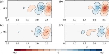
For the reconstruction, we found that such a misplacement mainly results in a streamwise translation of the structures of the fields and, to a lesser extent, a moderate change in their overall amplitude and shape. This overall effect on the reconstruction can be seen in figure 21 for $\unicode[STIX]{x1D6FF}x=\unicode[STIX]{x1D6FF}r=0.05$ , $\unicode[STIX]{x1D6FF}x=\unicode[STIX]{x1D6FF}r=0.1$ and $\unicode[STIX]{x1D6FF}x=\unicode[STIX]{x1D6FF}r=-0.2$ ( $\unicode[STIX]{x1D6EC}$ is computed from the axial velocity and $(x_{0},r_{0})=(2.5,0.4)$ ). In physical units, this corresponds respectively to misplacements of $0.85$ , $1.7$ and $3.4~\text{mm}$ , i.e. from realistic up to overestimated experimental positioning errors. When compared with an unbiased reference snapshot (figure 21 a), these biased snapshots seem to all present a phase shift. Besides this dephasing, the resulting field displays the expected physical features (alternating positive and negative structures along the shear layer that grow in size and amplitude in the streamwise direction). This demonstrates that despite a possibly significant misplacement, the reconstruction does not degenerate but rather keeps a certain physical relevancy. This may be explained by the fact that here we consider flows displaying coherent structures, which present by definition a strong spatial correlation. Therefore, the energy content of the frequency spectrum will not suddenly change upon considering a point that is slightly misplaced (the spectrum will display a similar shape with the same dominant frequencies). The phase of the spectrum may, however, change significantly, which explains why the main observable effect of a misplacement is a dephasing of the fields.

Figure 21.

Comparison of the streamwise velocity of (a) the unbiased reconstructed field (no misplacement of the input sensor), (b) biased reconstructed field with $\unicode[STIX]{x1D6FF}x=\unicode[STIX]{x1D6FF}r=0.05$ , (c) biased reconstructed field with $\unicode[STIX]{x1D6FF}x=\unicode[STIX]{x1D6FF}r=0.1$ and (d) biased reconstructed field with $\unicode[STIX]{x1D6FF}x=\unicode[STIX]{x1D6FF}r=-0.2$ , for $t=10$ and $(x_{0},r_{0})=(2.5,0.4)$ . The reconstruction is performed using the axial velocity component.

Despite this weak overall impact on the physical features of the reconstruction, it may still be interesting to minimise the sensitivity with respect to misplacements by a relevant choice of input data. To address this issue, let us decompose the biased amplitude function $\unicode[STIX]{x1D6EC}_{b}$ as

with $\unicode[STIX]{x1D6EC}=\hat{u} _{x}(\unicode[STIX]{x1D714},x_{0},r_{0})/\tilde{u} _{x}^{\unicode[STIX]{x1D714}}(x_{0},r_{0})$ the unbiased amplitude function defined by (2.2) and $\unicode[STIX]{x1D6FF}\unicode[STIX]{x1D6EC}$ a spurious term that reads

with $\unicode[STIX]{x1D6FF}\hat{u} _{x}=\hat{u} _{x}(\unicode[STIX]{x1D714},x_{0}+\unicode[STIX]{x1D6FF}x,r_{0}+\unicode[STIX]{x1D6FF}r)-\hat{u} _{x}(\unicode[STIX]{x1D714},x_{0},r_{0})$ . For the reconstruction to be weakly affected by the misplacement of the sensor, $\unicode[STIX]{x1D6FF}\unicode[STIX]{x1D6EC}$ has to be small with respect to $\unicode[STIX]{x1D6EC}$ , which would ensure that each Fourier mode is rebuilt with good accuracy. The spurious effect of the misplacement may therefore be evaluated by the ratio $b=|\unicode[STIX]{x1D6FF}\unicode[STIX]{x1D6EC}/\unicode[STIX]{x1D6EC}|=|\unicode[STIX]{x1D6FF}\hat{u} _{x}/\hat{u} _{x}|$ . Finally, using the proportionality between the Fourier modes and the dominant resolvent modes yields the following expression for $b$ :

This expression only involves the dominant resolvent modes, and may therefore be computed by knowing only the mean flow. Assuming that the misplacement $(\unicode[STIX]{x1D6FF}x,\unicode[STIX]{x1D6FF}r)$ is small, $b$ may be linearised as

with $b_{x}$ and $b_{r}$ respectively the axial and radial sensitivity coefficients defined as

Small values of  $|b_{x}|$  and $|b_{r}|$  correspond to low sensitivity with respect to misplacements of the sensors, but the converse is not true, as $b$ may be small even for large values of $|b_{x}|$ and $|b_{r}|$ (errors along $x$ and $r$ may compensate for each other). In addition, the value of this coefficient does not give any indication regarding the type of effect of a misplacement, which could be a simple phase shift (as evidenced in figure 21), or a more significant distortion of the fields. Therefore, this coefficient only gives qualitative guidelines to minimise the impact of misplacements.

First, it should be noted that these coefficients depend on the input physical quantity considered: here $b_{x}$ and $b_{r}$ are defined from $u_{x}$ , but using for instance the radial velocity $u_{r}$ as input data for the reconstruction yields $b_{x}=\unicode[STIX]{x2202}_{x}\tilde{u} _{r}^{\unicode[STIX]{x1D714}}/\tilde{u} _{r}^{\unicode[STIX]{x1D714}}$ and $b_{r}=\unicode[STIX]{x2202}_{r}\tilde{u} _{r}^{\unicode[STIX]{x1D714}}/\tilde{u} _{r}^{\unicode[STIX]{x1D714}}$ . Consequently, the sensitivity with respect to misplacements may be reduced by considering an input physical quantity whose Fourier modes do not exhibit strong spatial gradients. In the case of the jet, while the axial velocity modes display some abrupt variations across the shear layer, as can be seen for instance in figure 9, the radial velocity or pressure modes do not display such high-gradient regions (see figures 10 and 12). The reconstruction may be more robust if based on a local record of one of these two quantities, especially if the sensors are designed to be near the shear layer.

Equations (5.6) and (5.7) also give insight into the best locations for the input sensors. Due to the division by the local amplitude of the resolvent modes in (5.7), $b_{x}$ and $b_{r}$ are expected to be small in high-energy regions, as long as the local spatial gradients do not become too strong. Moreover, the spatial gradients are expected to be rather small in the direct neighbourhood of a local energy maxima. 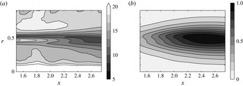Figure 22 compares the quantity $|b_{x}|+|b_{r}|$ (computed from the radial velocity modes) with $|\tilde{u} _{r}^{\unicode[STIX]{x1D714}}|$ for $St=0.76$ , and we see that high-energy regions are indeed rather weakly sensitive. While the considerations related to the sensor misplacements completely differ from those of § 5.1, we are here led to a similar conclusion: the input sensors should be preferably positioned in energetic regions.

Figure 22.

(a) Sensitivity map with respect to misplacements of the input sensors, for the radial velocity $u_{r}$ used an input (the quantity displayed is $|b_{x}|+|b_{r}|$ ); (b) radial velocity modulus of the normalised dominant resolvent mode. For both panels, $St=0.76$ . The panels show a relative correspondence between low-sensitivity and high-energy regions.

Finally, this rather good correspondence between high-energy and low-sensitivity points is interesting if multiple input points are considered for the computation of $\unicode[STIX]{x1D6EC}$ . The procedure used for the determination of $\unicode[STIX]{x1D6EC}$ is then based on a least-squares minimisation that rules out the low-energy points, for each single frequency of the reconstruction (see § 5.1). It is therefore expected to also rule out the high-sensitivity points, which increases the overall robustness of the method.

5.3 Sensitivity with respect to the mean flow measurements

The PIV measurements need to be accurate enough to yield a proper mean flow. In addition to the experimental conditions, the key parameter that influences the quality of the PIV velocity estimation is the size of the interrogation window: a large interrogation window contains more particles, which reduces the measurement noise, but it tends to smooth down the spatial gradients of the flow.

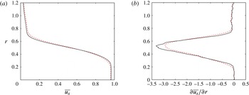
In the previous sections, we have used a mean flow that yields an accurate reconstruction, confirming a posteriori that the choice of the size of the interrogation windows was appropriate (see § 3). Choosing a smaller window increases the level of noise, but this does not have any significant impact on the final mean flow, as long as the number of snapshots used for the time averaging is high enough for convergence to be reached. However, taking an overly large interrogation window yields a mean flow that displays inaccurate, biased spatial gradients. This may be observed in figure 23, which compares the original mean flow (mean flow A) with a new mean flow (mean flow B), obtained with interrogation windows twice as large in each direction (Gaussian window, 37 $\times$ 37 pixels, $\unicode[STIX]{x1D70E}=8$ ). The overall effect of this enlargement is an underestimation of the spatial derivatives of the mean flow. For $St=0.38$ (the dominant frequency in the downstream zone of the flow), the dominant resolvent modes computed from mean flow A or B have been found to be hardly distinguishable. However, as we go to higher frequencies, an increasingly strong discrepancy appears when considering one mean flow or another. This discrepancy is therefore particularly important for high frequencies, as can be seen for instance in figure 24: for the Kelvin–Helmholtz frequency $St=0.76$ , the mode computed from mean flow B is abnormally energetic in the upstream region of the jet. The impact on the final reconstruction may be observed in figure 25 (reconstruction based on the axial velocity at ( $x=2.5$ , $r=0.4$ )): while the large low-frequency structures are correctly reconstructed downstream, some spurious high-frequency structures appear upstream of the flow.

These results show that the quality of the reconstruction is conditioned by the accuracy of the mean flow measurement, and one crucial aspect is the correct evaluation of the spatial gradients of the mean flow. In our case, it is found that when these gradients are erroneously evaluated, the final reconstruction exhibits abnormal levels of energy for high-frequency structures only. Note that this kind of preoccupation mainly concerns configurations where the seeding density would be particularly low, or where some parts of the flow contain really few particles. These two situations would be the only ones justifying the use of windows so large that it would have a significant impact on the PSE analysis.

Figure 23.

Comparison between mean flow A (black continuous line) and mean flow B (red dashed line), the latter corresponding to a PIV processing with a larger interrogation window. Panels (a) and (b) respectively display $\overline{u_{x}}$ and $\unicode[STIX]{x2202}\overline{u_{x}}/\unicode[STIX]{x2202}r$ at $x=2$ , where $\overline{u_{x}}$ is the mean axial velocity.

Figure 24.

Comparison between the normalised modulus of the dominant resolvent mode (radial velocity) at $St=0.76$ computed from (a) mean flow A (reference mean flow) and (b) mean flow B (larger interrogation window in the PIV processing).

Figure 25.

Comparison between a reconstructed radial velocity snapshot computed from (a) mean flow A (reference mean flow) and (b) mean flow B (larger interrogation window in the PIV processing).