1. Introduction
Acoustic liners are widely used in aeroengines to control noise emissions from inlet and bypass flow ducts (Tester Reference Tester1973; Rienstra & Eversman Reference Rienstra and Eversman2001; Rienstra & Darau Reference Rienstra and Darau2011). A couple of rigid strips are normally used to clamp lining surfaces over an otherwise rigid inner duct wall (Regan & Eaton Reference Regan and Eaton1999). These axially running strips, which are formally known as splices, excite acoustic scattering of different circumferential modes (Bi et al. Reference Bi, Pagneux, Lafarge and Aurégan2007), some of which are prone to cut-on and could eventually compromise acoustic performance. It is important to clarify the acoustic impacts of rigid splices in the presence of flows, although spliceless lining surfaces just become possible for some of the most recent inlet designs. Until now, the influence of splices has mainly been examined in terms of induced spinning modes with respect to their numbers and width in the circumferential axis, using either numerical simulations (McAlpine & Wright Reference McAlpine and Wright2006; Tam, Ju & Chien Reference Tam, Ju and Chien2008) or analytical methods, such as mode matching (Fuller Reference Fuller1984; Elnady, Boden & Glav Reference Elnady, Boden and Glav2001; Yang & Wang Reference Yang and Wang2008), multi-modal method (Bi et al. Reference Bi, Pagneux, Lafarge and Aurégan2006), Green’s function approach (Brambley Reference Brambley2009) and eigenmode analysis (Fuller Reference Fuller1984; Brambley, Davis & Peake Reference Brambley, Davis and Peake2012). We should say that the above literature review is not exhaustive. However, to the best of our knowledge, a theoretical model that illuminates scattering from hard–soft interfaces in both axial and circumferential directions is still not available. Hence, here we incorporate Fourier series expansion and the Wiener–Hopf method together to develop this theoretical model, which is the main contribution of this work.
The Wiener–Hopf method is a classical mathematical tool that could yield closed-form analytical solutions for scattering problems (Noble Reference Noble1958). Munt (Reference Munt1977), amongst others, applied this method to predict far-field directivity patterns of spinning modal radiations from cylindrical rigid ducts with jet flows. Rienstra (Reference Rienstra1984, Reference Rienstra2003b , Reference Rienstra2007) extended this study to a semi-infinite lined cylindrical duct along with the provision of a comprehensive analysis. Gabard & Astley (Reference Gabard and Astley2006) gave a thorough theoretical development for annular duct cases. Veitch & Peake (Reference Veitch and Peake2008) elegantly demonstrated the matrix Wiener–Hopf method for coaxial duct cases with staggered open ends. All these works gradually enhanced the theoretical modelling capability for progressively complicated set-ups of practical importance, but still only considered an impedance discontinuity in the axial direction. The variance in the circumferential direction was not studied previously by using the Wiener–Hopf technique. To address this issue, our work endeavours to develop a theoretical model to enable the analytical study of liner splices in flow ducts.
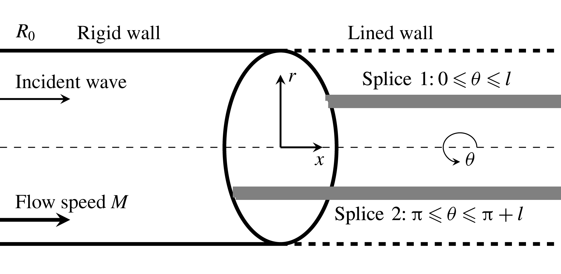
Sketch of the model problem in cylindrical coordinates
 $(x,r,{\it\theta})$
. The
 $x$
coordinate is aligned with the centre axis and is parallel to the walls. The
 $r$
direction is normal with respect to the walls at
 $r=\pm R_{0}$
. The left half semi-infinite wall (
 $x<0$
) is rigid and the right half semi-infinite wall (
 $x>0$
) is lined except for the
 $N$
axial rigid splices (grey lines, here
 $N=2$
). Here
 $l$
denotes the width of the splices in the
 ${\it\theta}$
direction. The background flow is presumably uniform with a normalised speed
 $M$
.
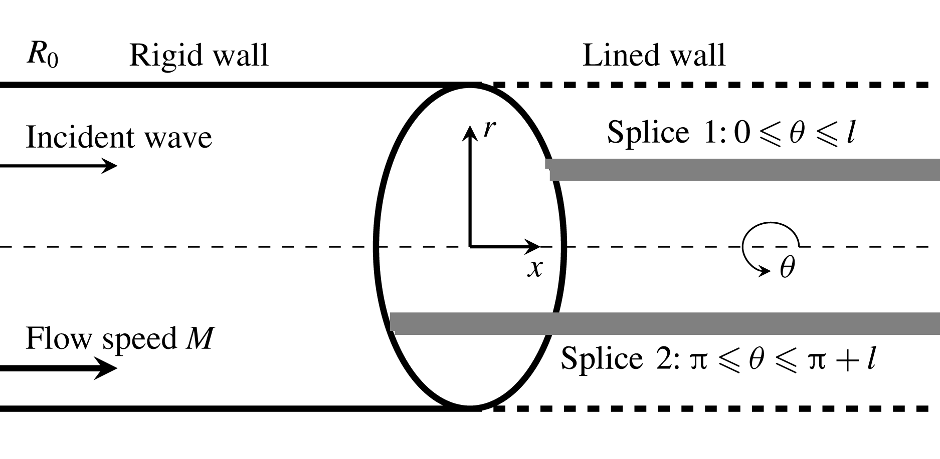
As shown in figure 1, the problem considered in this work contains impedance discontinuities in both axial and circumferential directions. The semi-infinite lining surface is covered by a couple of semi-infinite, axially running splices, which are equally spaced in the circumferential direction. Similar geometrical set-ups with either finite length (Regan & Eaton Reference Regan and Eaton1999; Duta & Giles Reference Duta and Giles2006) or infinite length for splices (Yang & Wang Reference Yang and Wang2008) can be found in previous works. Spinning modal waves incident from fan-stator assemblies (which are not shown here) will propagate inside the duct and impinge on the lining surface and rigid splices. The problem is described in the cylindrical coordinate system. The remaining part of this paper is organised as follows. We will first develop the theoretical model in § 2 to study scattering waves from this semi-infinite lining surface with rigid splices by incorporating the Wiener–Hopf method and Fourier series. Then, numerical cases will be conducted to validate the proposed theoretical model, and more associated results will be discussed in § 3. Finally, § 4 will summarise the present work.
2. The theoretical model
2.1. Statement of the problem
Here we study acoustic perturbations in a lined duct that contains a uniform mean flow. Boundary layer and vorticity are omitted to enable the follow-up theoretical developments with the Wiener–Hopf technique. If we assume much larger time scale and length scale of fluid dynamics than the corresponding scales of acoustic waves, sound propagation and scattering can be described using the linearised, convected wave equation,
 $$\begin{eqnarray}\frac{\partial ^{2}{\it\phi}}{\partial x^{2}}+\frac{1}{r}\frac{\partial }{\partial r}\left(r\frac{\partial {\it\phi}}{\partial r}\right)+\frac{1}{r^{2}}\frac{\partial ^{2}{\it\phi}}{\partial {\it\theta}^{2}}-\left(\frac{\partial }{\partial t}+M\frac{\partial }{\partial x}\right)^{2}{\it\phi}=0,\quad r<{\it\xi}_{s}(x,{\it\theta},t),\end{eqnarray}$$
where
 ${\it\phi}$
is the acoustic potential,
 $M$
is the Mach number of the presumably uniform flow accommodated in the duct (
 $M<0$
for inlet cases and
 $M>0$
for bypass duct cases), and
 ${\it\xi}_{s}(x,{\it\theta},t)$
is the kinematic displacement of the hypothetical infinitely thin vortex sheet developing along lining surfaces. We should mention that all variables are non-dimensionalised using appropriate scales, such as mean flow density
 ${\it\rho}_{0}$
, the speed of sound
 $a_{0}$
and the duct radius
 $R_{0}$
.
From
 ${\it\phi}$
, we are able to obtain the sound pressure
 $p$
, particle velocity
 $\boldsymbol{v}=(v_{x},v_{r},v_{{\it\theta}})$
and acoustic density
 ${\it\rho}$
inside the duct by using the following formulations:
 $$\begin{eqnarray}p=p_{i}+p_{s}=-\left(\frac{\partial {\it\phi}}{\partial t}+M\frac{\partial {\it\phi}}{\partial x}\right),\quad \boldsymbol{v}=\boldsymbol{{\rm\nabla}}{\it\phi},\quad {\it\rho}=p,\end{eqnarray}$$
where the subscripts
 $i$
and
 $s$
denote incident and scattering waves, respectively.
We are interested in time-harmonic, axisymmetric incident waves
 $$\begin{eqnarray}{\it\phi}_{i}(x,r,{\it\theta},t)={\it\psi}_{i}(x,r)\text{e}^{\text{i}m{\it\theta}-\text{i}{\it\omega}t},\end{eqnarray}$$
where
 $m$
is the circumferential mode and
 ${\it\omega}$
is the angular frequency. Without loss of generality, we primarily focus on right-directed incident waves of a single spinning mode, i.e.
 $$\begin{eqnarray}{\it\psi}_{i}(x,r)=\text{J}_{m}({\it\alpha}_{mn}r)\text{e}^{\text{i}{\it\omega}{\it\mu}_{mn}^{+}x},\end{eqnarray}$$
where
 $\text{J}_{m}$
is the
 $m$
th-order Bessel equation of the first kind,
 $n$
is the radial mode,
 ${\it\alpha}_{mn}$
is the
 $n$
th solution of the characteristic equation
 $\text{J}_{m}^{\prime }(x)=0$
for the rigid wall condition, and the normalised axial wavenumber for the incident wave is
 $$\begin{eqnarray}{\it\mu}_{mn}^{+}=\frac{\sqrt{1-(1-M^{2}){\it\alpha}_{mn}^{2}/{\it\omega}^{2}}-M}{1-M^{2}}.\end{eqnarray}$$
Multiple spinning modal waves can be analysed using linear superposition.
It is appropriate to assume that scattering waves and vortex sheets from lining surfaces and rigid splices also take harmonic forms as follows:
 $$\begin{eqnarray}\displaystyle {\it\phi}_{s}(x,r,{\it\theta},t)={\it\psi}_{s}(x,r,{\it\theta})\text{e}^{\text{i}m{\it\theta}-\text{i}{\it\omega}t},\quad {\it\xi}_{s}(x,{\it\theta},t)={\it\xi}(x,{\it\theta})\text{e}^{\text{i}m{\it\theta}-\text{i}{\it\omega}t}. & & \displaystyle\end{eqnarray}$$
For brevity, the common factor
 $\exp (-\text{i}{\it\omega}t+\text{i}m{\it\theta})$
will be suppressed throughout the rest of this paper. As a result,
 ${\it\psi}_{i}$
is independent of
 ${\it\theta}$
. On the contrary,
 ${\it\psi}_{s}$
and
 ${\it\xi}$
are still dependent on
 ${\it\theta}$
for their periodicity in the circumferential direction due to the existence of the
 $N$
circumferentially equally spaced, axially running, rigid splices.
As a summary, the problem contains the following boundary conditions.
-
(1) Rigid wall
(2.7a,b ) $$\begin{eqnarray}\left.\frac{\partial {\it\psi}_{i}(x,r)}{\partial r}\right|_{r=1}=0,\quad \forall x;\quad \left.\frac{\partial {\it\psi}_{s}(x,r,{\it\theta})}{\partial r}\right|_{r=1}=0,\quad \forall ~x\leqslant 0.\end{eqnarray}$$
-
(2) Pressure continuity
(2.8)which ensures sound pressure continuation across the upper (
$$\begin{eqnarray}-\!\text{i}{\it\omega}{\it\psi}(x,1^{+},{\it\theta})=\left(-\text{i}{\it\omega}+M\frac{\partial }{\partial x}\right)({\it\psi}_{s}(x,1^{-},{\it\theta})+{\it\psi}_{i}(x,1^{-})),\quad \forall ~x\geqslant 0,\end{eqnarray}$$
$1^{+}$
) and lower sides (
$1^{-}$
) of the infinitely thin vortex sheets. It should be noted that
${\it\psi}(x,1^{+},{\it\theta})={\it\psi}_{s}(x,1^{+},{\it\theta})$
.
-
(3) Kinetic displacement
(2.9)that is to say, the displacement speed of the vortex sheets equals the particle velocity of sound waves.
$$\begin{eqnarray}\left(\frac{\partial }{\partial t}+M\frac{\partial }{\partial x}\right){\it\xi}(x,{\it\theta})=\left.\frac{\partial {\it\psi}(x,r,{\it\theta})}{\partial r}\right|_{r=1^{-}}=\left.\frac{\partial {\it\psi}_{s}(x,r,{\it\theta})}{\partial r}\right|_{r=1^{-}},\quad \forall ~x\geqslant 0,\end{eqnarray}$$
-
(4) Impedance of the wall
(2.10)where
$$\begin{eqnarray}p(x,1^{+},{\it\theta})=\mathfrak{Z}({\it\omega},{\it\theta})v_{n}(x,1^{+},{\it\theta})=-\text{i}{\it\omega}\mathfrak{Z}({\it\omega},{\it\theta}){\it\xi}(x,{\it\theta}),\quad \forall ~x\geqslant 0,\end{eqnarray}$$
$\mathfrak{Z}({\it\omega},{\it\theta})$
is the acoustic impedance of the surface at the azimuthal angle
${\it\theta}$
and frequency
${\it\omega}$
,
$v_{n}$
is the normal particle velocity pointing into the lining surface, and
$v_{n}=v_{r}=\partial {\it\xi}/\partial t$
, which equals
$-\text{i}{\it\omega}{\it\xi}$
for a time-harmonic
${\it\xi}$
. The boundary condition implicitly adopts the assumption of an infinitely thin vortex sheet that permits certain approximations; in particular, the variation of sound pressure within the vortex sheet is negligibly small. It is worthwhile to mention that the physical existence of an infinitely thin vortex sheet shedding from a hard–soft interface between rigid and lining surfaces is still arguable (Rienstra Reference Rienstra1981; Koch & Möhring Reference Koch and Möhring1983; Quinn & Howe Reference Quinn and Howe1984). However, Rienstra (Reference Rienstra2003a
, Reference Rienstra2007) introduced a (hypothetical) vortex sheet to facilitate the follow-up analysis within the theoretical framework of the Wiener–Hopf method. It should be easy to understand that the resultant boundary condition for lining surfaces is actually equivalent to the well-known Ingard–Myers boundary conditions (Ingard Reference Ingard1959; Myers Reference Myers1980). In addition, here we define
$\mathfrak{Z}({\it\omega},{\it\theta})=Z({\it\omega})$
for uniformly lined regions and
$\mathfrak{Z}({\it\omega},{\it\theta})=\infty$
for rigid splices, i.e. (2.11)with
$$\begin{eqnarray}p(x,1^{+},{\it\theta})=-\text{i}{\it\omega}Z({\it\omega}){\it\xi}(x,{\it\theta})H({\it\theta}),\quad \forall ~x\geqslant 0,\end{eqnarray}$$
(2.12)where
$$\begin{eqnarray}H({\it\theta})=\left\{\begin{array}{@{}ll@{}}{\it\gamma}+1, & \text{if}~{\it\theta}\in {\it\theta}_{R}~\stackrel{{\rm\Delta}}{=}~\displaystyle \mathop{\bigcup }_{q=0}^{N-1}\left(\frac{2{\rm\pi}}{N}q,\frac{2{\rm\pi}}{N}q+l\right),\\ 1, & \text{if}~{\it\theta}\in {\it\theta}_{L}~\stackrel{{\rm\Delta}}{=}~\displaystyle \mathop{\bigcup }_{q=0}^{N-1}\left(\frac{2{\rm\pi}}{N}q+l,\frac{2{\rm\pi}}{N}(q+1)\right),\end{array}\right.\end{eqnarray}$$
${\it\gamma}$
is infinite for the
$N$
rigid splices. Here the expression for
$({\it\gamma}+1)$
will simplify the follow-up expression in (2.23);
$q\in \mathbb{Z}$
is integer and represents the sequence number of the
$N$
splices; and
$l$
is the central angle (also known as the non-dimensional circumferential length, in radians) of each splice. The domains in the
${\it\theta}$
direction of rigid splices and lining surfaces are denoted by
${\it\theta}_{R}$
and
${\it\theta}_{L}$
, respectively. It is worthwhile to point out that a large numerical value (
$10^{2}$
, normalised by the density and the speed of sound for steel) is assigned to
${\it\gamma}$
in our follow-up numerical implementations. The appropriateness of this value is validated by comparing to simulation results.
-
(5) Edge condition. The model proposed here is primarily developed for outlet cases with
$M>0$
, since a spliceless inlet design is already possible. Hence, a Kutta condition is imposed at the trailing edge
$x=0$
to ensure a finite fluid velocity at the edge and to obtain a unique solution of the problem. Rienstra (Reference Rienstra1984) and Gabard & Astley (Reference Gabard and Astley2006) used a complex parameter to further describe the amount of shedding vorticity and the excitation of the Kelvin–Helmholtz instability wave. The current work is mainly focused on high-frequency spinning modal waves and only the full Kutta condition is considered here for simplicity, since the effect of the Kutta condition is especially significant for plane waves at low frequencies. It should be straightforward to incorporate the complex parameter later in our model for cases with the partial Kutta condition. In addition, it should be mentioned that a backward-running hydrodynamic mode is to be counted in the opposite direction for applications of the Kutta condition. For inlet cases with
$M\leqslant 0$
, we use the leading-edge condition instead. More details will be given below after (2.41).





2.2. The Wiener–Hopf equation
Now we turn to theoretical developments by incorporating Fourier series and the Wiener–Hopf method. The latter enables us to obtain rigorous solutions of wave equations with a pair of idealised simple but mixed boundary conditions. Typically, the first step of the Wiener–Hopf method is to transform wave equations into Wiener–Hopf equations via Fourier transformation. The next step is to decompose the associate Wiener–Hopf kernel using suitable factorisation methods, which should yield decomposition results analytic and bounded on the upper and lower half complex planes, respectively. Then, a closed-form solution would be available by applying Liouville’s theorem. In this work, our theoretical model includes new features that enable analytical studies of circumferential variance in duct acoustics. Hence, the details of our theoretical developments are given below.
First, we define the conventional Fourier transform for a scattered acoustic field as
 $$\begin{eqnarray}\displaystyle {\it\beta}(u,r,{\it\theta})=\int _{-\infty }^{+\infty }{\it\psi}_{s}(x,r,{\it\theta})\text{e}^{-\text{i}{\it\omega}ux}\,\text{d}x, & & \displaystyle\end{eqnarray}$$
where
 $u$
is the normalised wavenumber. It is easy to see that
 ${\it\beta}$
and
 ${\it\psi}_{s}$
are
 $2{\rm\pi}$
-periodic in the
 ${\it\theta}$
direction and therefore can be represented using Fourier series:
 $$\begin{eqnarray}{\it\psi}_{s}(x,r,{\it\theta})=\mathop{\sum }_{{\it\kappa}=-\infty }^{+\infty }{\it\psi}_{s}^{{\it\kappa}}(x,r)\text{e}^{\text{i}{\it\kappa}{\it\theta}},\quad {\it\beta}(u,r,{\it\theta})=\mathop{\sum }_{{\it\kappa}=-\infty }^{+\infty }{\it\beta}^{{\it\kappa}}(u,r)\text{e}^{\text{i}{\it\kappa}{\it\theta}},\end{eqnarray}$$
where
 $(\cdot )^{{\it\kappa}}$
denotes the
 ${\it\kappa}$
th components.
Substituting (2.13) into (2.1), we have
 $$\begin{eqnarray}\frac{1}{r}\frac{\partial }{\partial r}\left(r\frac{\partial {\it\beta}^{{\it\kappa}}}{\partial r}\right)-\left[{\it\omega}^{2}{\it\lambda}^{2}-\frac{(m+{\it\kappa})^{2}}{r^{2}}\right]{\it\beta}^{{\it\kappa}}=0\end{eqnarray}$$
by rearranging integration and summation, where
 ${\it\lambda}^{2}=(1-uM)^{2}-u^{2}$
,
 ${\it\lambda}={\it\lambda}_{+}{\it\lambda}_{-}$
and
 ${\it\lambda}_{\pm }=\sqrt{(1-uM)\mp u}$
, with the two branch cuts joining the branch points
 $u_{0}^{\pm }=\pm 1/(1\pm M)$
to infinity through the two half-planes, respectively. It is worthwhile to mention that
 $u_{0}^{\pm }$
is dependent only on the Mach number
 $M$
.
By taking account of the symmetry condition, we find that the solution
 ${\it\beta}^{{\it\kappa}}(u,r)$
takes the following form:
 $$\begin{eqnarray}{\it\beta}^{{\it\kappa}}(u,r)=A^{{\it\kappa}}(u)\text{J}_{m+{\it\kappa}}({\it\lambda}{\it\omega}r),\end{eqnarray}$$
where
 $\text{J}_{m+{\it\kappa}}$
is the
 $(m+{\it\kappa})$
th-order Bessel function of the first kind and
 $A^{{\it\kappa}}(u)$
is the associated amplitude. In other words, the scattered field consists of a series of circumferential modes other than the original circumferential mode
 $m$
of the incident wave. As will be shown below, the scattered field is excited by the axially running rigid splices. According to Noble (Reference Noble1958, pp. x), we can ensure the regularity of
 ${\it\beta}^{{\it\kappa}}$
and consequently the regularity of
 ${\it\beta}$
, which can then be split into two factorisation functions
 ${\it\beta}_{\pm }$
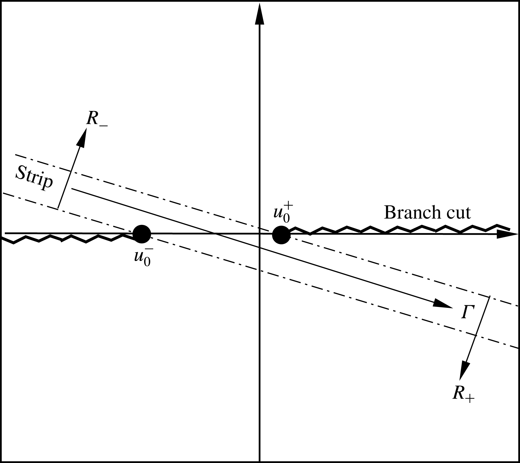
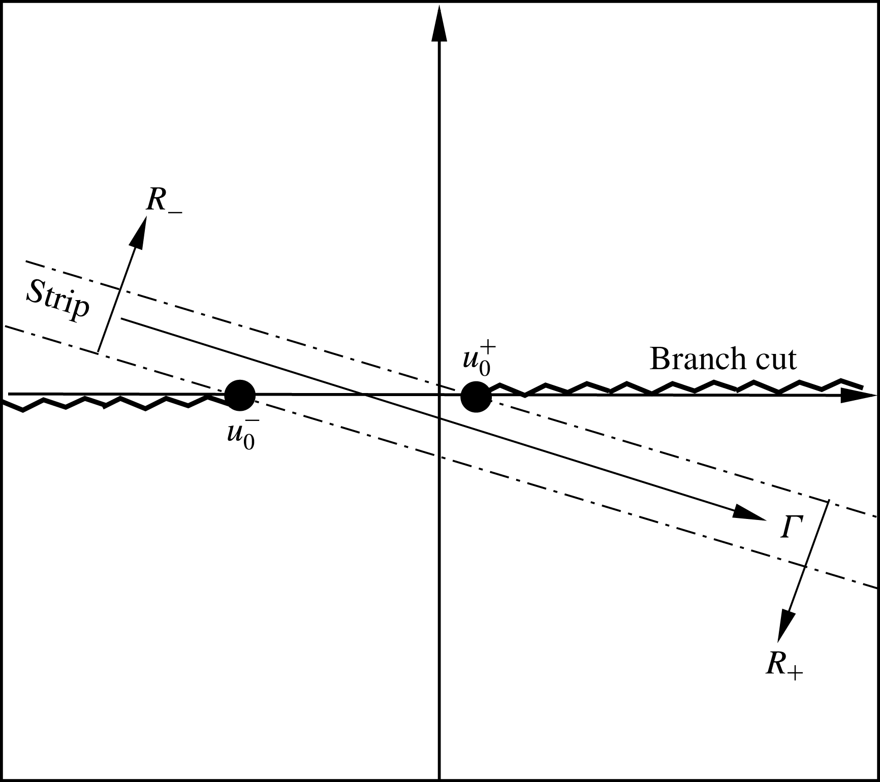
, which are regular on the two half-planes, respectively. For this problem, the two half-planes shown in figure 2 are defined as
 $$\begin{eqnarray}R_{\pm }:\quad \pm \!\text{Im}(u-u_{0}^{\pm })<\mp \!\tan ({\it\epsilon})\text{Re}(u-u_{0}^{\pm }),\end{eqnarray}$$
where
 $\tan ({\it\epsilon})=\text{Im}({\it\omega})/\text{Re}({\it\omega})$
. Here we use a complex frequency with a positive imaginary part to analyse unstable and causality conditions. The intersection of the two half-planes is a strip
 $\mathfrak{S}$
(see figure 2) of finite thickness, where all
 ${\it\beta}_{\pm }^{{\it\kappa}}$
and
 ${\it\beta}_{\pm }$
are regular.
Schematic of the two complex half-planes
 $R_{\pm }$
and the overlapped strip
 $\mathfrak{S}$
when
 $M=0.3$
. The path of integration
 ${\it\Gamma}$
will be slightly deformed around all possible acoustic zeros and poles and the hydrodynamic zeros.
Now we turn to the key part of the theoretical developments and provide the Wiener–Hopf equation related to our problem. First, we need to expand the vortex sheet displacements into Fourier series as follows:
 $$\begin{eqnarray}{\it\xi}(x,{\it\theta})=\mathop{\sum }_{{\it\kappa}=-\infty }^{+\infty }{\it\xi}^{{\it\kappa}}(x)\text{e}^{\text{i}{\it\kappa}{\it\theta}}.\end{eqnarray}$$
Then, by applying the conventional Fourier transform to (2.9) and adopting (2.16), we have
 $$\begin{eqnarray}A^{{\it\kappa}}(u)=-\frac{\text{i}(1-uM)}{{\it\lambda}\text{J}_{m+{\it\kappa}}^{\prime }({\it\lambda}{\it\omega})}F_{+}^{{\it\kappa}}(u),\end{eqnarray}$$
where
 $$\begin{eqnarray}F_{+}^{{\it\kappa}}(u)=\int _{0}^{+\infty }{\it\xi}^{{\it\kappa}}(x)\text{e}^{-\text{i}{\it\omega}ux}\,\text{d}x,\end{eqnarray}$$
and the relation
 ${\it\xi}(x,{\it\theta})=0$
when
 $x<0$
is implicitly adopted during the above derivation. In addition, here
 $(\cdot )_{+}$
denotes the regularity in the half-plane
 $R_{+}$
. Theoretically speaking, (2.19) suggests that the scattered field could be expressed by
 $F_{+}^{k}(u)$
, which can be further achieved by constructing the following important definition:
 $$\begin{eqnarray}\displaystyle G(u,{\it\theta}) & \hspace{-2.0pt}=\hspace{-2.0pt} & \displaystyle \underbrace{\int _{0}^{+\infty }-\text{i}{\it\omega}{\it\psi}(1^{+},{\it\theta},x)\text{e}^{-\text{i}{\it\omega}ux}\,\text{d}x}_{\text{I}}-\underbrace{\int _{0}^{+\infty }\left(-\text{i}{\it\omega}+M\frac{\partial }{\partial x}\right){\it\psi}_{s}(1^{-},{\it\theta},x)\text{e}^{-\text{i}{\it\omega}ux}\,\text{d}x}_{\text{II}}\nonumber\\ \displaystyle & \hspace{-2.0pt} & \displaystyle \hspace{-2.0pt}-\,\underbrace{\int _{-\infty }^{0}\left(-\text{i}{\it\omega}+M\frac{\partial }{\partial x}\right){\it\psi}_{s}(1^{-},{\it\theta},x)\text{e}^{-\text{i}{\it\omega}ux}\,\text{d}x}_{\text{III}}.\end{eqnarray}$$
This, in turn, can be simplified to the so-called Wiener–Hopf equation using the following steps. First, from (2.2a,b ) and (2.11), we have
 $$\begin{eqnarray}\text{term I}=\int _{0}^{+\infty }-p(x,1^{+},{\it\theta})\text{e}^{-\text{i}{\it\omega}ux}\,\text{d}x=\int _{0}^{+\infty }\text{i}{\it\omega}Z({\it\omega}){\it\xi}(x,{\it\theta})H({\it\theta})\text{e}^{-\text{i}{\it\omega}ux}\,\text{d}x,\end{eqnarray}$$
where
 $H({\it\theta})$
is periodic. To achieve the classical form of the Wiener–Hopf kernel (see (2.35) below), we represent the Fourier expansion of
 $H({\it\theta})$
as
 $H({\it\theta})=\sum _{{\it\kappa}=-\infty }^{+\infty }h^{{\it\kappa}}\exp (\text{i}{\it\kappa}{\it\theta})+1$
, with
 $$\begin{eqnarray}h^{{\it\kappa}}=\left\{\begin{array}{@{}ll@{}}\displaystyle \mathop{\sum }_{q=0}^{N-1}\text{e}^{-\text{i}{\it\kappa}q(2{\rm\pi}/N)}[{\it\gamma}(\text{e}^{-\text{i}{\it\kappa}l}-1)]/(-2\text{i}{\it\kappa}{\rm\pi}), & \text{if}~{\it\kappa}\neq 0,\\ {\it\gamma}Nl/2{\rm\pi}, & \text{if}~{\it\kappa}=0.\end{array}\right.\end{eqnarray}$$
From (2.23), we immediately find the following important relation:
 $$\begin{eqnarray}\mathop{\sum }_{q=0}^{N-1}\text{e}^{-\text{i}{\it\kappa}q(2{\rm\pi}/N)}=0,\end{eqnarray}$$
when
 ${\it\kappa}\neq 0,\pm N,\pm 2N,\ldots$
. The algebraic developments related to (2.23) and (2.24) are straightforward and are therefore omitted for brevity. It is worthwhile to emphasise that
 $h^{{\it\kappa}}$
would exclusively describe the acoustic effects owing to the rigid splices. Substituting (2.23) into (2.22), we have
 $$\begin{eqnarray}\text{term I}=\text{i}{\it\omega}Z({\it\omega})\mathop{\sum }_{{\it\kappa}_{1}=-\infty }^{+\infty }\mathop{\sum }_{{\it\kappa}_{2}=-\infty }^{+\infty }h^{{\it\kappa}_{1}}F_{+}^{{\it\kappa}_{2}}\text{e}^{\text{i}{\it\theta}({\it\kappa}_{1}+{\it\kappa}_{2})}+\text{i}{\it\omega}Z({\it\omega})\mathop{\sum }_{{\it\kappa}=-\infty }^{+\infty }F_{+}^{{\it\kappa}}\text{e}^{\text{i}{\it\kappa}{\it\theta}}.\end{eqnarray}$$
Next, according to (2.16), we have
 $$\begin{eqnarray}\text{terms II}+\text{III}=\mathop{\sum }_{{\it\kappa}=-\infty }^{+\infty }\frac{{\it\omega}(1-uM)^{2}}{{\it\lambda}}\frac{\text{J}_{m+{\it\kappa}}({\it\lambda}{\it\omega})}{\text{J}_{m+{\it\kappa}}^{\prime }({\it\lambda}{\it\omega})}F_{+}^{{\it\kappa}}\text{e}^{\text{i}{\it\kappa}{\it\theta}}.\end{eqnarray}$$
We further define
 $G_{+}(u)$
as follows, and will be able to find its analytical expression,
 $$\begin{eqnarray}G_{+}(u)~\stackrel{{\rm\Delta}}{=}\text{terms I}+\text{II}=\frac{1-{\it\mu}_{mn}^{+}M}{{\it\mu}_{mn}^{+}-u}\text{J}_{m}({\it\alpha}_{mn}),\end{eqnarray}$$
which is obtained by using the pressure continuity condition (2.8), and the definition of the incident wave (2.4). Meanwhile, we define
 $G_{-}(u,{\it\theta})\stackrel{{\rm\Delta}}{=}\text{term III}$
, which is unknown but still can be expanded into a Fourier series as
 $G_{-}(u,{\it\theta})=\sum _{{\it\kappa}=-\infty }^{+\infty }G_{-}^{{\it\kappa}}(u)\text{e}^{\text{i}{\it\kappa}{\it\theta}}$
.
Finally, we obtain the Wiener–Hopf kernel equation:
 $$\begin{eqnarray}\displaystyle G_{-}(u,{\it\theta})+G_{+}(u) & \hspace{-2.0pt}=\hspace{-2.0pt} & \displaystyle \text{i}{\it\omega}Z({\it\omega})\mathop{\sum }_{{\it\kappa}_{1}=-\infty }^{+\infty }\mathop{\sum }_{{\it\kappa}_{2}=-\infty }^{+\infty }h^{{\it\kappa}_{1}}F_{+}^{{\it\kappa}_{2}}\text{e}^{\text{i}{\it\theta}({\it\kappa}_{1}+{\it\kappa}_{2})}\nonumber\\ \displaystyle & \hspace{-2.0pt} & \displaystyle \hspace{-2.0pt}+\,\mathop{\sum }_{{\it\kappa}=-\infty }^{+\infty }\left[\frac{{\it\omega}(1-uM)^{2}}{{\it\lambda}}\frac{\text{J}_{m+{\it\kappa}}({\it\lambda}{\it\omega})}{\text{J}_{m+{\it\kappa}}^{\prime }({\it\lambda}{\it\omega})}+\text{i}{\it\omega}Z({\it\omega})\right]F_{+}^{{\it\kappa}}\text{e}^{\text{i}{\it\kappa}{\it\theta}}.\end{eqnarray}$$
This leads to a system of linear equations by equating terms with the same
 $\exp (\text{i}{\it\kappa}{\it\theta})$
:
 $$\begin{eqnarray}\boldsymbol{G}_{-}(u)+\boldsymbol{G}_{+}(u)=(\unicode[STIX]{x1D63E}+\unicode[STIX]{x1D646}(u))\boldsymbol{F}_{+}(u)=\hat{\unicode[STIX]{x1D646}}\boldsymbol{F}_{+}(u),\end{eqnarray}$$
with
 $$\begin{eqnarray}\displaystyle & \displaystyle \boldsymbol{G}_{-}=[\ldots ,G_{-}^{-{\it\kappa}},\ldots ,G_{-}^{0},\ldots ,G_{-}^{{\it\kappa}}], & \displaystyle\end{eqnarray}$$
 $$\begin{eqnarray}\displaystyle & \displaystyle \boldsymbol{G}_{+}=[\ldots ,0,\ldots ,0,G_{+},0,\ldots ,0,\ldots ], & \displaystyle\end{eqnarray}$$
 $$\begin{eqnarray}\displaystyle & \displaystyle \unicode[STIX]{x1D63E}=(\unicode[STIX]{x1D60A})_{ij}=(\text{i}{\it\omega}Z({\it\omega})h^{i-j}), & \displaystyle\end{eqnarray}$$
 $$\begin{eqnarray}\displaystyle & \displaystyle \unicode[STIX]{x1D646}=\text{diag}(\unicode[STIX]{x1D612}^{{\it\kappa}}), & \displaystyle\end{eqnarray}$$
 $$\begin{eqnarray}\displaystyle & \displaystyle \boldsymbol{F}_{+}=[\ldots ,F_{+}^{-{\it\kappa}},\ldots ,F_{+}^{0},\ldots ,F_{+}^{{\it\kappa}},\ldots ], & \displaystyle\end{eqnarray}$$
 $(\unicode[STIX]{x1D60A})_{ij}$
is the entry in the
 $i$
th row and
 $j$
th column of the constant matrix
 $\unicode[STIX]{x1D63E}$
, which is solely determined by the circumferential layout of liner splices, and
 $\text{diag}(\unicode[STIX]{x1D612}^{{\it\kappa}})$
represents a diagonal matrix with
 $\unicode[STIX]{x1D612}^{{\it\kappa}}$
(
 ${\it\kappa}$
from
 $-\infty$
to
 $\infty$
) as the main diagonal entries, where
 $$\begin{eqnarray}\unicode[STIX]{x1D612}^{{\it\kappa}}(u)=\frac{{\it\omega}(1-uM)^{2}}{{\it\lambda}}\frac{\text{J}_{m+{\it\kappa}}({\it\lambda}{\it\omega})}{\text{J}_{m+{\it\kappa}}^{\prime }({\it\lambda}{\it\omega})}+\text{i}{\it\omega}Z({\it\omega}).\end{eqnarray}$$
2.3. Kernel properties
In the classical Wiener–Hopf method,
 $\hat{\unicode[STIX]{x1D646}}$
is the so-called Wiener–Hopf kernel, which characterises the dispersion relations of the problem. However, our problem with liner splices has a matrix kernel. Previous endeavours in matrix factorisations have mostly been developed for matrix kernels of small size 2 (Veitch & Peake Reference Veitch and Peake2008). An effective factorisation method for matrix kernels of a large size is still not available. However, it is easy to see that our matrix kernel
 $\hat{\unicode[STIX]{x1D646}}$
is quite special, involving a constant matrix
 $\unicode[STIX]{x1D63E}$
and a diagonal matrix
 $\unicode[STIX]{x1D646}$
. The latter can be split using existing scalar factorisation techniques (Gabard & Astley Reference Gabard and Astley2006).
Before the development of analytical solutions for our problem, it is necessary to discuss the properties of the diagonal matrix
 $\unicode[STIX]{x1D646}$
. The poles and zeros of
 $\unicode[STIX]{x1D646}$
can be examined by solving
 $\text{det}(\unicode[STIX]{x1D646}(u))=\prod _{k}\!\unicode[STIX]{x1D612}^{{\it\kappa}}$
. Given
 ${\it\kappa}$
, the properties of the corresponding
 $\unicode[STIX]{x1D612}^{{\it\kappa}}(u)$
in (2.35) should be exactly the same as scalar kernels appearing in previous works (Rienstra Reference Rienstra2003a
, Reference Rienstra2007), where the kernel properties have been carefully examined using both low-frequency and high-frequency asymptotic methods. In particular, the asymptotic expression at high frequency,
 $\text{J}_{m}(x)\approx \text{exp}(\text{i}x-\text{i}m{\rm\pi}/2-\text{i}{\rm\pi}/4)/\sqrt{2{\rm\pi}x}$
when
 $(x\rightarrow \infty ,~\text{Im}(x)<0)$
, is only valid if
 $m<O(x)$
. However, from the above Fourier series expansions, we already know that the splices would excite scattering waves of various circumferential modes,
 $m+{\it\kappa}$
, where
 ${\it\kappa}$
could be any integer. To use this asymptotic expression given by Rienstra (Reference Rienstra2003a
, Reference Rienstra2007), we have to suppose
 $|m+{\it\kappa}|<{\it\lambda}{\it\omega}$
for any given
 ${\it\kappa}$
as
 ${\it\omega}\rightarrow \infty$
.
The remaining manipulations, such as branch cuts and removal of unstable zeros, are almost the same as in the previous works (Rienstra Reference Rienstra2003a
, Reference Rienstra2007). Figure 2 shows the two branch cuts, the two half-planes
 $R_{\pm }$
and the integral path
 ${\it\Gamma}$
. It can be seen that one branch cut is slightly above the abscissa axis and the other is slightly below the abscissa axis. The integral path is slightly deformed to be a parabola (Gabard & Astley Reference Gabard and Astley2006, appendix A) when
 ${\it\epsilon}\rightarrow 0$
around any possible acoustic zeros and poles and the hydrodynamic zeros. From (2.35) it is easy to see that
 $\unicode[STIX]{x1D612}^{{\it\kappa}}\sim O(u^{1})$
as
 $|u|\rightarrow \infty$
in the overlapped strip
 $\mathfrak{S}$
.
2.4. Solutions
For each scalar
 $\unicode[STIX]{x1D612}^{{\it\kappa}}$
, we are able to obtain the corresponding factorisation by using the readily available Cauchy-type integral formulations (Gabard & Astley Reference Gabard and Astley2006):
 $$\begin{eqnarray}\unicode[STIX]{x1D612}^{{\it\kappa}}=\frac{\unicode[STIX]{x1D612}_{+}^{{\it\kappa}}}{\unicode[STIX]{x1D612}_{-}^{{\it\kappa}}},\end{eqnarray}$$
where
 $\unicode[STIX]{x1D612}_{\pm }^{{\it\kappa}}$
and the corresponding reciprocals are regular and non-zero in
 $R_{\pm }$
, respectively. Taking this all together, we have
 $$\begin{eqnarray}\unicode[STIX]{x1D646}_{\pm }=\text{diag}(\unicode[STIX]{x1D612}_{\pm }^{{\it\kappa}}),\quad \unicode[STIX]{x1D646}_{\pm }^{-1}=\text{diag}(1/\unicode[STIX]{x1D612}_{\pm }^{{\it\kappa}}).\end{eqnarray}$$
Then, (2.29) is reformulated to
 $$\begin{eqnarray}[\unicode[STIX]{x1D63E}+\unicode[STIX]{x1D646}_{-}^{-1}(u)\unicode[STIX]{x1D646}_{+}(u)]\boldsymbol{F}_{+}(u)=\boldsymbol{G}_{-}(u)+\boldsymbol{G}_{+}(u),\end{eqnarray}$$
which leads to
 $$\begin{eqnarray}[\unicode[STIX]{x1D646}_{-}(u)\unicode[STIX]{x1D63E}+\unicode[STIX]{x1D646}_{+}(u)]\boldsymbol{F}_{+}(u)=\unicode[STIX]{x1D646}_{-}(u)\boldsymbol{G}_{-}(u)+\unicode[STIX]{x1D646}_{-}(u)\boldsymbol{G}_{+}(u)\end{eqnarray}$$
by rearranging terms according to their regularity properties. More specifically, the left-hand and right-hand sides should be regular in the two complex
 $u$
planes, i.e.
 $R_{+}$
and
 $R_{-}$
, respectively. By definition, we know that
 $\unicode[STIX]{x1D646}_{\pm }(u)$
is regular and non-zero in
 $R_{\pm }$
, respectively; and that
 $\boldsymbol{F}(u)$
is regular in
 $R_{+}$
and
 $\boldsymbol{G}_{-}(u)$
is regular in
 $R_{-}$
. On the other hand, (2.27) suggests that
 $\boldsymbol{G}_{+}(u)$
is regular in the whole
 $u$
plane except for the single pole
 ${\it\mu}_{mn}^{+}$
, which can be cancelled out by introducing an additional term,
 $-\unicode[STIX]{x1D646}_{-}({\it\mu}_{mn}^{+})\boldsymbol{G}_{+}(u)$
, on both sides of (2.39). The first term on the left-hand side, however, is still not regular in
 $R_{+}$
. To resolve this issue, we simply adopt the following approximation:
 $$\begin{eqnarray}\unicode[STIX]{x1D646}_{-}(u)\sim \unicode[STIX]{x1D646}_{-}({\it\mu}_{mn}^{+}),\end{eqnarray}$$
where the right-hand side is regular on the whole
 $u$
plane, and can be regarded as the simplest Taylor expansion of
 $\unicode[STIX]{x1D646}_{-}(u)$
. The appropriateness of this approximation for various case set-ups will be tested in the next section. We should say that this undesirable approximation could compromise the modelling method for more generic cases, such as azimuthally non-uniform liner studies, although all the rest of the proposed modelling method is rigorous. However, we have to adopt this approximation in the current work, since a generic factorisation method for a matrix kernel with size larger than
 $2\times 2$
is still not available.
Substituting (2.40) into (2.39), we can obtain
 $$\begin{eqnarray}\displaystyle & & \displaystyle [\unicode[STIX]{x1D646}_{-}({\it\mu}_{mn}^{+})\unicode[STIX]{x1D63E}+\unicode[STIX]{x1D646}_{+}(u)]\boldsymbol{F}_{+}(u)-\unicode[STIX]{x1D646}_{-}({\it\mu}_{mn}^{+})\boldsymbol{G}_{+}(u)\nonumber\\ \displaystyle & & \displaystyle \quad =\unicode[STIX]{x1D646}_{-}(u)\boldsymbol{G}_{-}(u)+[\unicode[STIX]{x1D646}_{-}(u)-\unicode[STIX]{x1D646}_{-}({\it\mu}_{mn}^{+})]\boldsymbol{G}_{+}(u).\end{eqnarray}$$
To this end, the left- and right-hand sides of (2.41) should be regular on
 $R_{+}$
and
 $R_{-}$
, respectively. As a result, (2.41) is satisfied in the intersection strip of
 $R_{\pm }$
. By analytical continuation, (2.41) defines an entire function
 $\boldsymbol{E}(u)$
that is regular on the whole complex
 $u$
plane.
According to Noble (Reference Noble1958) and
 $\unicode[STIX]{x1D612}^{{\it\kappa}}\sim O(u^{1})$
, we have
 $\unicode[STIX]{x1D612}_{\pm }^{{\it\kappa}}(u,{\it\theta})\sim O(u^{\pm 1/2})$
. If
 $M>0$
, we apply a full Kutta condition (Gabard & Astley Reference Gabard and Astley2006) at
 $(x,r)=(0,1)$
, resulting in
 ${\it\psi}(x,1)=O(x^{3/2})$
as
 $x\rightarrow 0$
, which transforms into
 $F_{+}^{{\it\kappa}}(u)=O(u^{-5/2})$
as
 $|u|\rightarrow \infty$
. For inlet cases with
 $M<0$
, we use the leading-edge condition such that
 ${\it\psi}(x,1)=O(x^{1/2})$
as
 $x\rightarrow 0$
, which leads to
 $F_{+}^{{\it\kappa}}(u)=O(u^{-3/2})$
as
 $|u|\rightarrow \infty$
(Gabard & Astley Reference Gabard and Astley2006). For both cases, from (2.41) we have
 $\boldsymbol{G}_{-}(u)\leqslant O(u^{-1/2})$
and
 $\boldsymbol{E}(u)=0$
as
 $|u|\rightarrow \infty$
.
To this end, we have
 $$\begin{eqnarray}[\unicode[STIX]{x1D646}_{-}({\it\mu}_{mn}^{+})\unicode[STIX]{x1D63E}+\unicode[STIX]{x1D646}_{+}(u)]\boldsymbol{F}_{+}(u)=\unicode[STIX]{x1D646}_{-}({\it\mu}_{mn}^{+})\boldsymbol{G}_{+}(u).\end{eqnarray}$$
Solving the equation set we can obtain
 $F_{+}^{{\it\kappa}}(u)$
.
The scattered field can be solved by using the inverse Fourier transform for each scattering mode, i.e.
 $$\begin{eqnarray}{\it\psi}_{s}^{{\it\kappa}}(x,r)=\frac{{\it\omega}}{2{\rm\pi}\text{i}}\int _{{\it\Gamma}}\frac{(1-uM)F_{+}^{{\it\kappa}}(u)}{{\it\lambda}}\frac{\text{J}_{m+{\it\kappa}}({\it\lambda}{\it\omega}r)}{\text{J}_{m+{\it\kappa}}^{\prime }({\it\lambda}{\it\omega})}\text{e}^{\text{i}{\it\omega}ux}\,\text{d}u,\end{eqnarray}$$
where
 ${\it\Gamma}$
is an integral path defined in the strip
 $\mathfrak{S}$
. Eventually, we obtain the whole scattered field by linear superposition as follows:
 $$\begin{eqnarray}{\it\psi}_{s}(x,r,{\it\theta})=\mathop{\sum }_{{\it\kappa}=-\infty }^{\infty }{\it\psi}_{s}^{{\it\kappa}}(r,x)\text{e}^{\text{i}{\it\kappa}{\it\theta}}.\end{eqnarray}$$
Given
 ${\it\psi}_{s}(x,r,{\it\theta})$
, the corresponding acoustic potential
 ${\it\phi}_{s}$
and sound pressure
 $p$
can be easily obtained by using (2.6) and (2.2a,b
), respectively.
3. Results and discussion
3.1. Validation
First, the infinite sum of Fourier series for
 $H({\it\theta})$
has to be truncated at a finite number
 $T_{N}$
in the numerical implementation. As a result, the infinite matrix
 $\hat{\unicode[STIX]{x1D646}}$
is accordingly truncated to
 $(2T_{N}+1)\times (2T_{N}+1)$
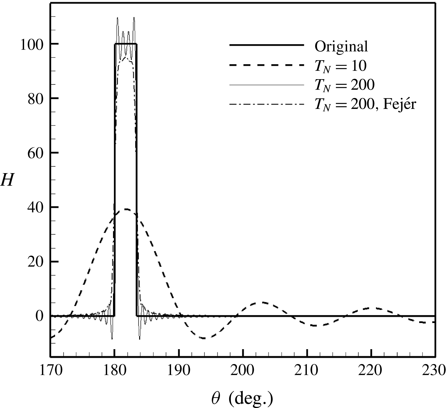
dimensions. To examine the truncation effect, the reconstructed
 $H({\it\theta})$
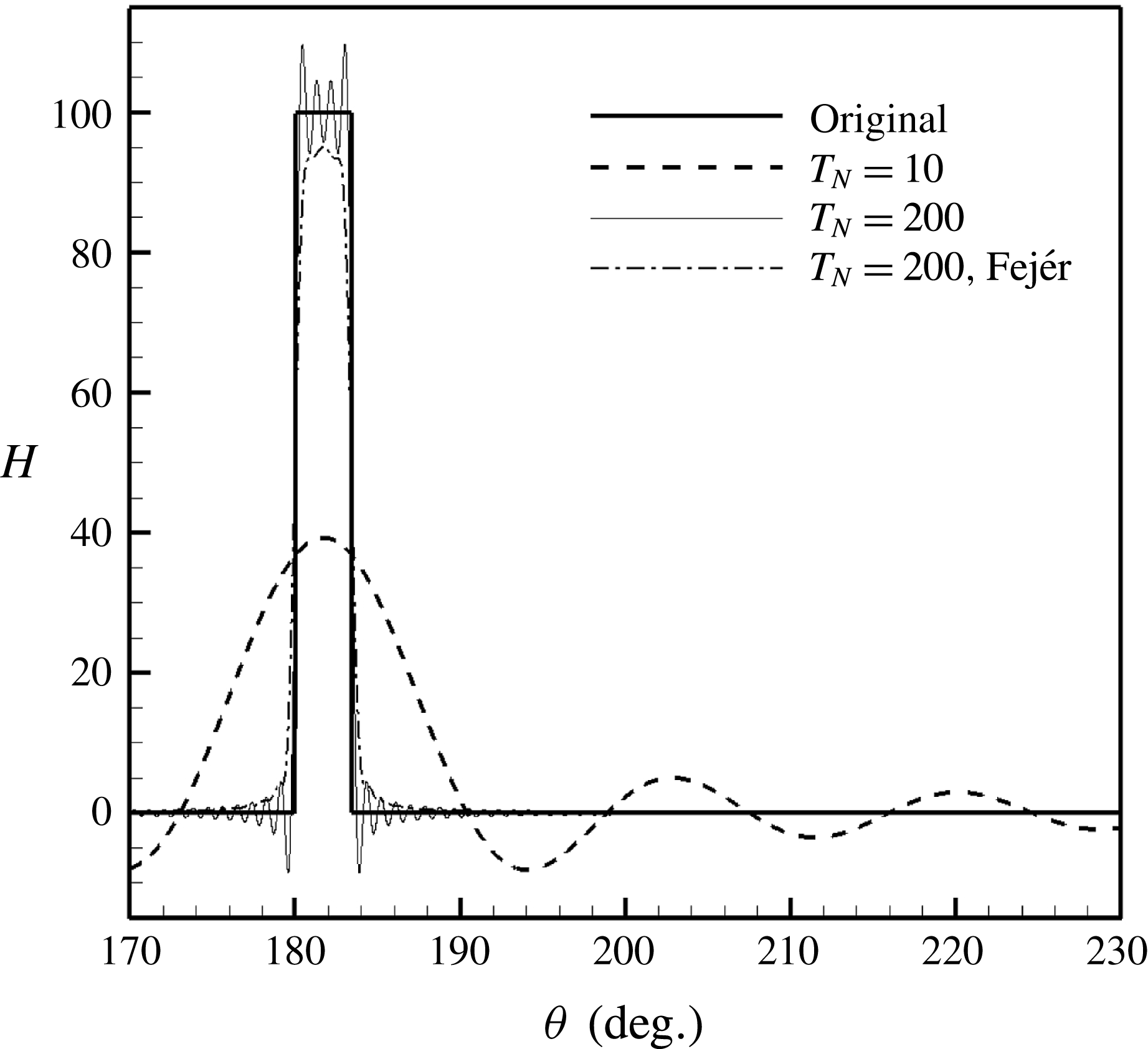
is shown in figure 3, which shows that a larger number
 $T_{N}$
, such as 200, would yield a better reconstruction of
 $H({\it\theta})$
. Therefore, the truncation number
 $T_{N}$
is set to 200 in the following numerical calculations. In addition to the classical Fourier series reconstruction, we have tested Fejér summation to suppress the Gibbs phenomenon appearing at the jump discontinuity. Figure 3 shows that the corresponding reconstruction is smoothed by this treatment. However, the follow-up numerical validations suggest that this smooth Fejér summation would lead to undesirable solutions. As a result, the rest of this work adopts the classical Fourier series summation.
Reconstructed
 $H({\it\theta})$
with different truncation numbers
 $T_{N}$
(from 10 to 250; for clarity only two results are shown here). The original
 $H({\it\theta})$
is also shown here (the solid line) as a comparison. The splice number is
 $N=2$
and the splice width
 $l=0.06$
. For clarity, only a part of
 $H({\it\theta})$
is shown. Here the region with the rigid splice is between
 ${\it\theta}=180$
° and 183.44°.
We implement the whole theoretical model with MATLAB
 $^{\unicode[STIX]{x00AE} }$
to obtain numerical solutions on three-dimensional grids that consist of
 $256\times 64\times 721$
grid points for the geometrical domain of
 $-2\leqslant x\leqslant 2$
,
 $0\leqslant r\leqslant 1$
and
 $0\leqslant {\it\theta}\leqslant 2{\rm\pi}$
. The computational cost on a desktop with Intel
 $^{\unicode[STIX]{x00AE} }$
Core i5 processor at 3.30 GHz is about 700 s with 3.2 GB memory. As a comparison, a similar case set-up was solved by the typical commercial finite element software ACTRAN
 $^{\unicode[STIX]{x00AE} }$
using unstructured meshes with
 $3\times 10^{6}$
grid points on a computational server with Intel Core E5 processor at 2.50 GHz. The computational cost is almost 58 000 s with 46 GB memory. It can be seen that the theoretical model is much more computationally efficient by almost two orders of magnitude.
Comparison of instantaneous sound pressure at
 $(x,r)=(0.3,1)$
with respect to
 ${\it\theta}$
, where
 $(m,n)=(24,1)$
,
 $Z({\it\omega})=2+\text{i}$
at
 ${\it\omega}=30$
,
 $l=0.06$
,
 $N=2$
and (a)
 $M=0$
and (b)
 $M=0.3$
. The amplitude of the incident wave is set to 0.2. The solutions are obtained by the theoretical Wiener–Hopf solver (denoted ‘WH’) and the ACTRAN solver (denoted ‘Numerical’), respectively. The arrows denote the regions with rigid splices.

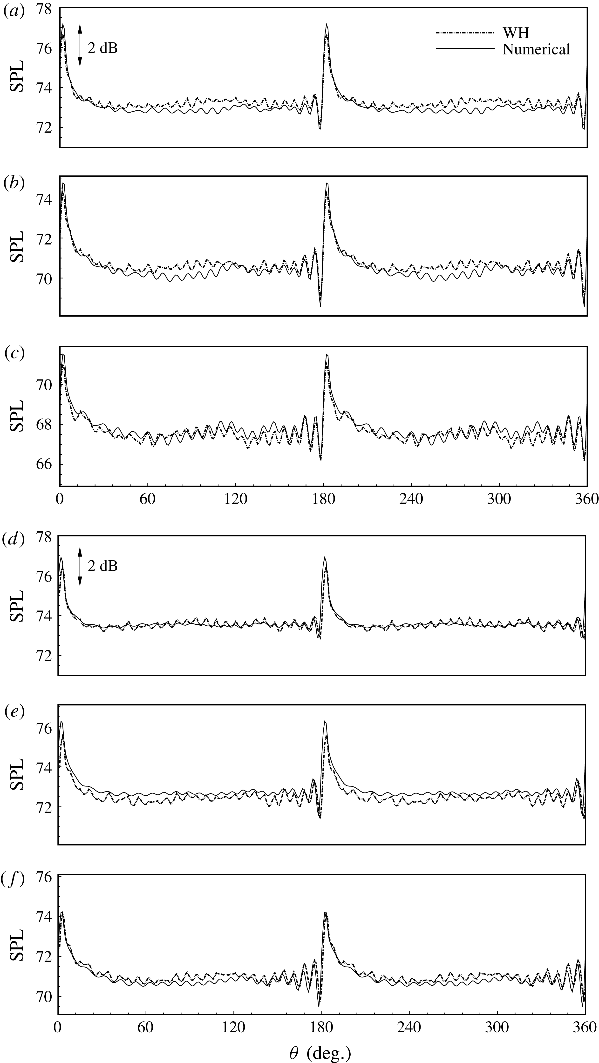
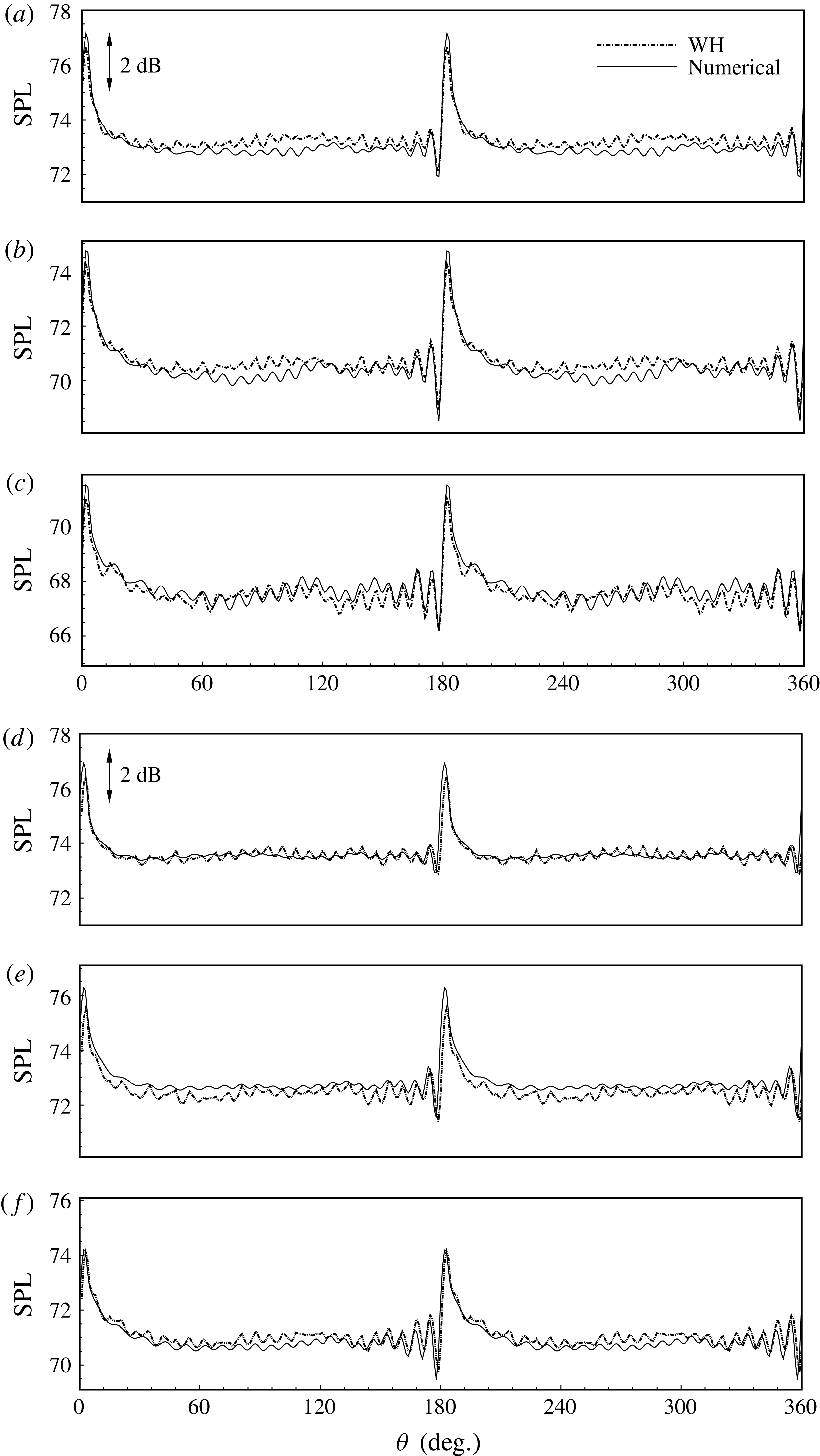
The SPL results at
 $(x,r)=(0.1,1)$
(a,d),
 $(0.2,1)$
(b,e) and
 $(0.3,1)$
(c,f). Other set-ups are the same as those in figure 4.
To validate the theoretical model, we compare sound pressure profiles at
 $(x,r)=(0.3,1)$
, which is the wall surface close to the axial hard–soft interface, with and without a background flow. Figure 4 shows the instantaneous solutions (with respect to
 ${\it\theta}$
) from the theoretical model and the numerical commercial solver. It can be seen that the two solutions are almost identical, which helps to validate the current theoretical model. To further quantify the difference, figure 5 shows some more results of the corresponding sound pressure level (SPL), which is defined as
 $$\begin{eqnarray}\text{SPL}=20\log _{10}\frac{p_{rms}}{2\times 10^{-5}},\end{eqnarray}$$
where
 $p_{rms}$
is the root mean square of sound pressure at
 $(x,r)=(0.1,1),~(0.2,1)$
and
 $(0.3,1)$
. It can be seen that the analytical results and the numerical results agree very well in most regions, with the largest difference less than 0.7 dB. In particular, the wiggles of the SPL results around the splices are well captured by the theoretical model. We believe that this discrepancy between the numerical solver and the theoretical model may possibly come from the approximation, (2.40), adopted in the above theoretical developments.
Figures 4 and 5 also show that sound waves are less attenuated in the regions with rigid splices than in the lined regions, which would therefore excite new circumferential modes other than the modes of incident waves, and the new modes should be related to the layout of splices in some way. More detailed analysis and discussion will be given in § 3.3. It is worthwhile to mention that the non-dimensional parameters are deliberately chosen in this work to represent typical design and working conditions of aeroengines.
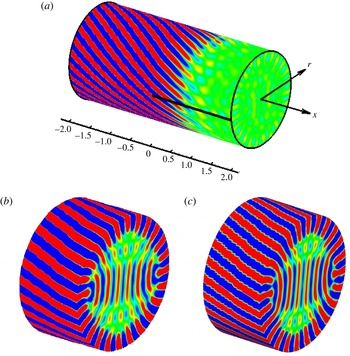
(a) An instantaneous sound pressure field, with incident spinning modes
 $(m,n)=(24,1)$
, Mach number
 $M=0.3$
, impedance of lined surface
 $Z({\it\omega})=2+\text{i}$
at
 ${\it\omega}=30$
, splice width
 $l=0.06$
and splice number
 $N=2$
. The amplitude of the incident wave is set to 0.2. Here only one splice is visible, which is represented by a thick, straight line. The sound pressure field is shown between
 $\pm 0.02$
using 21 levels to make visible the largely attenuated waves in the lined region at
 $x\geqslant 0$
. In contrast, the wave patterns of the upstream-directed scattering waves due to splices are only slightly visible between
 $-2<x<0$
. (b,c) Instantaneous sound pressure fields for
 $x\in [-0.5,0.5]$
are shown between
 $\pm 0.08$
using 21 levels. It can be seen that the results from the WH analytical model (b) and the numerical solver (c) have almost identical patterns.

3.2. Scattered fields
Sound propagating in a lined duct with splices contains both incident and scattered sound waves. The latter component is excited by various hard–soft interfaces in the axial and circumferential directions and will propagate inside the duct in both upstream and downstream directions. Both the incident and scattered waves will be attenuated during the propagation along the lining surfaces. As an example, figure 6 shows the analytical solution of one instantaneous sound pressure field. Here the cylinder accommodates an incident wave of a single spinning mode,
 $(m,n)=(24,1)$
, with a uniform subsonic flow. Figure 6 shows that the lining surface gradually attenuates the propagating acoustic power. However, the hard–soft interface at
 $x=0$
between the left rigid wall and the right lined wall would excite new spinning modes in the radial direction, whilst the hard–soft interfaces in the
 ${\it\theta}$
direction between the rigid splices and the lining surface would excite new spinning modes mainly in the circumferential direction. In addition, figure 6(a) shows that the incident wave is greatly attenuated beyond
 $x=0.5$
. Hence, the computational domain is set to
 $x\in [-0.6,0.6]$
to save computational costs. Figure 6(b) compares the prediction results from the analytical model and the numerical solver. Here we deliberately show the two results between
 $\pm 0.08$
using 21 levels to highlight any possible difference. Nevertheless, figure 6(b) suggests that the two results are almost identical.
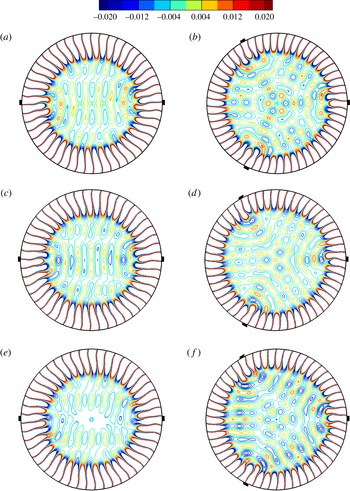
Instantaneous sound pressure fields in the
 $(r,{\it\theta})$
cross-section at
 $x=0.1$
. (a,c,e) The set-up is
 $(m,n)=(24,1)$
,
 ${\it\omega}=30$
(corresponding time period is 0.21) and Mach number
 $M=0.5$
; and number of splices is
 $N=2$
, starting from
 ${\it\theta}=0$
and
 ${\rm\pi}$
: (a)
 $t=0.01$
, (b)
 $t=0.03$
and (c)
 $t=0.9$
. (b,d,f) The set-up is
 $(m,n)=(27,1)$
,
 ${\it\omega}=32$
(corresponding time period is 0.19) and Mach number
 $M=0.3$
; and number of splices is
 $N=3$
, starting from
 ${\it\theta}=0$
,
 $2{\rm\pi}/3$
and
 $4{\rm\pi}/3$
: (d)
 $t=0.10$
, (e)
 $t=0.14$
and (f)
 $t=0.15$
. Other parameters are impedance
 $Z=2+\text{i}$
and splice width
 $l=0.06$
. The contours are all shown between
 $\pm 0.02$
using 11 levels. The splices are illustrated by dark rectangles in each panel.

Figure 7 shows analytical solutions of some instantaneous sound pressure fields (with representative time within one period) of the
 $(r,{\it\theta})$
cross-section at
 $x=0.1$
. Here we show two different representative set-ups with
 $N=2$
and 3, respectively. It can be seen that the incident waves are still dominant in this cross-section. However, scattering waves from axial and circumferential hard–soft interfaces are slightly visible, which eventually result in various patterns across the whole cross-section. In particular, figure 7(a–c) shows new patterns with various circumferential and radial modes. On the other hand, figure 7(d–f) shows more distinctive patterns inside the duct, which clearly suggests the appearance of scattering waves with large radial mode numbers, persistently evolving in the angular sectors corresponding to the three axial splices.
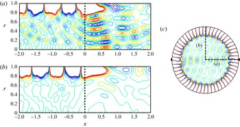
An instantaneous sound pressure field of
 $(x,r)$
cross-section, with
 $(m,n)=(27,1)$
,
 ${\it\omega}=32$
,
 $M=0.3$
,
 $Z=2+\text{i}$
,
 $l=0.06$
and
 $N=2$
. The amplitude of the incident wave is set to 0.2. The contour is shown here between
 $\pm 0.02$
using 21 levels. The circumferential positions of (a) and (b) can be found in (c), where the splices are illustrated by dark rectangles.

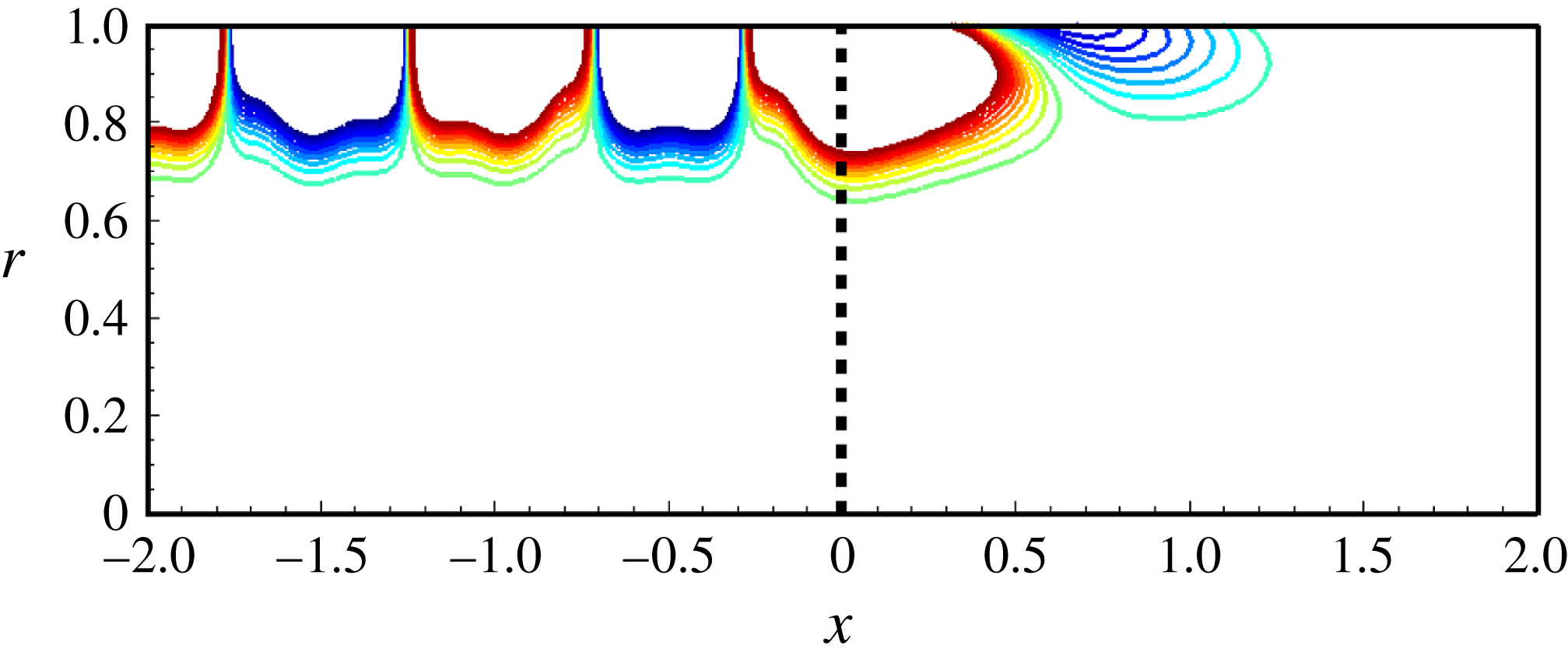
The model set-up and display style are the same as figure 8 except for the splice width
 $l=0$
, i.e. without splices.
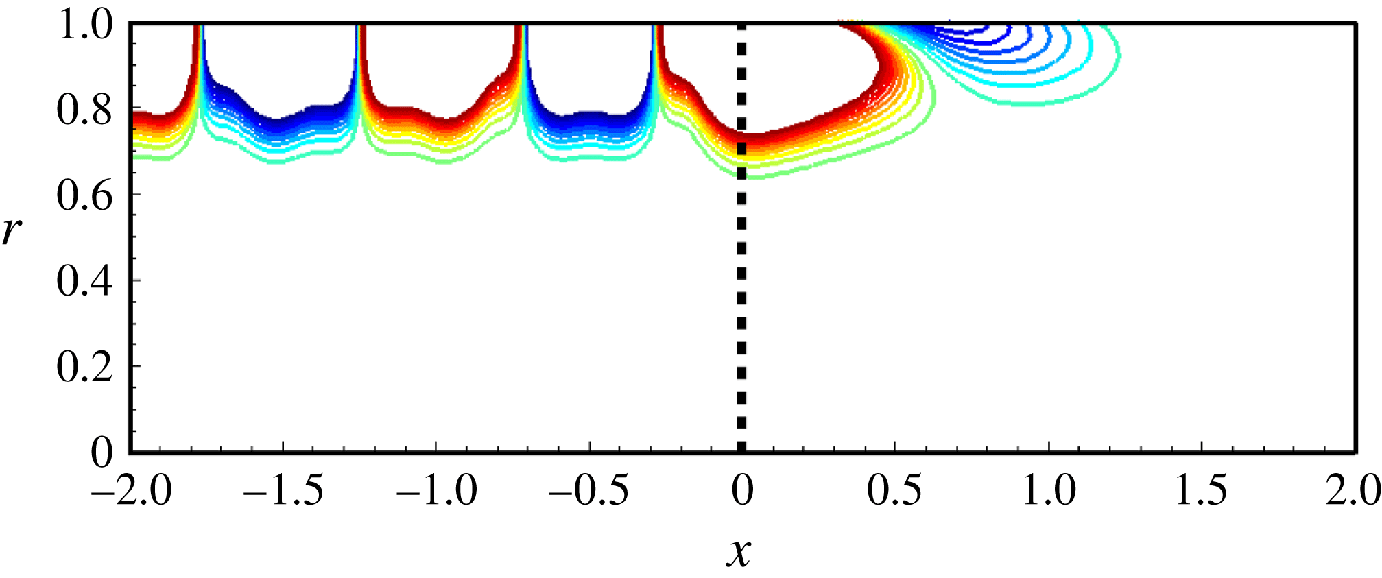
Figure 7 clearly shows the apparent connections between these scattering wave patterns inside the duct and the number of splices. To further examine this finding, figure 8 shows the instantaneous sound pressure field of two different
 $(x,r)$
cross-sections. The number of splices is
 $N=2$
. The vertical dashed lines denote the position of the axially hard–soft interface at
 $x=0$
. As marked in figure 8(c), cross-section (a) is aligned with the centre of the rigid splice, and cross-section (b) is placed most away from the two rigid splices. Figure 8(a,b) clearly shows that scattered patterns mainly develop in the region with rigid splices. As a comparison, figure 9 shows the sound pressure field of a typical duct case with a semi-infinite lined region at
 $x>0$
(Rienstra Reference Rienstra2003a
). Here the splices are absent and the other parameters are still the same as those in figure 8. Contrary to the liner splice cases in figure 8, the instantaneous sound pressure field for the uniformly lined duct is axisymmetric and free from redundant circumferential and radial modes. Therefore, the effect of liner splices on scattered acoustic fields is clearly demonstrated here. We should mention that the analytical solution shown in figure 9 is produced by our current theoretical model by simply setting the width of splices
 $l$
to zero. The corresponding results are validated by our in-house numerical solver (Huang, Zhong & Liu Reference Huang, Zhong and Liu2014; Liu, Huang & Zhang Reference Liu, Huang and Zhang2014) and ACTRAN, respectively.
Modal spectrum of instantaneous sound pressure level at
 $x=0.1$
shown with respect to circumferential and radial modes. The parameter set-ups are: (a)
 $(m,n)=(24,1)$
,
 $M=0.5$
,
 $Z=2+\text{i}$
at
 ${\it\omega}=30$
,
 $l=0.06$
,
 $N=2$
; and (b)
 $(m,n)=(27,1)$
,
 $M=0.3$
,
 $Z=2+\text{i}$
at
 ${\it\omega}=32$
,
 $l=0.06$
,
 $N=3$
.

3.3. Scattering modes and analysis
Further analysis is performed here to deepen the understanding of the effect of liner splices. First, by carefully examining (2.23), (2.24) and (2.28), we would have
 $F_{+}^{{\it\kappa}}=0$
, and consequently
 ${\it\psi}_{s}^{{\it\kappa}}=0$
when
 ${\it\kappa}\neq 0,\pm N,\pm 2N,\ldots$
. In other words, if the circumferential mode of an incident sound wave is
 $m$
, the corresponding circumferential modes of scattered fields in a lined duct with
 $N$
splices are always
 $m$
,
 $m\pm N$
,
 $m\pm 2N,\ldots$
. Therefore, (2.24) theoretically explains the famous Tyler–Sofrin rule (Tyler & Sofrin Reference Tyler and Sofrin1962) that describes the mode selection appearing in scattering waves due to rigid splices.
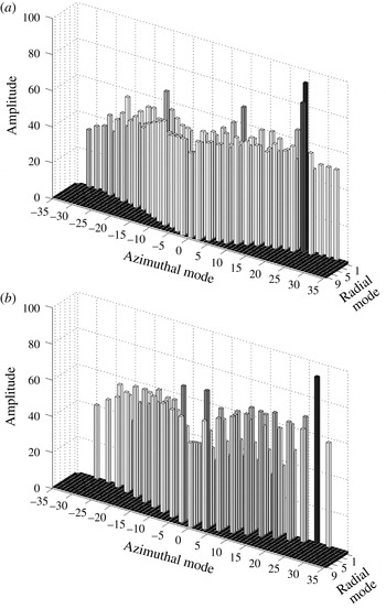
To clearly demonstrate this scattering mode selection, figure 10 shows the amplitude of the modal spectrum for the whole SPL fields at
 $x=0.1$
. The case set-ups are the same as the two previous ones in figure 7. It can be seen that various new radial and circumferential modes are excited. Theoretically speaking, scattering waves with a low circumferential mode number are inclined to cut-on and would therefore compromise noise control performance. On the other hand, scattering waves with high circumferential and radial modes are prone to cut-off. Equation (2.24) already predicts that the circumferential modes should be selected by the
 $N$
splices, and here
 $N=2$
and 3. Exactly as the predictions, the non-zero value appears in every two circumferential modes in figure 10(a), while the non-zero value appears in every three circumferential modes in figure 10(b).
Figure 10 shows that the incident wave is still the dominant component in the overall sound fields, and the amplitudes of scattering waves are relatively low by at least 20 dB. This finding is consistent with the previous numerical investigations by Tam et al. (Reference Tam, Ju and Chien2008). Another interesting finding is that the circumferential mode number of scattering waves would not be much higher than the mode of incident waves. For example, the circumferential mode of the incident wave is 27 for the case in figure 10(b), whereas the largest number of non-zero circumferential mode for scattering waves is 30. Beyond this number, scattering waves become absent. A similar finding was given previously in a numerical study (Tester et al.
Reference Tester, Powles, Baker and Kempton2006). Normally, numerical simulations with insufficient grid resolution would fail to resolve waves of high modes, which will be mirrored into the resolvable spectrum as an aliasing, resulting in an overestimation of undesirable scattering due to liner splices. We should mention that the spectrum analysis performed here uses 721 sampling points in the circumferential direction, which should be more than enough to capture scattered modes much higher than 30 if there is any. This finding should be helpful in deciding the required number of grid points in the
 ${\it\theta}$
direction for numerical simulations, even for a curved geometry of more practical importance.
Axial distribution of transmission loss. The case set-up is
 $(m,n)=(24,1)$
,
 $Z=2+\text{i}$
at
 ${\it\omega}=30$
, and (a)
 $M=0$
and (b)
 $M=0.3$
. The number of the splices is
 $N=2$
and the width of the splice is variable between 0 (no splice) and
 ${\rm\pi}$
(no liner).
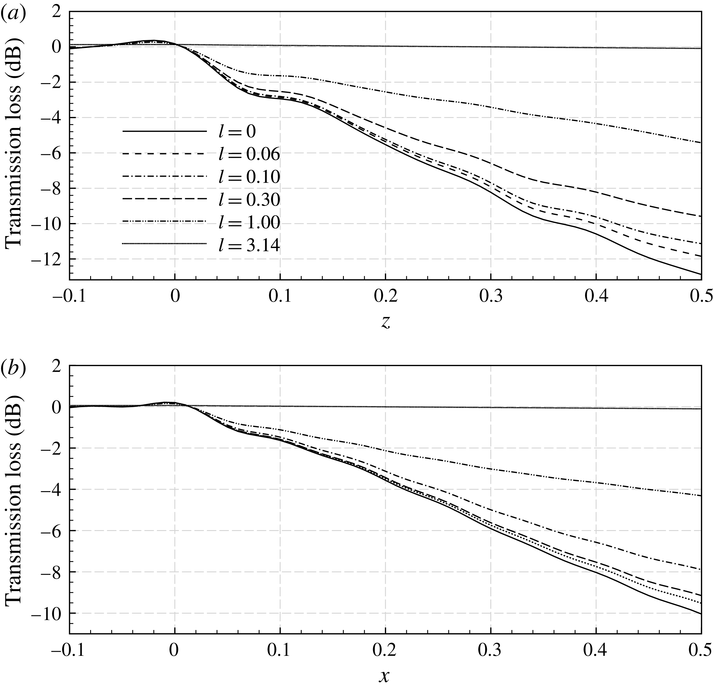
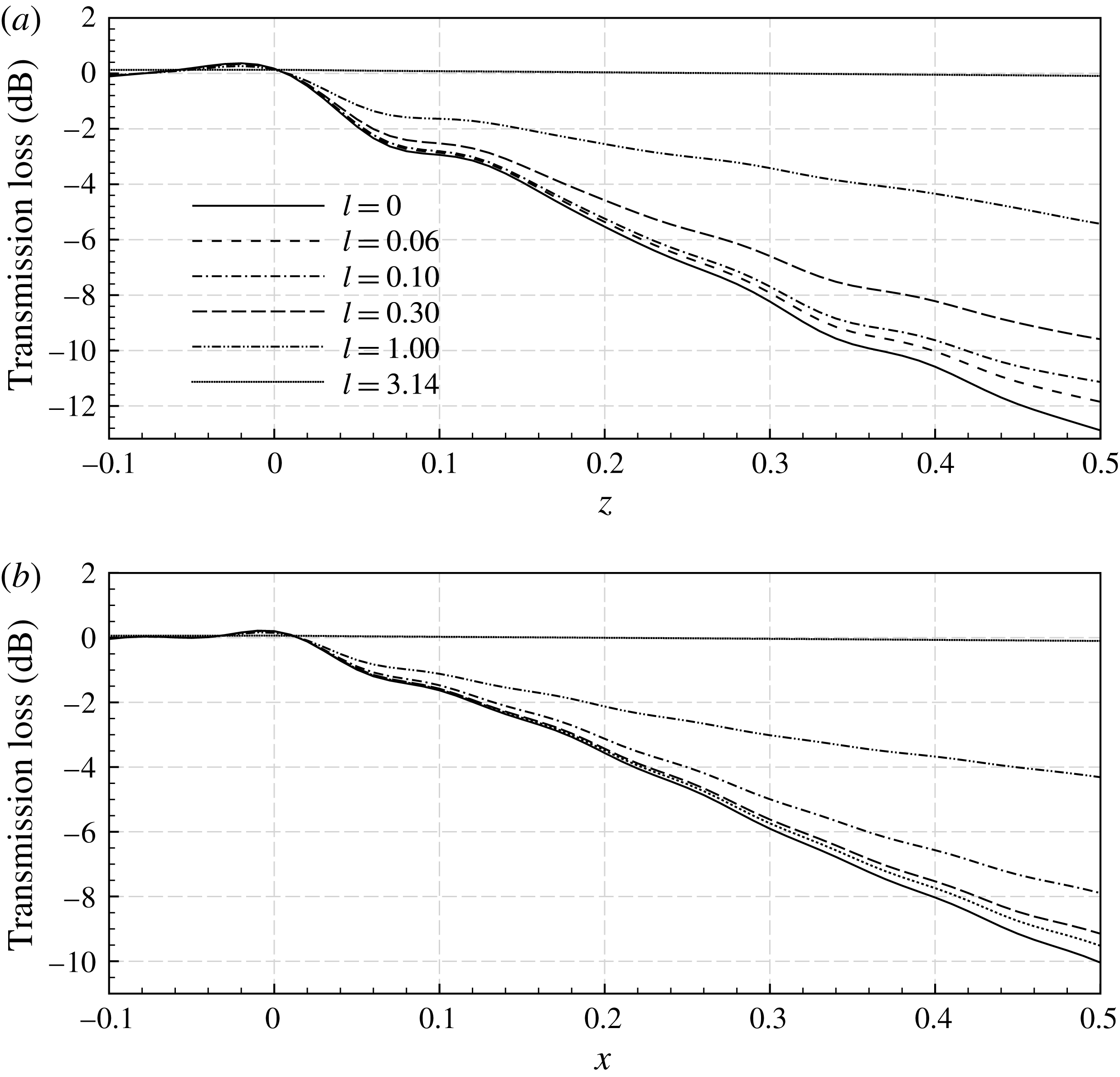
After validating the proposed model, we are able to produce predictions for various case set-ups rapidly. Figure 11 shows the axial distributions of transmission loss for the lined splices with different width. It is not surprising that a wider splice (e.g. with
 $l=0.3$
and
 $l=1.0$
) would lead to a smaller transmission loss. On the other hand, we can still identify the negative effect of the rigid splices even at
 $l=0.06$
, which is already much smaller than the corresponding wavelength in the
 ${\it\theta}$
direction. The theoretical model proposed in this work could easily explain this seemingly strange issue. The appearance of the rigid splices would scatter new azimuthal modes in addition to the modes of incident waves, even for the sub-wavelength splices. These new azimuthal modes will satisfy the famous Tyler–Sofrin selection rule, which is theoretically given by (2.23)–(2.24) in our model. It is easy to see that the scattered sound waves of the lower azimuthal modes are more prone to cut-on and would be less attenuated by the lining surface.
4. Summary
In this paper, we have developed a theoretical model for sound scattering from a semi-infinite lined duct with subsonic uniform flows and axially running rigid splices. The problem has been studied using the Wiener–Hopf method, which is usually preferable for its mathematical rigour and elegance. The key achievement of our work is the analytical description of axial liner splices using Fourier series expansions, which results in a complicated Wiener–Hopf matrix kernel of infinite size. After some appropriate approximation and truncations, the related Wiener–Hopf equation can be solved using typical routines for ordinary scalar kernels.
The proposed theoretical model has been demonstrated here in various case studies with representative set-ups. Both qualitative and quantitative studies have been conducted in this work. The mode selection due to the number of liner splices has been clearly elucidated using our theoretical model. Therefore, the analytical solutions should be able to help us to illuminate the inherent acoustic mechanisms and noise control effects of axially running, rigid liner splices.
The most essential concept is to represent circumferentially periodic scattered fields and liner splices using Fourier series expansions, and to establish the relations between these Fourier series within the framework of the Wiener–Hopf method. Then, given a circumferential layout of rigid splices, the corresponding Fourier coefficients would be found and all the rest can be straightforwardly solved. The whole theoretical development is (slightly) complicated but (largely) rigorous. The approximations that we have to make for our theoretical model are summarised here: (1) the impedance value of the rigid splices has to be finite to satisfy the Dirichlet condition; (2) the infinite Fourier series has to be truncated in the follow-up numerical implementation; and (3) the kernel matrix has to be approximated to enable an effective factorisation that was originally developed for scalar kernel cases. In addition, the Wiener–Hopf method requires semi-infinite boundary conditions, and thus cannot deal with liner splices of finite length, for which either mode matching method or numerical solvers should be considered.
Nevertheless, the concept behind this theoretical development is highly innovative, which significantly extends the current capability of the Wiener–Hopf method for duct radiation and scattering studies. Overall, the treatment by incorporating Fourier series and the Wiener–Hopf method is generic and should be applicable to problems with circumferentially varying impedance as well. Hence, our theoretical model should be beneficial for a host of new problems.
Acknowledgements
This work is partly supported by the National Science Foundation of China (Grant 11322222). In addition, during this research, the second author received his studentship from the Chinese Aeronautical Establishment Shanghai, and the third author received the Newton Advanced Fellowship from the Royal Society (ref. NA14081).