1 Introduction
The displacement of two miscible fluids in a porous medium is characterised by spreading and dilution (Kitanidis Reference Kitanidis1994). The former is a measure of the spatial extent of the solute plume, while the latter is a synonymous of mixing and refers to the increase in volume of fluid occupied by the solute (Le Borgne et al. Reference Le Borgne, Dentz, Bolster, Carrera, de Dreuzy and Davy2010). In this context, spreading is associated with an advective process and originates from fluid velocity variations at the pore scale (Illangasekare, Frippiat & Fucik Reference Illangasekare, Frippiat, Fucik, Thibodeaux and Mackay2011). This ‘differential advection’ process creates a distortion of the solute plume that (at some scale) is smoothed out by diffusion and local dispersion, which thus contribute to mixing. Although spreading and mixing are intimately related, it follows almost intuitively that a clear distinction among these two transport mechanisms is necessary when the length (or time) scales over which they are acting are significantly different. While this has been shown to be certainly the case for field-scale settings, where large structural and flow heterogeneities occur (Dentz et al. Reference Dentz, Le Borgne, Englert and Bijeljic2011), it is becoming increasingly apparent that such distinction is equally important to understand miscible displacements in laboratory rock samples (Bijeljic, Mostaghimi & Blunt Reference Bijeljic, Mostaghimi and Blunt2011). The latter are the subject of this study and represent a challenging scenario, because the scale of heterogeneity of key transport parameters (e.g. permeability) in these systems is often similar in order as the size of the system itself (Pini & Benson Reference Pini and Benson2013). The miscible displacement of oil by solvent injection in deep sedimentary formations as part of an enhanced oil recovery operation or the mixing between fresh and CO2-saturated brines during the geological storage of CO2 are just a few practical examples where a detailed understanding is required of flow and transport of solutes in rocks.
1.1 Laboratory observations of miscible displacements in reservoir rocks
In the laboratory, miscible displacements are traditionally studied by means of unidirectional tracer tests in cylindrical packs or cores and by matching the tracer effluent history (i.e. the breakthrough curve, BTC) with a solution of the so-called advection–dispersion equation (ADE). The latter treats the dispersion term as a Fickian diffusive flux associated with the longitudinal component of the hydrodynamic dispersion coefficient, which is further assumed to be independent of the concentration (Dullien Reference Dullien1992). With reference to the discussion above, it follows that such an approach works under the tacit assumption that the combined processes of spreading and mixing can be described with a single dispersion coefficient (Kitanidis Reference Kitanidis1994; Berkowitz, Scher & Silliman Reference Berkowitz, Scher and Silliman2000). Systems that fulfil this condition are random bead or sand packs, where the injected tracer plume develops in the form of a Gaussian shape; the latter can be fully described by a dispersion coefficient that is constant in space and time and that depends solely on the particle diameter (Perkins & Johnston Reference Perkins and Johnston1963). Moreover, when advection dominates over diffusion, this dispersion coefficient is found to increase linearly with the average pore fluid velocity (
 $D_{L}={\it\alpha}_{L}v$
) (Bear Reference Bear1972). The proportionality constant is given here by the so-called longitudinal dispersivity,
 ${\it\alpha}_{L}$
, which can therefore be regarded as an intensive property of the porous medium (Illangasekare et al.
Reference Illangasekare, Frippiat, Fucik, Thibodeaux and Mackay2011). In comparison to unconsolidated systems, the study of spreading and mixing in reservoir rock cores is more recent, although early investigators did recognise that the complex pore structure of rocks complicates considerably the analysis of these experiments (Scheidegger Reference Scheidegger1974). While we acknowledge that it represents a small fraction of what is admittedly a huge research field, we have intentionally limited the brief review that follows to experimental observations of BTCs made on reservoir rock cores, the latter being the main focus of this study.
The common perception is that rock samples possess dispersion coefficients that are larger than those expected from the sole effect of particle (i.e. grain) size. So-called ‘inhomogeneity factors’ have been introduced to account for this increased dispersivity when using the Fickian advection–dispersion model described above (Brigham, Reed & Dew Reference Brigham, Reed and Dew1961; Perkins & Johnston Reference Perkins and Johnston1963). Not surprisingly, this empirical approach seems to work only in a limited number of instances (Honari et al. Reference Honari, Bijeljic, Johns and May2015), while for most consolidated systems only a poor fit of the tracer elution history is achieved (Donaldson, Kendall & Manning Reference Donaldson, Kendall and Manning1976; Baker Reference Baker1977). In those cases, the term ‘non-Fickian’ (or anomalous) dispersion is adopted to refer to the characteristic asymmetry and long-time tailing of the tracer effluent profiles measured from pulse-tracer tests during core floods (Dullien Reference Dullien1992). To capture these effects, some authors have used dispersivity coefficients that increase with the distance travelled (Barry & Sposito Reference Barry and Sposito1989; Walsh & Withjack Reference Walsh and Withjack1994), while others have invoked new physical mechanisms, such as the mass transfer between the flowing fluid and a given fraction of the pore volume that is assumed to be immobile (Coats & Smith Reference Coats and Smith1964). The latter is often referred to as the ‘capacitance model’ and has found widespread use particularly in the petroleum literature (Donaldson et al. Reference Donaldson, Kendall and Manning1976; Baker Reference Baker1977; Bretz & Orr Jr Reference Bretz and Orr1987; Grattoni et al. Reference Grattoni, Rosen, Chertcoff and Bidner1987; Honari et al. Reference Honari, Bijeljic, Johns and May2015). The fact that structures where fluid stagnates are not readily found in many sandstones has led to the acknowledgment that anomalous transport in rock samples may instead originate from macroscopic heterogeneities, i.e. from the presence of regions with significantly different pore structures and, accordingly, permeability values on a length scale of the order of millimetres (Coats & Smith Reference Coats and Smith1964; Gist et al. Reference Gist, Thompson, Katz and Higgins1990; Walsh & Withjack Reference Walsh and Withjack1994). With analogy to field observations, the term ‘macrodispersion’ is applied in such cases to emphasize that the ‘differential advection’ process associated with these heterogeneities takes place at a scale larger than the characteristic size of a pore or a grain (Steefel & Maher Reference Steefel and Maher2009). By incorporating the effects of local fluctuations in the permeability, mathematical models were able to confirm that ‘non-Fickian’ anomalies (e.g. the long-time tailing) in rock samples can indeed be of advective origin (Charlaix & Gayvallet Reference Charlaix and Gayvallet1991).
1.2 Advanced reservoir core analyses with imaging techniques
In the methods presented above the rock sample has always been treated as being ‘uniformly heterogeneous’: although heterogeneities are accounted for in the modelling, whether through pockets of stagnant fluid or permeability fluctuations, these are assumed to be uniformly distributed throughout the sample. Sedimentary rocks are known to exhibit heterogeneities on a variety of scales reaching correlation lengths comparable to the size of a typical core sample (Murphy et al. Reference Murphy, Roberts, Yale and Winkler1984). Neglecting the detailed geometry of these heterogeneities within the sample precludes the unambiguous identification of the mechanisms of dispersion and results in the estimation of apparent transport parameters, which are inherently of limited predictive value. The fact that solute transport in Berea sandstone samples has been described through both ‘Fickian’ (Baker Reference Baker1977; Hulin & Plona Reference Hulin and Plona1989; Gist et al. Reference Gist, Thompson, Katz and Higgins1990) and ‘non-Fickian’ (Grattoni et al. Reference Grattoni, Rosen, Chertcoff and Bidner1987; Walsh & Withjack Reference Walsh and Withjack1994; Cortis & Berkowitz Reference Cortis and Berkowitz2005) approaches supports this observation. In this context, the use of multidimensional imaging techniques has been proposed to complement the analysis of tracer breakthrough curves for studying the transport of solutes in porous media. These techniques have greatly expanded the value of ‘reservoir core analysis’ since the early days (Wellington & Vinegar Reference Wellington and Vinegar1987; Withjack Reference Withjack1988) and experimental protocols are now available that enable the detailed quantification of the spatial variability of various physical properties of rocks, such as porosity and permeability, non-destructively (Krause, Perrin & Benson Reference Krause, Perrin and Benson2011; Krause, Krevor & Benson Reference Krause, Krevor and Benson2013; Pini & Benson Reference Pini and Benson2013). In comparison, the dynamic imaging of transport parameters is lagging due to the intrinsic difficulty with carrying out these measurements without disturbing the flow field. X-ray computed tomography (CT) (Walsh & Withjack Reference Walsh and Withjack1994; Fourar & Radilla Reference Fourar and Radilla2009) requires large concentrations of tracers (typically an iodine compound) to achieve sufficient density contrast for imaging that could lead to unwanted chemistry and/or buoyancy effects. Similarly, the presence of paramagnetic (e.g. clays, pyrite) or even ferromagnetic minerals (e.g. hematite) that are commonly found in rocks or soil samples can cause severe images artefacts on data obtained by magnetic resonance imaging (MRI) or nuclear magnetic resonance (NMR) methods and quantitative interpretation remains challenging (Guillot et al. Reference Guillot, Kassab, Hulin and Rigord1991; Greiner et al. Reference Greiner, Schreiber, Brix and Kinzelbach1997; Gladden & Mitchell Reference Gladden and Mitchell2011). On the contrary, studies using radioisotopes have shown that a minimal amount of tracer can produce sufficient activity to monitor its distribution in an opaque porous sample (Josendal, Sandiford & Wilson Reference Josendal, Sandiford and Wilson1952; Grattoni et al. Reference Grattoni, Rosen, Chertcoff and Bidner1987). These early measurements were however severely limited in the spatial resolution and only recently positron emission tomography (PET) has (re)emerged to fill this gap, by combining the benefits of multidimensional tomographic imaging with those related to the characteristic radiation of positron-emitting isotopes (Goethals et al. Reference Goethals, Volkaert, Jacobs, Roels and Carmeliet2009). With relevance to the present work, PET has been used to study the porosity of rock samples (Degueldre et al. Reference Degueldre, Pleinert, Maguire, Lehman, Missimer, Hammer, Leenders, Böck and Townsend1996; Maguire et al. Reference Maguire, Missimer, Emert, Townsend, Dollinger and Leenders1997) and to image transport in sediments (Khalili, Basu & Pietrzyk Reference Khalili, Basu and Pietrzyk1998) and sandstones (Ogilvie, Orribo & Glover Reference Ogilvie, Orribo and Glover2001). However, with the avowed intention of demonstrating the potential of PET to visualize fluid pathways inside porous samples, most studies so far have been largely qualitative, and the use of this technique for quantitative analyses is just beginning (Gründig et al. Reference Gründig, Richter, Seese and Sabri2007; Boutchko et al. Reference Boutchko, Rayz, Vandehey, O’Neil, Budinger, Nico, Druhan, Saloner, Gullberg and Moses2012; Fernø et al. Reference Fernø, Gauteplass, Hauge, Abell, Adamsen and Graue2015).
1.3 Modelling of solute transport in porous rocks
Various theories have been developed to model non-Fickian transport in heterogeneous porous media that have found widespread application in the context of (stochastic) subsurface hydrology. Both extensive (e.g. Berkowitz et al.
Reference Berkowitz, Cortis, Dentz and Scher2006) and brief (e.g. Dentz et al.
Reference Dentz, Le Borgne, Englert and Bijeljic2011) literature reviews are available where these theories are presented and discussed. Again, we shall restrict our discussion to their evaluation in the context reservoir core analyses. The continuous-time random walk (CTRW) theory appears to be the most general formalism to describe dispersive processes in geological formations. In fact, other successfully adopted formulations, such as the multi rate mass transfer approach (e.g. Haggerty, McKenna & Meigs Reference Haggerty, Mckenna and Meigs2000), the fractional advection dispersion equation (FADE, e.g. Benson, Wheatcraft & Meerschaert Reference Benson, Wheatcraft and Meerschaert2000) and, obviously, the classic ADE, have been shown to be special cases of this theory (Berkowitz et al.
Reference Berkowitz, Cortis, Dentz and Scher2006). CTRW does not rely on the assumption of Fickian transport; rather, it calculates a BTC based on a stochastic approach that uses a probability density function to describe (solute) particle transitions in space and time. While this function effectively maps solute movement to the underlying medium heterogeneity, its explicit connection to known physical information (e.g. to a spatial distribution of permeability within a rock sample) remains an area under development (Berkowitz et al.
Reference Berkowitz, Cortis, Dentz and Scher2006). As with any other probabilistic approach, computed quantities (e.g. the tracer concentration) are ensemble averaged and the method is therefore best utilized when the scale of heterogeneity is significantly smaller than the system size (Levin & Berkowitz Reference Levy and Berkowitz2003). In the context of rocks, CTRW has been validated by means of network models computed on reconstructed cubic samples of a Berea sandstone (Bijeljic & Blunt Reference Bijeljic and Blunt2006) and of a Portland limestone (Bijeljic et al.
Reference Bijeljic, Mostaghimi and Blunt2011) with side length of a few mm, which corresponds to 10–20
 $\times$
the characteristic length of heterogeneity at this scale. With the exception of one study using a 30-in. long Berea sandstone sample (Scheidegger Reference Scheidegger1974 revisited in Cortis & Berkowitz Reference Cortis and Berkowitz2005), CTRW has not been applied to describe transport in rock samples used for routine core analyses.
Approaches that are based on streamtube formulations belong also to the realm of stochastic hydrology and have been widely adopted to describe transport in heterogeneous porous media (Simmons, Ginn & Wood Reference Simmons, Ginn and Wood1995; Thiele, Rao & Blunt Reference Thiele, Rao and Blunt1996). These include among others the stochastic-advective (Ginn, Simmons & Wood Reference Ginn, Simmons and Wood1995) and the advective–dispersive streamtube (Cirpka & Kitanidis Reference Cirpka and Kitanidis2000; Ginn Reference Ginn2001) approach. These methods consider transport to take place in an ensemble of one-dimensional (1-D) streamtubes with individual constant velocities, instantaneous lateral intrastreamtube mixing and zero interstreamtube mixing. Transport in each streamtube is modelled by the 1-D ADE with a longitudinal dispersion coefficient, although in early formulations the latter was neglected (Simmons et al. Reference Simmons, Ginn and Wood1995). The method is built on the premise that Fickian transport behaviour holds at some (microscopic) scale, while spreading of the plume caused by heterogeneities is captured through the different streamtube velocities (e.g. permeability values) (Ginn Reference Ginn2001). The practicality of the method lies in the adoption of a mechanistic view of the porous medium, which is discretised into elements associated with averaged (volumetric) properties (e.g. porosity and permeability) that are directly accessible experimentally (Berkowitz et al. Reference Berkowitz, Cortis, Dentz and Scher2006). It is referred to as ‘stochastic’, because it uses a probability density function to represent the distribution of streamtube travel times resulting from the underlying medium heterogeneity. This function can be estimated from the deconvolution of a conservative tracer test or from a velocity field computed on a given realisation of the porous medium in terms of e.g. a random permeability field (Yabusaki, Steefel & Wood Reference Yabusaki, Steefel and Wood1998). With few exceptions (Thiele et al. Reference Thiele, Rao and Blunt1996), streamtube formulations have been applied to compute a BTC without any specific knowledge of the spatial distribution of velocities. Accordingly, to our knowledge, no comparison has been attempted between model results and the measured temporal and spatial evolutions of a full migrating plume. We anticipate that, in the context of reservoir core analyses, a deterministic computation of streamtube travel times could in principle be achieved and validated, because of the high resolution at which properties, such as permeability and solute concentration, can nowadays be measured in the laboratory by means of non-invasive imaging techniques (Krause et al. Reference Krause, Perrin and Benson2011, Reference Krause, Krevor and Benson2013; Pini & Benson Reference Pini and Benson2013).
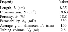
Properties of the Berea sandstone sample used in this study. The tubing volume is the total dead space between the input/output detectors and each face of the sample. Porosity has been obtained by X-ray CT scanning and the permeability (to water) is an average value from measurements reported in a previous study (Pini & Benson Reference Pini and Benson2013).

In this study, we investigate hydrodynamic dispersion during miscible displacements in a Berea sandstone sample by means of pulse-tracer tests. Experiments have been carried out while simultaneously imaging the whole rock sample by [11C]PET to provide quantitative information on the full spatial and temporal evolution of the migrating tracer plume. Multidimensional maps of the tracer concentration in the rock sample have been obtained with a spatial resolution of approximately 10 mm3 and provide evidence for macrodispersion effects caused by the presence of heterogeneities at the same scale. An advective–dispersive streamtube model is applied to describe solute transport. To this aim, the spatial distribution of streamtubes velocities is estimated from a subcore-scale permeability map of the rock sample that was obtained in an independent experiment. Matching the BTCs is used to make small adjustments to the original permeability map to provide a best fit to the effluent data. The refined permeability model is then used to predict the internal tracer concentration profile to be compared with the independent PET measurements of the full migrating plume. The benefits of in situ imaging for the study of mixing and spreading in porous media are highlighted and a discussion is presented on the necessity of such an approach for reservoir core analyses.
2 Experimental
2.1 Radiotracer solution
The active component of the radiotracer used in this study is the radionuclide
 $^{11}$
C with a half-life
 $t_{1/2}=20.33$
min. The isotope was produced in the chemical form of [11C]CO2 using a CTI-Siemens RDS111-11 MeV cyclotron located at the Biomedical Isotope Facility of the Lawrence Berkeley National Laboratory (Berkeley, CA, USA) and was subsequently released in an aqueous sodium bicarbonate solution ([11C]NaHCO3, 55 mM) (Vandehey & O’Neil Reference Vandehey and O’Neil2014). The latter constitutes the radioactive solution to be injected during the pulse-tracer experiments. An equivalent (non-labelled) NaHCO3 aqueous solution was used to saturate the core sample and as the background carrier fluid throughout the experimental campaign.
2.2 Rock sample and permeability heterogeneity
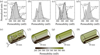
The properties of the Berea sandstone (Cleveland Quarries, Ohio, USA) core used in this study are summarised in table 1. A key feature of this specific sample is that its subcore-scale permeability distribution is precisely known at a resolution of a few mm3; the latter was obtained in a previous study (Pini & Benson Reference Pini and Benson2013) and is again shown in figure 1(a) together with the histogram plot of the corresponding permeability values. Notably, the distribution of permeability values at the subcore scale is relatively wide (200–500 mD, measured average permeability
 $k_{m}=330$
mD) and is bimodal, with approximately 25 % of the voxels belonging to fine-textured (and less permeable) strata that can be readily recognised in the three-dimensional (3-D) permeability map. Although Berea sandstone is the archetype of a well sorted and homogeneous rock, the presence of these characteristic layers has been reported in earlier studies (Brooks & Corey Reference Brooks and Corey1964). The latter are not readily noticeable in the dry or fully saturated state, but introduce fine-scale (mm–cm) variations in the permeability, whose effects have been shown to greatly influence fluid flow for both single (Walsh & Withjack Reference Walsh and Withjack1994) and multiphase (e.g. gas–water) systems (Perrin & Benson Reference Perrin and Benson2010; Krause et al.
Reference Krause, Perrin and Benson2011).
Multidimensional reconstructions of the Berea sandstone core used in this study in terms of permeability maps together with their corresponding histograms. (a,e) ‘Original’ reconstruction obtained from a laboratory characterisation study (Pini & Benson Reference Pini and Benson2013). In the histogram, the curves are normal distributions representing three subfamilies of voxels (dashed lines) and their contribution to the whole population of values (solid line). Three additional maps have been derived from (a,e), namely (b,f) ‘streamtubes’, (c,g) ‘tuned streamtubes’ and (d,h) ‘two layer’ (2P-ML). Voxel size: for all maps, (
 $x\times y$
)
 $=$
(2
 $\times$
2) mm2, while
 $z=3$
mm for (a) and 83.5 mm for (b–d). Additional details are given in § 2.2.

An empirical semivariogram was calculated to investigate the correlation structure of the voxel permeability values in the
 $x,y,z$
directions by using the following equation:
 $$\begin{eqnarray}\hat{{\it\gamma}}_{i}(h)=\frac{1}{2N(h)}\mathop{\sum }_{N(h)}(w_{j}-w_{l})^{2},\end{eqnarray}$$
where the subscript
 $i$
refers to the direction used for calculating the variogram (
 $i=x$
,
 $y$
or
 $z$
),
 $h$
is the lag (i.e. the distance separating two voxels),
 $N$
is the set of all pairwise distances (
 $j-l=h$
) and
 $w_{j}$
and
 $w_{l}$
are data values at spatial locations
 $j$
and
 $l$
, respectively. Note that (2.1) was applied on the log-transformed data,
 $w=\log _{10}(k)$
, because the latter follow a normal distribution with location and scale parameter given by
 ${\it\mu}=2.52$
and
 ${\it\sigma}=0.0715$
, respectively, as shown in figure 2(a). The computed variograms are plotted in figure 2(b), together with predictions from an exponential model that was used to match the experimental data (Sarma Reference Sarma2009),
 $$\begin{eqnarray}{\it\gamma}_{i}(h)=(C_{i}-{\it\gamma}_{i}^{0})\left[1-\text{exp}(-3h/a_{i})\right]+{\it\gamma}_{i}^{0},\end{eqnarray}$$
where
 $C={\it\gamma}(h\rightarrow \infty )$
is the sill (i.e. the limiting value of the variogram),
 $a$
is the range (i.e. the distance at which the sill is reached and the data are no longer autocorrelated) and
 ${\it\gamma}^{0}={\it\gamma}(h=0)$
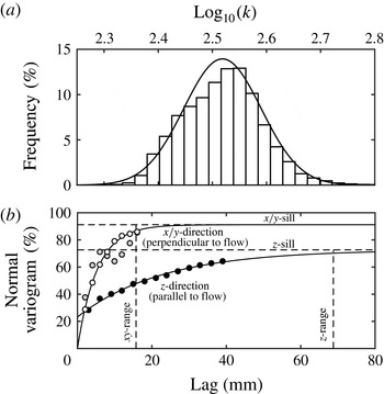
represents the so-called nugget effect. It can be seen from the plot that the correlation length in the
 $z$
-direction (parallel to flow) is much larger than either value obtained in the
 $x/y$
-direction, with the value of the range being just below the sample length (
 $a_{xy}\approx 1.5~\text{cm}<a_{z}\approx 7~\text{cm}~\approx L$
). The sill in the
 $x/y$
-direction is also the largest (and close to the variance of the whole distribution), suggesting that permeability heterogeneity in this sample may be primarily attributed to variations on this plane. These results again confirm the presence of those textural features that are characteristic of Berea sandstone and that are readily visible in figure 1(a,e) as layers running parallel to the direction of flow. As explained below, these observations are used to justify the simplification of the original voxel permeability map into an ensemble of streamtubes with constant permeability.
Statistics of the voxel permeability map of the Berea sandstone sample used in this study and shown in figure 1(a,e). (a) Histogram plot of the log-transformed voxel permeability values together with a normal distribution probability density function (PDF) curve (
 ${\it\mu}=2.52$
,
 ${\it\sigma}=0.0715$
). (b) Computed empirical semivariograms (symbols) in the
 $x$
,
 $y$
and
 $z$
directions. The variograms are computed using (2.1) and normalised with the variance of the log-transformed permeability distribution. The curves are best matches obtained from an exponential variogram model (2.2); the values of the fitted parameters are as follows:
 $C_{z}=0.0037$
,
 $C_{y}=0.0047$
,
 $a_{z}=68.8$
mm,
 $a_{y}=15.8$
mm,
 ${\it\gamma}_{z}^{0}=0.0012$
,
 ${\it\gamma}_{y}^{0}=0$
.

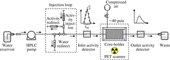
Schematic of the experimental apparatus used for the pulse-tracer experiments with simultaneous PET imaging.

With the intent of investigating the role of permeability heterogeneity on miscible displacements, four permeability maps are considered in this study that are derived from the original (experimental) map. These include a single-permeability (homogeneous) case, together with other three scenarios shown in figure 1(b–d, f–h) as 3-D reconstructions of the rock sample. Histograms are shown on top of each map to represent the corresponding distribution of permeability values. Map (b,f) reproduces the permeability field with parallel ‘streamtubes’ that have been obtained by taking the harmonic average of the original voxel permeability values in (a) along the longitudinal axis of the sample. For map (c,g), ‘tuned streamtubes’ have been obtained from (b,f) by further multiplying by a factor of 0.91 and 1.015 the streamtubes’ permeability values that are found below and above a threshold value of 285 mD, respectively. The values of these parameters were selected so as to attain a best match to the tracer effluent curve measured in one tracer test and were then used throughout the study. This is somewhat analogous to the procedure adopted in the stochastic advective–dispersive streamtube approaches (Cirpka & Kitanidis Reference Cirpka and Kitanidis2000; Ginn Reference Ginn2001) to obtain a distribution of streamtube travel times (i.e. velocities), with the difference that in our case their spatial arrangement is not free, but determined by the experimental permeability map. The major effect of such ‘tuning’ is that the range of streamtube permeability values is slightly stretched and reproduces more closely the one observed in the original voxel permeability map (figure 1 a,e), when the two main families of voxels are considered (90 % of the entire population). Finally, map (d,h) reduces the complexity of map (c) by using only two representative permeability values, while maintaining a similar spatial pattern as in (a,e). We refer to this scenario as ‘2P-ML’ to emphasise that two different values of permeability appear in multiple parallel layers. It is worth noting that each map possess the same average permeability of 330 mD that was determined from laboratory experiments.
2.3 Apparatus
The pulse-tracer experiments were performed using the experimental set-up depicted in figure 3. The core holder (Larson Engineering, Boulder, CO, USA) can accommodate a cylindrical sample of 5 cm in diameter and of variable length. The sample is positioned between two Delrin® end-caps, which have circular grooves to distribute the fluid over its entire cross-sectional area. Compressed air provides a confining annular pressure between the jacketed sample and an outer 1.5 mm-thick aluminium tube (internal diameter (ID) 7 cm), so as to prevent bypass flow during the experiments. In addition, four all-thread rods secure the assembly and ensure good contact between the sample and the edges of the end caps. The core holder is placed horizontally on the bed of the scanning instrument (Siemens Biograph 6 PET/CT scanner with a 80 cm ring diameter and 4 mm detector element width) and is connected to two shielded detectors (miniature Si PIN diode detectors, Carroll-Ramsey and Associates, USA) that monitor the activity of the fluid entering and leaving the sample at 5 s intervals. The cumulative void volume between the sample and the detectors is approximately 3 ml and its exact value has been found by matching the mean residence time of the measured effluent tracer profile to the expected average residence time with the given flow rate and rock’s pore volume (see table 1). A displacement pump (Waters, Model 590 HPLC) is used for continuous injection of the carrier fluid through the sample at controlled flow rates (1.4 or
 $3.4~\text{ml}~\text{min}^{-1}$
in this study). A loop consisting of four syringes is used to inject the tracer and allows diverting the flow of the background fluid during injection of the tracer, so as to maintain a constant total volumetric flow rate through the sample. This generates a radiotracer input function with the shape of an isosceles triangle that can be easily reproduced for modelling purposes. The various components the system are connected by means of PEEK and PTFE tubing (with OD 1/16”–1/8”).
2.4 Experimental procedure and PET imaging
All experiments have been carried out at room temperature and ambient pressure conditions. To ensure a tight annular seal around the sample, the latter was wrapped with a 3 mm thick sheet of soft rubber gasket material that was fixed with PTFE thread-sealer tape; three o-rings were additionally placed along the length of the wrapped core and held by means of an outer heat-shrinkable Teflon layer. Care was taken to maintain the same orientation of the sample as for the 3-D permeability map shown in figure 1. After mounting the jacketed sample in the core holder and placing it on the bed of the scanner, the confining pressure on the sample was increased and set to a value of approximately 40 psia. The system was then purged with gaseous CO2, followed by the injection of the aqueous background solution that was circulated for various pore volumes, so as to dissolve any remnant CO2. After that, a X-ray scan of the entire core sample was taken to register its position. Each pulse-tracer experiment consisted of the injection of a bolus (
 ${\sim}$
3.5 ml) of the radioactive solution ([11C]NaHCO3 at 55 mM) with an activity concentration of approximately 1 mCi (37 MBq), while keeping a constant volumetric flow through the sample. While the term ‘activity concentration’ represents the correct notation for measurements with radionuclides (in
 $\text{mCi}~\text{ml}^{-1}$
or
 $\text{Bq}~\text{ml}^{-1}$
), we are going to interpose the terms ‘activity’ and ‘concentration’ when describing the exact same property. For the sake of better clarity, the symbols
 $a$
(or
 $A$
) are used when referring to experimental results and
 $c$
(or
 $C$
) to model predictions.
For the entire duration of the experiment (30–60 min depending on the flow rate), the activity
 $a^{D}$
of the fluid entering and leaving the sample is measured and corrected to the radioactivity at the injection time
 $a_{0}^{D}$
by accounting for radioactive decay, i.e.
 $a_{0}^{D}(t)=a^{D}(t)\text{e}^{{\it\lambda}t}$
with
 ${\it\lambda}=\text{ln}(2)/t_{1/2}$
. Simultaneously, the whole axial field of view of the PET scanner (
 ${\sim}$
22 cm) is imaged and the corresponding tracer activity in the rock sample is detected. This information is converted into a 3-D image with a voxel dimension of
 $0.509~\text{mm}~\text{pixel}^{-1}$
by using the algorithm provided as part of the instrument’s reconstruction software package. For the PET scanner used in this study, the effective spatial resolution is expected to be
 ${\sim}$
2.5 mm at FWHM (Levy & Hoffman Reference Levin and Hoffman1999), and the reconstructed images will be analysed accordingly. The preparation of the PET data for subsequent analysis is completed by (i) resampling the data set into an (arbitrary) number of constant time frames
 ${\rm\Delta}t$
and by (ii) correcting the measured tracer concentration for radioactive decay. Mathematically, step (i) is expressed as follows:
 $$\begin{eqnarray}A_{j}^{PET}(t_{i})=\frac{1}{{\rm\Delta}t}\displaystyle \int _{t_{1}}^{t_{2}}a_{j}^{PET}(t)\,\text{d}t,\end{eqnarray}$$
where
 $A_{j}^{PET}(t_{i})$
is the average tracer activity in any given voxel
 $j$
over a time frame
 ${\rm\Delta}t$
, while
 $t_{1}=t-{\rm\Delta}t/2$
,
 $t_{2}=t+{\rm\Delta}t/2$
and
 $t_{i}=(t_{1}+t_{2})/2$
. Step (ii) requires accounting for the amount of decay during the selected image frame, i.e.
 $$\begin{eqnarray}\displaystyle DF(t_{i})=\frac{1}{{\rm\Delta}t}\int _{t_{1}}^{t_{2}}\text{e}^{-{\it\lambda}t}\,\text{d}t=\text{e}^{-{\it\lambda}t_{i}}\left(\frac{1-\text{e}^{-{\it\lambda}{\rm\Delta}t}}{{\it\lambda}{\rm\Delta}t}\right),\end{eqnarray}$$
with
 $DF(t_{i})=A_{j}^{PET}(t_{i})/A_{0j}^{PET}(t_{i})$
representing the decay factor. In deriving (2.4) we assume that radioactive decay is the sole mechanism affecting the tracer concentration during the time frame
 ${\rm\Delta}t$
. We note, however, that in this study
 ${\rm\Delta}t=1$
min and the term in brackets takes a value near unity (
 $0.983\approx 1$
); accordingly, the previous assumption can be relaxed and the decay-corrected tracer average activity in any given voxel
 $j$
is simply calculated as:
 $$\begin{eqnarray}A_{0j}^{PET}(t_{i})=\text{e}^{{\it\lambda}t_{i}}A_{j}^{PET}(t_{i}),\end{eqnarray}$$
where
 $A_{0j}^{PET}(t_{i})$
refers to a concentration measured at time
 $t_{i}$
and lumps together all events taking place over the time frame
 ${\rm\Delta}t=(t+{\rm\Delta}t/2)-(t-{\rm\Delta}t/2)$
. We also note that the selection of 1 min intervals represents a trade off between a temporal resolution that is useful for analysis and good image quality at the spatial resolution that is required in this study. The latter is significantly reduced when a small amount of radioactivity is injected, thus requiring sufficiently long ‘exposure’ when reconstructing the image frames. The obtained voxel activity values are reported in radioactivity concentration per unit voxel volume (
 $\text{mCi}~\text{ml}^{-1}$
or
 $\text{Bq}~\text{ml}^{-1}$
, as noted throughout the manuscript with
 $1~\text{mCi}=2.7027\times 10^{-8}~\text{Bq}$
).
3 Modelling
The transport of the tracer through the sample is described by the well-known ADE, which in 1-D form reads as follows:
 $$\begin{eqnarray}{\it\phi}\frac{\partial c}{\partial t}+u\frac{\partial c}{\partial z}={\it\phi}D_{L}\frac{\partial ^{2}c}{\partial z^{2}},\end{eqnarray}$$
where
 ${\it\phi}$
is the rock’s porosity,
 $c$
is the tracer concentration,
 $u$
is the constant superficial fluid velocity,
 $D_{L}$
is the longitudinal dispersion coefficient and
 $z$
and
 $t$
are the space and time coordinates. The superficial velocity is defined as
 $u=q/S={\it\phi}v$
, with
 $q$
,
 $S$
and
 $v$
being the volumetric flow rate, the sample cross-section and the interstitial (pore) fluid velocity, respectively. Note that transverse dispersion is neglected in this formulation. The longitudinal dispersion coefficient is defined as (Illangasekare et al.
Reference Illangasekare, Frippiat, Fucik, Thibodeaux and Mackay2011),
 $$\begin{eqnarray}D_{L}=D_{m}+{\it\alpha}_{L}v,\end{eqnarray}$$
where
 $D_{m}$
is an ‘effective’ molecular diffusion coefficient in the liquid and
 ${\it\alpha}_{L}$
is the longitudinal dispersivity. The former is likely to be smaller than the corresponding diffusivity in the bulk liquid,
 $\mathscr{D}\approx 1\times 10^{-5}~\text{cm}^{2}~\text{s}^{-1}$
, due to the tortuosity that characterises a porous medium (Dullien Reference Dullien1992). The experiments presented in this study have been carried out in the regime
 $Pe\approx 10{-}20$
, as estimated from the following formulation of the P
 $\acute{\text{e}}$
clet number:
 $$\begin{eqnarray}Pe=\frac{vd_{P}}{\mathscr{D}},\end{eqnarray}$$
where the grain diameter,
 $d_{P}$
, is used as the characteristic length scale. Under such conditions, the ratio between the dispersion and diffusion coefficient is expected to lie within the range
 $D_{L}/\mathscr{D}\approx 100{-}200$
, as reported in previous studies where Berea sandstone has been used (Hulin & Plona Reference Hulin and Plona1989; Gist et al.
Reference Gist, Thompson, Katz and Higgins1990). It follows that the second term in (3.2) is large enough that molecular diffusion can be neglected and
 $D_{L}\approx {\it\alpha}_{L}v$
. The well-known Danckwerts boundary conditions (Fogler Reference Fogler1999) are applied to solve (3.1):
 $$\begin{eqnarray}\displaystyle \left.\begin{array}{@{}c@{}}\displaystyle \text{for}~z=0:\quad c(z=0)=c_{F}+{\displaystyle \frac{{\it\phi}D_{L}}{u}}\left.{\displaystyle \frac{\partial c}{\partial z}}\right|_{z=0},\\ \displaystyle \text{for}~z=L:\quad \left.{\displaystyle \frac{\partial c}{\partial z}}\right|_{z=L}=0,\end{array}\right\} & & \displaystyle\end{eqnarray}$$
with
 $c_{F}$
being the tracer concentration in the tubing just outside the inlet face of the rock sample. The latter is given by a triangular radiotracer input function fitted to the activity measured by the inlet detector during injection:
 $$\begin{eqnarray}\displaystyle \left.\begin{array}{@{}c@{}}\text{for}~t<{\displaystyle \frac{t_{inj}}{2}}:\quad c_{F}={\displaystyle \frac{2c_{F}^{0}t}{t_{inj}}},\\ \text{for}~{\displaystyle \frac{t_{inj}}{2}}\leqslant t\leqslant t_{inj}:\quad c_{F}=2c_{F}^{0}\left(1-{\displaystyle \frac{t}{t_{inj}}}\right),\end{array}\right\} & & \displaystyle\end{eqnarray}$$
where
 $t_{inj}$
and
 $c_{F}^{0}$
represent the base and the tip of the tracer input function (see figure 2). Each experiment begins with the sample completely saturated with fresh (non-labelled) water and the initial condition for each simulation is defined as:
 $$\begin{eqnarray}\displaystyle \text{for}~t=0\quad \text{and}\quad 0\leqslant z\leqslant L:\quad c=0. & & \displaystyle\end{eqnarray}$$
3.1 Solution procedure
The partial differential equation (3.1) is discretised in space using the finite-difference method with 164 grid points corresponding to a constant width
 ${\rm\Delta}x=0.05$
cm. To this aim, the space derivatives are approximated using the central difference operator for each internal node and the backward difference operator for the first and last node. This produces a system of 164 ordinary differential equations (ODEs), which are solved simultaneously in time using the ode15s solver in MATLAB. The solver uses an implicit method for the numerical integration of the ODEs based on backward differences with a variable time step. The latter is chosen so that the local error
 $e_{i}$
in
 $c_{i}$
at each time step satisfies
 $|e_{i}|\leqslant r|c_{i}|+a_{i}$
. In this study, the relative (
 $r$
) and absolute (
 $a_{i}$
) error tolerances have been set to 0.01 % and
 $1\times 10^{-4}~\text{mCi}~\text{ml}^{-1}$
, respectively, while the maximum allowed time step was limited to 0.01 min. The input parameters used for the model are the sample properties listed in table 1. These are common to each experiment and modelling scenario considered, while the flow rate,
 $q$
, is adjusted depending on the experimental conditions. The longitudinal dispersivity
 ${\it\alpha}_{L}=D_{L}/v$
represents the sole fitting parameter, which was estimated for each experiment by reproducing the experimentally obtained tracer effluent profiles (i.e. the detector’s data) with the model described above, while minimising the following objective function:
 $$\begin{eqnarray}{\it\Phi}^{2}=\frac{1}{N_{P}}\displaystyle \mathop{\sum }_{j=1}^{N_{P}}\left(\frac{c_{j}^{out}-a_{0j}^{D}}{a_{0j}^{D}}\right)^{2},\end{eqnarray}$$
where
 $c^{out}$
is the flux-averaged effluent concentration predicted by the model, while
 $a_{0}^{D}$
is the decay-corrected activity concentration measured with the detector.
 $N_{P}$
is the number of experimental data points in the tracer effluent curve. The parameters of the input pulse function (
 $t_{inj}$
and
 $c_{F}^{0}$
) are summarized on the right of table 2 together with the corresponding amount of activity injected. A grid convergence analysis was carried out to quantify the error affecting the numerical solution of (3.1) by estimating the pulse breakthrough time,
 $t_{B}$
. The latter has been estimated as the time at which the derivative of the BTC takes a value of
 $2\times 10^{-3}~\text{mCi}~\text{ml}^{-1}~\text{min}^{-1}$
. The error is computed as
 ${\it\varepsilon}=(f_{160}-f_{i})/f_{160}$
, where
 $f_{160}$
represents the value of
 $t_{B}$
computed on a grid with 160 points and
 $f_{i}$
is the solution obtained when the grid is varied between 20 and 320 points. Results from this exercise show that the error takes a value of
 ${\it\varepsilon}=8.9$
, 0.6 and 0.2 % for
 $f_{i}=20$
, 40 and 120, and stabilises at a negligible level beyond that. Other measures, such as the first moment of the BTC, give a very similar trend, while a negligible error (
 ${<}0.1$
%) is observed in the material balance irrespectively of the grid refinement, thus confirming the accuracy of the simulations results presented below on a grid with 164 nodes.
Overview of the experiments conducted in this study. Reported variables are: volumetric flow rate (
 $q$
), average residence time (
 ${\it\tau}={\it\phi}AL/q$
), dose amount (
 $M_{exp}^{out}$
with corresponding error,
 ${\it\varepsilon}=1-M_{exp}^{out}/M_{exp}^{inj}$
) and mean residence time (
 $t_{R,exp}^{\ast }$
). Model parameters are: the tip (
 $c_{F}^{0}$
) and base (
 $t_{inj}$
) of the triangular tracer input function, and the simulated dose amount (
 $M^{out}$
with corresponding error,
 ${\it\varepsilon}$
).

3.2 Model scenarios
As anticipated above, three modelling approaches are considered in this study that differ in the level of characterisation of the rock sample in terms of permeability, namely the 1-D (homogeneous), the ‘streamtube’ and the ‘2P-ML’ model. For these last two cases, (3.1) is solved for each streamtube (
 $N_{K}=431$
) or layer (
 $N_{K}=2$
) and the average effluent tracer concentration is calculated as
 $c^{out}=\sum _{i=1}^{N_{K}}c_{i}q_{i}/q$
, with
 $c_{i}$
being the effluent concentration from streamtube (or layer)
 $i$
and
 $q_{i}$
its volumetric flow rate. The latter is related to the average flow rate
 $q$
through the relationship that describes Darcy’s flow in a system of parallel horizontal layers without cross-flow, i.e.
 $q_{i}/q=(S_{i}k_{i})/(Sk_{m})$
, with
 $S_{i}$
and
 $k_{i}$
being the cross-section and permeability of layer
 $i$
, respectively. For the ‘streamtube’ model the values of
 $k_{i}$
are known and
 $S_{i}$
is set by the scanner resolution (
 $S_{i}=4~\text{mm}^{2}$
in this study), while for the ‘2P-ML’ model
 $S_{i}$
is estimated based on the selected pairs of permeability values, i.e.
 $S_{1}/S=(k_{m}-k_{2})/(k_{1}-k_{2})$
and
 $S_{2}=S-S_{1}$
. It should also be noted that the total volumetric flow rate used in the streamlines scenario has been corrected to account for a cross-section of the sample (
 $S=431\times 0.04=17.24~\text{cm}^{2}$
) that is slightly smaller than the physical value reported in table 1.
A few remarks are warranted with respect to the application of the models that are based on streamtubes (or layers). First, in adopting the streamtube geometry we are assuming that the correlation length of the permeability in any direction perpendicular to flow is much smaller than the sample diameter; accordingly, the correlation length in the direction of bulk flow is at least as large as the sample length and the permeability within a streamtube is constant. As discussed in § 2.2 and shown in figure 2 this assumption is justified, as it reflects the characteristic structural features of the sample considered in this study. As to the underlying transport processes, the adopted formulation assumes that the solute in each streamtube undergoes longitudinal mixing and instantaneous lateral mixing within the streamtube, while mixing between streamtubes (e.g. transverse dispersion) is neglected. For the flow regime investigated in this study (
 $Pe\approx 10{-}20$
), the ratio between the longitudinal and transverse dispersion coefficient takes a value of
 $D_{L}/D_{T}\approx 35$
, as estimated from results reported in literature for Berea sandstone, i.e.
 $D_{L}/\mathscr{D}\approx 100{-}200$
(Hulin & Plona Reference Hulin and Plona1989; Gist et al.
Reference Gist, Thompson, Katz and Higgins1990) and
 $D_{T}/\mathscr{D}\approx 3{-}5$
(Bijeljic & Blunt Reference Bijeljic and Blunt2007), and in agreement with common observations for unconsolidated porous systems (Perkins & Johnston Reference Perkins and Johnston1963). We believe that these figures, together with the small scale of our experiment, support the approximation of negligible transverse dispersion, while the streamtube formulation allows resolving of the important mechanism of macrodispersion, i.e. the spreading of the tracer plume along distinct convective paths within the rock sample. Finally, irrespectively of the number of streamtubes, each scenario uses a single value for the dispersivity,
 ${\it\alpha}_{L}$
, while the dispersion coefficient in each streamtube changes according to its permeability, because
 $D_{L}=v{\it\alpha}_{L}$
. This approach ensures that the obtained results are consistent with observations from the literature that support this linear relationship for experiments where diffusion can be neglected (advection–dispersion control) (Perkins & Johnston Reference Perkins and Johnston1963; Illangasekare et al.
Reference Illangasekare, Frippiat, Fucik, Thibodeaux and Mackay2011).
3.3 Residence time, mass balance and concentration profiles
The concept of residence-time distribution (RTD) (Fogler Reference Fogler1999) is used to evaluate the results from the pulse-tracer tests. When applied to the effluent tracer profile predicted by the model, the RTD distribution function
 $E(t)$
is defined as
 $$\begin{eqnarray}E(t)=\frac{c^{out}(t)}{\displaystyle \int _{0}^{\infty }c^{out}(t)\,\text{d}t}.\end{eqnarray}$$
Accordingly, the denominator in (3.8) is used to compute the total amount of tracer produced, i.e.
 $$\begin{eqnarray}M^{out}=q\displaystyle \int _{0}^{\infty }c^{out}(t)\,\text{d}t\end{eqnarray}$$
while the first moment of the RTD function provides an estimate for the mean residence time
 $t_{R}$
, i.e.
 $$\begin{eqnarray}t_{R}=\displaystyle \int _{0}^{\infty }tE(t)\,\text{d}t.\end{eqnarray}$$
The integrals in (3.8)–(3.10) are computed via the trapezoidal method and are truncated at
 $t=60$
min for this study. The value of
 $t_{R}$
is corrected to account for the mean residence time of the tracer input function, i.e.
 $t_{R}^{\ast }=t_{R}-0.5t_{inj}$
, in order to be compared with the expected average residence time of the rock sample,
 ${\it\tau}={\it\phi}AL/q$
. Application of (3.9) to the injected tracer profile allows for a verification of the material balance by quantifying the error,
 ${\it\varepsilon}=1-M^{out}/M^{inj}$
. The exact same exercise is repeated for evaluating the experimental results and the corresponding parameters are calculated, namely
 $M_{exp}^{inj}$
,
 $M_{exp}^{out}$
and
 $t_{R,exp}^{\ast }$
. Note that in the latter case the computed mean residence time is additionally corrected for the amount of time (
 $t_{d}=V_{d}/q$
) that the tracer has spent in the tubings between the rock sample and the detectors. Finally, tracer concentrations computed within the rock are resampled over the time interval
 ${\rm\Delta}t=1$
min to allow for a direct comparison with the dynamic image frames generated from the PET scanner (see § 2.4), i.e.
 $$\begin{eqnarray}C(t_{i})=\frac{1}{{\rm\Delta}t}\displaystyle \int _{t_{1}}^{t_{2}}c(t)\,\text{d}t\end{eqnarray}$$
with
 $t_{2}-t_{1}={\rm\Delta}t$
. Note that when compared to those measured by PET (
 $A_{0j}^{PET}$
), the concentration values obtained from (3.11) need to be additionally multiplied by the porosity
 ${\it\phi}$
, as the former are reported per unit voxel volume.
4 Results
The first appraisal of the three pulse-tracer experiments is based on the results summarized in table 2. For each test, the total activity measured in the effluent stream,
 $M_{exp}^{out}$
, agrees with the corresponding input value,
 $M_{exp}^{inj}$
, within a margin of error of 8 % (
 $\pm$
0.1 mCi), after the correction for radioactive decay has been applied. Hereby, sources of unaccounted mass might be due to uncertainty in the numerical integration of the input pulse function. Nevertheless, the good mass recovery (
 ${>}90\,\%$
) suggests that the tracer can be regarded as conservative. Relative deviations smaller than 3 % are found between the mean residence time,
 $t_{R,exp}^{\ast }$
, that is calculated from the experimental RTD function (3.8) and the value,
 ${\it\tau}$
, that is predicted from the displacement of one pore volume of resident fluid. This result suggests that the volumetric flow across the system is constant and, accordingly, that stagnant zones are absent. In other words, a model of the form presented in § 3 that includes only the ADE should be sufficient to properly describe transport in Berea sandstone. The mean residence time is found to be inversely proportional to the flow rate, i.e.
 $q^{A}/q^{C}\approx t_{R,exp}^{\ast C}/t_{R,exp}^{\ast A}$
, thus further supporting the reliability of this experimental data set.
4.1 Tracer breakthrough curves
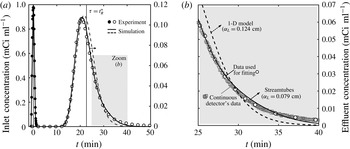
Figure 4 presents a set of results from test C and includes (i) a plot of the tracer concentration,
 $a_{0}^{D}(t)$
, as measured by activity detectors mounted upstream and downstream of the core sample (figure 4
a), together with (ii) a close-up of (a) over the time frame 25–40 min (figure 4
b). In the plots, the experimental data are represented by the symbols, while the lines are results from the homogeneous (1-D, dashed lines) and the ‘tuned streamlines’ model (solid lines). Two features are readily noticeable on the tracer breakthrough curve that are the direct manifestation of mechanical dispersion, namely the asymmetry of the concentration profile and the early peak at
 $t<{\it\tau}$
. Most importantly, it can be seen that the ‘tuned streamtubes’ model provides a better fit to the experimental data (
 ${\it\alpha}_{L}=0.079$
cm,
 ${\it\Phi}=12.3$
) as compared to the 1-D model (
 ${\it\alpha}_{L}=0.124$
cm,
 ${\it\Phi}=15.1$
). Results from an
 $F$
-test (Motulsky & Christopoulos Reference Motulsky and Christopoulos2003) confirm that the observed decrease in the value of the objective function
 ${\it\Phi}$
is statistically significant at
 $p=0.05$
(
 $F_{44,43}=9.5>F_{crit}=4,p=0.004$
). Such improvement can easily be seen in figure 4(b), where the ‘tuned streamtubes’ model follows more closely the slow decay of the measured tracer concentration and where the continuous readings of the activity detectors are also shown to emphasise the negligible noise in the experimental data set.
Results from a pulse-tracer experiment at
 $q=1.36~\text{ml}~\text{min}^{-1}$
(experiment C): (a) inlet and effluent concentration profiles (as measured by the activity detectors) as a function of time and (b) close-up of (a) over the time interval 25–40 min. Symbols represent experimental data and lines are simulation results obtained upon applying the homogeneous (1-D, dashed line,
 ${\it\alpha}_{L}=0.124$
cm) or the ‘tuned streamtube’ model (solid line,
 ${\it\alpha}_{L}=0.0790$
cm). For the fitting of the models to the experiments, the data shown as circles have been used that have been obtained from an interpolation of the detectors’ continuous readings (squares).

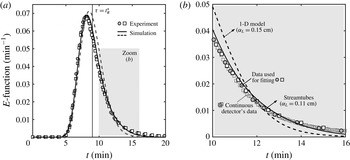
A similar set of results is shown in figure 5 for tests A and B, which have been carried out under identical experimental conditions. In the figure, the effluent tracer curve is plotted in terms of the RTD function,
 $E(t)$
(3.8), so as to account for the slightly different activity of tracer injected. It can be seen that the two sets of data (shown as square and circles in the plot) are in excellent agreement and confirm the repeatability of the experimental technique, in addition to the negligible noise in the measured activity concentration. Again, the ‘tuned streamlines’ model (
 ${\it\alpha}_{L}\approx 0.11$
cm,
 ${\it\Phi}\approx 17$
) outperforms the 1-D model (
 ${\it\alpha}_{L}\approx 0.16$
cm,
 ${\it\Phi}\approx 20$
) in capturing the behaviour of the tracer effluent curve (
 $F_{49,48}=8.6>F_{crit}=4,p=0.005$
at the 5 % significant level).
Results from two repeated pulse-tracer experiments at
 $q=3.42$
 $\text{ml}~\text{min}^{-1}$
(experiments A and B): (a) effluent concentration profiles (as measured by the activity detectors and shown in terms of the RTD function,
 $E(t)$
) as a function of time and (b) close-up of (a) over the time interval 25–40 min. Symbols represent experimental data and lines are simulation results obtained upon applying the homogeneous (1-D, dashed line,
 ${\it\alpha}_{L}=0.15$
cm) or the ‘tuned streamtube’ model (solid line,
 ${\it\alpha}_{L}=0.11$
cm). For the fitting of the models to the experiments, the data shown as circles have been used that have been obtained from an interpolation of the detectors’ continuous readings (squares).

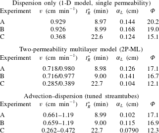
The fitted dispersivity (
 ${\it\alpha}_{L}$
) coefficients are provided in table 3 for each modelling scenario. The corresponding values of the objective function,
 ${\it\Phi}$
, and the model-predicted mean residence times,
 $t_{R}^{\ast }$
, are also given in the table. The agreement between the latter and the values obtained experimentally (
 $t_{R,exp}^{\ast }$
, reported in table 2) is very good irrespectively of the model used (2–3 %rel. deviation). This observation is well aligned with the common perception that the first temporal moment of the RTD function is not affected by the heterogeneity of the porous medium (Fogler Reference Fogler1999). We also note that within each modelling scenario, the value of the dispersivity is not constant, despite the latter represents a characteristic property (i.e. length scale) of the porous medium and should therefore be independent of the flow rate. This discrepancy (
 $\pm 0.02$
cm) is consistently found within each set of simulations and among repeated experiments (A–B), thus suggesting an experimental rather than modelling uncertainty. In the following, average values are therefore considered as being representative of each scenario, namely
 ${\it\alpha}_{L}=0.15\pm 0.02$
cm (1-D model),
 ${\it\alpha}_{L}=0.12\pm 0.02$
cm (‘2P-ML’) and
 ${\it\alpha}_{L}=0.10\pm 0.02$
cm (‘tuned streamtubes’ model). As expected, a larger dispersivity is found with the 1-D model as compared to both the ‘2P-ML’ and ‘tuned streamtubes’ models, because the former has to lump into one parameter the contributions from subcore-scale heterogeneities that are separately accounted for in the other two models through layers (or streamtubes) of different permeability.
Results from the modelling scenarios considered in this study that use three different maps to represent permeability heterogeneity (see § 3.2). The following properties are given: interstitial (pore) velocity (
 $v$
), mean residence time (
 $t_{R}^{\ast }$
), dispersivity (
 ${\it\alpha}_{L}$
, fitted) and sum of squared residuals (
 ${\it\Phi}$
).

4.2 Dynamic multidimensional imaging of tracer transport
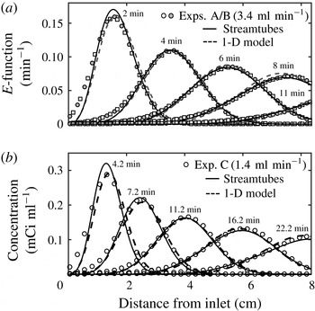
Figure 6 shows the slice-averaged activity profiles along the length of the core plotted at five distinct times for all pulse-tracer tests (A and B in (a) and C in (b)). These data have been obtained from the reconstructed PET scans by combining the measured voxel activity values,
 $A_{0j}^{PET}(t_{i})$
. Again, experimental data are represented with symbols, while the lines are predictions from the homogeneous (1-D, dashed lines) and the ‘tuned streamtubes’ model (solid lines). For tests A and B (
 $q=3.42~\text{ml}~\text{min}^{-1}$
, figure 6
a), the results are shown in terms of the function
 $E(t)$
, and demonstrate excellent repeatability. A very good agreement is also observed between experiment and model results, with the ‘tuned streamtubes’ (solid lines) approach providing a slightly better match than the simpler 1-D model (dashed lines). Note that the models are used here in a predictive mode, since only the effluent detectors’ data (shown in figures 4 and 5) have been used for fitting purposes. This not only confirms the ability of the ‘tuned streamtubes’ approach to describe tracer transport within the core sample, but also the suitability of an imaging technique, such as PET, to provide precise quantitative information of the tracer activity within an opaque porous medium both spatially and dynamically.
Slice-averaged tracer activity profiles measured from PET data plotted along the longitudinal axis of the sample at various times for experiments carried out at
 $q=3.42~\text{ml}~\text{min}^{-1}$
((a), experiments A, shown with circles, and B, shown with squares) and at
 $q=1.36~\text{ml}~\text{min}^{-1}$
(experiment C, (b)). The data in (a) are normalised by the total activity injected and are represented in terms of the RTD function,
 $E(t)$
. Symbols represent experimental data and lines are simulation results obtained upon applying the homogeneous (1-D, dashed line) or the ‘tuned streamtubes’ model (solid line).

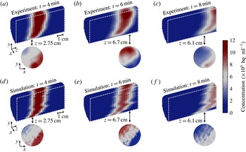
3-D PET reconstructions of the tracer activity,
 $A_{0j}^{PET}(t_{i})$
, in the rock sample during test A are shown in figure 7(a–c) at three different times (4, 6 and 8 min). These are presented in the form of longitudinal cross-sections to better elucidate the characteristic features of the tracer plume as it moves through the rock. As expected, the spreading of the tracer increases with distance travelled and, accordingly, its average concentration decreases, as confirmed by the gradual discolouration of the mixing zone. Moreover, the latter does not grow symmetrically, but it is characterised by a pronounced lag in the lower half of the sample. As shown in figure 7(d–f), this phenomenon is nicely reproduced upon application of the ‘tuned streamtubes’ model and can therefore be traced back to subcore-scale permeability heterogeneity. As anticipated earlier, the fine-textured layers that characterise the lower half of the sample (see figure 1) create an advective distortion in the spreading of the tracer on top of the expected hydrodynamic (‘Fickian’) dispersion. Notably, the streamtube model tends to enhance the former effect, thus resulting in profiles that are somewhat sharper (i.e. follow a zigzag pattern) than the smoother PET image frames. We believe that the main reason for this is that mass transfer across the tubes is neglected in the model. The latter, however, captures quite nicely the strong concentration gradients that are readily visible in the experimental two-dimensional (2-D) transect maps (
 $x$
–
 $y$
plane). This further suggests that the contribution of transverse dispersion to solute transport over the scale of this experiment is still very limited (e.g. to a length that is of the order of the size of an imaged voxel) and supports the assumption of a streamtube approach with negligible cross-flow.
Multidimensional maps of the tracer concentration within the rock sample at different times (
 $t=4$
, 6 and 8 min) for the experiment at
 $q=3.43~\text{ml}~\text{min}^{-1}$
(experiment A). Experimental data ((a–c), as obtained from the PET scanner) are compared to simulation results from the ‘tuned streamtubes’ model (d–f). Two-dimensional reconstructions of a single slice are also shown at selected positions along the longitudinal axis of the rock core (2.75, 6.7 and 6.1 cm). Each image has been reconstructed using a voxel size of (
 $2\times 2\times 3$
) mm3 and represents a 1-minute time frame.

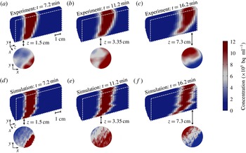
Figure 8 presents a similar multidimensional data set for test C. The agreement at any point in time and space between experimental observations and model predictions is striking. The similarity with the results shown in figure 7 confirm the reproducibility of the experiment technique and the importance of the characteristic internal structure of the sample in affecting the dynamic spreading of the tracer. Despite the lower flow rate, the concentration gradients in the direction perpendicular to flow are still very pronounced and support the conclusion of limited transverse dispersivity under these experimental conditions. We have additionally evaluated this assumption by computing from the decay-corrected PET images the total activity in each streamtube at different times. For each streamtube and over the time frame prior to significant breakthrough, cumulative changes were less than 10 %. This confirms that under the conditions of the experiments and for this specific sample cross-flow is very limited.
Multidimensional maps of the tracer concentration within the rock sample at different times (
 $t=7.2$
, 11.2 and 16.2 min) for the experiment at
 $q=1.36~\text{ml}~\text{min}^{-1}$
(experiment C). Experimental data ((a–c), as obtained from the PET scanner) are compared to simulation results from the ‘tuned streamtubes’ model (d–f). Two-dimensional reconstructions of a single slice are also shown at selected positions along the longitudinal axis of the rock core (1.5, 3.35 and 7.3 cm). Each image has been reconstructed using a voxel size of (
 $2\times 2\times 3$
) mm3 and represents a 1-minute time frame.

5 Discussion
Geological porous media can be regarded as hierarchical systems, since their heterogeneity ‘involves many different patterns of variability at a wide range of length-scales’ (Ringrose et al. Reference Ringrose, Sorbie, Corbett and Jensen1993). The practical implication of this situation is that the interpretation of a tracer BTC measured during a laboratory core flood can be as difficult as of those obtained at observation wells during field trials. In both cases, predicting the tracer production history requires a proper understanding of the system’s heterogeneities and of their effects on the dispersion process. Dispersivities obtained at the laboratory scale are often sample specific due to the presence of macroscopic (mm–cm) heterogeneities in reservoir cores (Walsh & Withjack Reference Walsh and Withjack1994) and are therefore not applicable to larger observational scales. In this context, the ability to decouple subcore scale heterogeneity effects from those of (true) hydrodynamic dispersion may lead to the estimation of dispersion coefficients that are representative of a rock type and better suited for up-scaling and extrapolating to longer transport distances. This approach was followed in this study, where we have applied [11C]PET for the dynamic imaging of miscible displacements in a Berea sandstone core. While the use of this technique to image flows in porous media has been reported previously (Khalili et al. Reference Khalili, Basu and Pietrzyk1998; Gründig et al. Reference Gründig, Richter, Seese and Sabri2007; Boutchko et al. Reference Boutchko, Rayz, Vandehey, O’Neil, Budinger, Nico, Druhan, Saloner, Gullberg and Moses2012; Fernø et al. Reference Fernø, Gauteplass, Hauge, Abell, Adamsen and Graue2015), the novelty of this work is its application to the study of hydrodynamic dispersion in rocks. The strength of the analysis lies in the approach that contains a significant deterministic component, because an independently measured 3-D permeability map of the sample is used to identify convective pathways and to build a streamtube model. While the spatial arrangement of the streamtubes in the model is known a priori and not allowed to change, the distribution of permeability values is slightly stretched, so as to match the measured effluent tracer curve. Once calibrated, the model uses the dispersivity as the sole fitting parameter and nicely reproduces the temporal and spatial evolution of the entire tracer plume imaged by PET.
We note that the use of a streamtube formulation to describe transport in our experiments assumes that Fickian behaviour holds at the voxel scale (
 ${\sim}$
10 mm3, corresponding to approximately 4500 grains). This is in agreement with previous theoretical observations on Berea sandstone (Bijeljic & Blunt Reference Bijeljic and Blunt2006), which suggest that for
 $Pe\approx 100$
asymptotic (i.e. Fickian) regime is attained at this scale after the solute has traversed
 ${\sim}$
1000 pores. While it admittedly represents an approximation, the use of streamtubes in our study is further justified in light of the particular geometry of the sample and the characteristics of the flow field. As discussed in the following, the coupling of PET with core-flooding experiments is very valuable, if not necessary, because conventional macroscopic observations (e.g. a BTC) are interpreted in the light of microscopic (i.e. subcore-scale) observations of dispersion processes that take place within the system itself. Even though a limit exists on the size of a laboratory sample, we argue that this ability to verify predictions across a range of scales has a value that goes beyond the absolute size of the system. In this context, the application of PET to other porous (and more heterogeneous) systems represents an opportunity to evaluate modelling approaches that are different (and more sophisticated) than the one proposed here, such as the ‘hybrid’ CTRW formulation (Berkowitz et al.
Reference Berkowitz, Cortis, Dentz and Scher2006), which combines deterministic and stochastic treatments of large- and small-scale heterogeneities, respectively.
5.1 Comparison with literature data
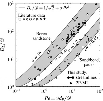
A
 $D_{L}/\mathscr{D}$
versus
 $Pe$
diagram is shown in figure 9 that compares the results from this study with data and correlations reported in the literature. The latter take the form of a power law
 $D_{L}/\mathscr{D}=1/\sqrt{2}+{\it\sigma}Pe^{{\it\delta}}$
(Sahimi et al.
Reference Sahimi, Hughes, Scriven and Davis1986), where
 ${\it\delta}\approx 1{-}1.2$
for measurements in bead/sand packs and (homogeneous) sandstones (Gist et al.
Reference Gist, Thompson, Katz and Higgins1990; Bijeljic & Blunt Reference Bijeljic and Blunt2006), while
 ${\it\sigma}$
is a parameter that describes the inhomogeneity of the medium and varies in the range
 ${\it\sigma}=0.5{-}28$
for experiments with unconsolidated and consolidated systems (Perkins & Johnston Reference Perkins and Johnston1963). Estimates based on this correlation are plotted in the figure for
 ${\it\delta}=1.2$
and four different values of the inhomogeneity factor, i.e.
 ${\it\sigma}=0.45,1.2,3.25,12$
. These outline two distinct regions, which are almost an order of magnitude apart, and include experimental results on sand/bead packs (plus and cross symbols) and on Berea sandstone cores (empty and filled symbols), respectively. While such discrepancy can be explained by the very different tortuosity that characterises the pore space of a consolidated and an unconsolidated porous medium, the reconciliation of the results obtained with the same rock type (i.e. Berea sandstone) is not as straightforward. For the flow regime
 $Pe=2{-}20$
, dispersion coefficients vary by approximately a factor of three for experiments carried out at a given
 $Pe$
. While some studies (Hulin & Plona Reference Hulin and Plona1989; Gist et al.
Reference Gist, Thompson, Katz and Higgins1990) report measured dispersivity values for Berea sandstone that are just above those obtained in this work, others have reported significantly larger values (e.g.
 $0.2{-}0.5$
cm) (Brigham et al.
Reference Brigham, Reed and Dew1961; Perkins & Johnston Reference Perkins and Johnston1963; Baker Reference Baker1977; Walsh & Withjack Reference Walsh and Withjack1994). We argue that such discrepancy is a direct manifestation of subcore-scale heterogeneities of rock samples and, specifically, of their spatial distribution and correlation length that may vary from sample to sample even when the same rock type is considered. It is therefore not surprising that both Fickian (Baker Reference Baker1977; Hulin & Plona Reference Hulin and Plona1989; Gist et al.
Reference Gist, Thompson, Katz and Higgins1990) and non-Fickian (Grattoni et al.
Reference Grattoni, Rosen, Chertcoff and Bidner1987; Walsh & Withjack Reference Walsh and Withjack1994; Cortis & Berkowitz Reference Cortis and Berkowitz2005) treatments of dispersion are reported in the literature for experiments carried out on Berea sandstone samples with a length of 10 cm and above.
Dispersion data plotted as a reduced longitudinal dispersion coefficient (
 $D_{L}/\mathscr{D}$
) as a function of the Péclet number,
 $Pe=vd_{P}/\mathscr{D}$
, where
 $\mathscr{D}$
is the molecular diffusion coefficient,
 $v$
is the interstitial (pore) fluid velocity and
 $d_{P}$
is the average particle (or grain) diameter. The solid lines are obtained from a common correlation found in the literature (Sahimi et al.
Reference Sahimi, Hughes, Scriven and Davis1986), i.e.
 $D_{L}/\mathscr{D}=1/\sqrt{2}+{\it\sigma}Pe^{{\it\delta}}$
, with
 ${\it\delta}=1.2$
and
 ${\it\sigma}=0.45,1.2,3.25,16$
. Literature data are represented by the symbols and include measurements on sand/bead packs, i.e. (
 $+$
) Dullien (Reference Dullien1992) and (
 $\times$
) Perkins & Johnston (Reference Perkins and Johnston1963), as well as those on Berea sandstone samples, i.e. (▫) Brigham et al. (Reference Brigham, Reed and Dew1961), (▹) Scheidegger (Reference Scheidegger1974) (after Cortis & Berkowitz (Reference Cortis and Berkowitz2005)), (▿) Baker (Reference Baker1977), (▵) Hulin & Plona (Reference Hulin and Plona1989), (○) Gist et al. (Reference Gist, Thompson, Katz and Higgins1990) and (♢) Honari et al. (Reference Honari, Bijeljic, Johns and May2015). Results from this study are given by the black-filled symbols, as obtained from the ‘tuned streamtubes’ (●) and ‘2P-ML’ (▴) models and by assuming
 $\mathscr{D}=1\times 10-5~\text{cm}^{2}~\text{s}^{-1}$
and
 $d_{P}=150~{\rm\mu}$
m.

We have shown in this study that non-Fickian behaviour in Berea sandstone can be caused by small yet significant permeability contrast at the subcore scale. This effect was captured by discretising the sample into an ensemble of streamtubes with distinct (and independently measured) permeability values, and by solving the ADE for each of them using the same dispersivity value,
 ${\it\alpha}_{L}$
. The latter has a value (
 ${\it\alpha}_{L}=0.10\pm 0.02$
cm) that is somewhat lower than those reported in earlier studies; we suggest that this is because it solely represents ‘Fickian’ (microscopic) dispersion. In other words, the obtained dispersivity is characteristic of a homogeneous medium and is therefore not sample specific. We note that, in the present study, the number of dispersion coefficients obtained at a given average flow rate corresponds to the number of layers (or streamtubes) used in the underlying permeability map, the dispersivity
 ${\it\alpha}_{L}$
taking a constant value, i.e.
 $D_{L}={\it\alpha}_{L}v$
. Accordingly, two points per experiment are shown for the ‘2P-ML’ model, while the results of the ‘tuned streamtubes’ model are plotted in the figure as pairs of values connected by solid lines that represents 431 dispersion coefficients (i.e. streamtubes) per average flow rate. It follows that for the new data set produced in this work (
 $6<Pe<30$
) the proportionality
 $D_{L}\propto Pe$
applies not only at the core scale for experiments carried out at different average flow rates, but also at the subcore scale, because of fluid velocity variations caused by permeability heterogeneity.
5.2 The importance of in-situ imaging for heterogeneous porous media
One of the features that distinguishes a laboratory rock sample from a field-scale setting is that the internal distribution of key transport parameters can be obtained with high precision and resolution thanks to the utilisation of non-invasive tomographic methods. This further implies that such systems are amenable to a deterministic rather than stochastic representation of transport. The latter has been shown to be very effective in the context of subsurface hydrology, where transport parameters (e.g. permeability) are typically mapped into a probabilistic framework, their exact distribution being typically poorly known (Steefel & Maher Reference Steefel and Maher2009). Moreover, such methods are commonly applied onto domains with sizes that are significantly larger (
 ${\sim}\!100\times$
) than the correlation length scale of the given transport parameter (Le Borgne et al.
Reference Le Borgne, Dentz, Bolster, Carrera, de Dreuzy and Davy2010; Meyer & Tchelepi Reference Meyer and Tchelepi2010). Laboratory rock core samples, on the other hand, tend to possess internal heterogeneities with correlation lengths that are similar in order as the size of the sample and cannot always be treated as ‘uniformly heterogeneous’ (Berkowitz et al.
Reference Berkowitz, Scher and Silliman2000). This is also the case for the 8.4 cm-long Berea sandstone core used in this study, where the observed permeability correlation length scale is of the order of a few cm. To account for this, the sample was mapped on a grid with about 12 000 cells of known porosity and permeability, and this information was used to build a streamtube model to solve the transport equation.
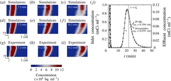
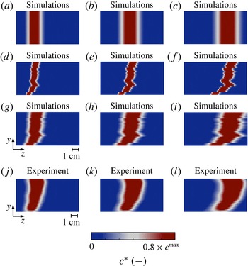
Among the various scenarios of permeability heterogeneity that have been investigated, the ‘2P-ML’ and the ‘tuned streamtubes’ models both provide a very good match of the tracer effluent profile, as shown on figure 10(j) for test C. An F-test confirms that the outcomes of the two models are, statistically speaking, not distinguishable (
 $F_{43,42}=0.7<F_{crit}=4,p=0.4$
at a 5 % significance level). This result is not very surprising, because the selection of the values and relative fractions of the pair of permeabilities used in the ‘2P-ML’ model was informed, i.e. it was based on the permeability distribution of the ‘tuned streamtubes’ model (see figure 1). Two-dimensional reconstructions of the tracer plume at different times are additionally shown in figure 10 to further compare experimental results with predictions from both models. It can be seen that the ‘2P-ML’ model (a–c) leads to an excessive smearing of the tracer plume in the lower half of the sample, as compared to the predictions from the ‘tuned streamtubes’ model (d–f), which resemble more closely to the experimental data (g–i). This effect is most likely caused by the contrasting permeability strikes that resulted from an oversimplification of the true permeability field of the sample. This result highlights once more the necessity of applying a non-invasive imaging tool, such as PET, to validate predictions from models that have been calibrated on a (macroscopic) BTC. We anticipate that the ability to correctly measure solute concentrations with such level of detail will disclose significant opportunities for PET to advance our understanding of more complex flows, such as those that involve chemical reactions, as the latter strongly depend on patterns of local mixing (Le Borgne et al.
Reference Le Borgne, Dentz, Bolster, Carrera, de Dreuzy and Davy2010).
The benefits of in-situ imaging: a comparison between 2-D reconstructions of the time evolution of the tracer plume as predicted from two different models that both yield an excellent fit of the measured effluent concentration profile (j), namely the ‘tuned streamtubes’ (
 ${\it\alpha}_{L}=0.079$
cm) (d–f) and the ‘2P-ML’ model (
 ${\it\alpha}_{L}=0.104$
cm) (a–c). (g–i) Shows the corresponding experimental results for the experiment at
 $q=1.36~\text{ml}~\text{min}^{-1}$
experiment C). Voxel size: (
 $2\times 3$
) mm2.

A visual appraisal of the distinct contributions of hydrodynamic dispersion and permeability heterogeneity to miscible displacements in rocks: simulation results representing the central cross-section along the longitudinal axis of the sample as obtained from three distinct scenarios, namely ‘dispersion only’ (i.e. homogeneous core with
 ${\it\alpha}_{L}=0.079$
cm) (a–c), ‘advection only’ (i.e. ‘tuned streamtubes’ with
 $0.1\times {\it\alpha}_{L}$
) (d–f) and ‘advection–dispersion’ (i.e. ‘tuned streamtubes’ with
 ${\it\alpha}_{L}=0.079$
cm) (g–i). The last row (j–l) shows the corresponding experimental results at different times (
 $t_{1}=7.2$
min,
 $t_{2}=11.2$
min and
 $t_{3}=16.2$
min) for the experiment at
 $q=1.36~\text{ml}~\text{min}^{-1}$
(experiment C). Voxel size: (
 $2\times 2\times 0.5$
) mm3. The colour scale ranges from zero to a value that is 80 % of the maximum concentration observed in the given map.

Dynamic spreading of the tracer plume plotted as a function of the square root of the distance travelled. The longitudinal distortion,
 $|L_{m}|$
, is defined as the difference between the position of the centre of mass of the tracer’s plume and the position at which the tracer concentration is dropped to a value that is 20 % of the maximum concentration observed within the plume at a specific time. The symbols (●) represent simulation results from the ‘dispersion only’ scenario (i.e. homogeneous system with
 ${\it\alpha}_{L}=0.079$
cm) at three different times (7.2, 11.2 and 16.2 min). The grey-shaded histograms are results from the ‘advection only’ scenario (i.e. ‘tuned streamtubes’ with
 $0.1\times {\it\alpha}_{L}$
), while the white-faceted histograms represent the ‘advection–dispersion’ scenario (i.e. ‘tuned streamtubes’ with
 ${\it\alpha}_{L}=0.079$
cm). The PET measurements are shown with solid lines, which have been obtained by fitting a kernel probability distribution function to the experimental histogram (MATLAB function ‘fitdist’ with a bandwidth value of 2).

5.3 Permeability heterogeneity and hydrodynamic dispersion
Two additional simulation scenarios have been considered to assess the individual contributions of advection (i.e. permeability heterogeneity) and dispersion to the spatial evolution the tracer plume as it moves through the rock sample. These include (i) a simulation that uses the optimum dispersivity value obtained from the fitting of the experimental data (‘tuned streamtubes’ model,
 ${\it\alpha}_{L}=0.079$
cm), but neglects permeability heterogeneity (‘dispersion only’), and (ii) a simulation that accounts for permeability heterogeneity, but neglects dispersion (‘advection only’). The simulation results are presented in figure 11 as still frames of the central longitudinal cross-section of the core sample. These are compared to a model prediction that accounts for both effects (‘advection–dispersion’) and to the results from PET imaging. It can be seen that the effects of permeability heterogeneity (figure 11
d–f) are indeed significant and lead to a distortion of the tracer plume in the direction of flow that is similar in order as the spreading caused by hydrodynamic dispersion alone (a–c). Notably, only when the two mechanisms are combined in the model a satisfactory match is obtained with the experimental observation (g–i and j–l). To quantitatively support this conclusion, we have computed the distance between the centre of mass of the tracer plume and its outer limits (identified from the position at which the concentration has dropped to 20 % of its maximum value) at different times. We refer to this distance as the ‘longitudinal distortion’,
 $L_{m}$
(Dullien Reference Dullien1992). The results from this exercise are shown in figure 12, where
 $|L_{m}|$
is plotted as a function of the square root of the mean distance travelled for the three scenarios. In the figure, the black-filled circles represent the ‘dispersion only’ scenario; here, only one value of
 $L_{m}$
is needed to describe the spreading of the tracer plume at each given time (because ‘Fickian’ dispersion is ubiquitous) and the expected linear growth is observed (
 $L_{m}^{\text{1D}}\propto \sqrt{t}$
). Results obtained from the models accounting for permeability heterogeneity are shown in histogram form to represent the distribution of travel times along each streamtube (
 $431\times 2=862$
values per time step). As expected, the contribution of the advection component (grey-shaded bins) to longitudinal dispersion is relatively small at short distances and increases with distance travelled. Notably, for a significant number of streamtubes the effects of permeability heterogeneity alone become even stronger than those of hydrodynamic dispersion, as shown by the bins found above the dashed line in the figure. Accordingly, when the two mechanisms are combined in the advection–dispersion scenario (white-faceted bins) the width of the distribution increases significantly and the plume extends well beyond the limits set by the homogeneous ‘Fickian’ model. Again, good quantitative agreement is observed between the predictions from the advection–dispersion scenario and the PET measurements (shown by the solid line). This result is important, because it highlights that the effects of subcore-scale permeability heterogeneity in rock samples can be as significant as those of hydrodynamic dispersion and, therefore, that the former should not be neglected to predict solute transport in these systems. While this has been demonstrated in this study for a Berea sandstone core, we argue that this conclusion is more general and applies to other rock types (e.g. carbonates, Bijeljic et al.
Reference Bijeljic, Mostaghimi and Blunt2011) that are likely to be more heterogeneous.
6 Concluding remarks
We have successfully applied [11C]PET and X-ray CT to image and quantify solute spreading and mixing in Berea sandstone during pulse-tracer tests in the
 $Pe$
regime 6–40. Although Berea sandstone is commonly considered as the archetype of a homogeneous rock, an analysis of the literature shows that approaches used to describe transport in this system are opposite, thus including both Fickian and non-Fickian formalisms. We provide direct experimental evidence in this study that non-Fickian behaviour in Berea sandstone is caused by small yet significant permeability contrast at the subcore (
 ${\sim}$
mm) scale. We also report on the unprecedented benefits that arise from the combined application of the two imaging techniques for studying transport in heterogeneous porous systems. While X-ray CT is a well-established (and necessary) characterisation tool in the context of reservoir core analyses, PET allows visualising the spatial evolution of the full tracer plume with a temporal resolution not readily accessible by the former.
An experimental protocol is presented that integrates (i) conventional macroscopic observations (i.e. a tracer effluent curve), (ii) subcore (
 ${\sim}$
10 mm3) scale quantification of heterogeneities (e.g. porosity and permeability) and (iii) direct dynamic observation of the subcore-scale displacement process. We observe that solute spreading in the rock sample is affected by significant longitudinal macrodispersion effects, together with negligible transverse mixing at the subcore scale. Accordingly, a streamtube model is applied to describe solute transport that is based on the 1-D advection–dispersion equation and that assumes instantaneous intrastreamtube lateral mixing and zero interstreamtube mixing.
Our approach represents a departure from previous studies, because the streamtubes’ spatial arrangement and travel times are known from an independently measured subcore-scale permeability map of the rock sample and require only a minor adjustment against a measured tracer breakthrough curve. As such, the model is applied in a semideterministic fashion and uses the intrastreamtube longitudinal dispersivity as the sole fitting parameter. Most importantly, the model reproduces accurately the spatial and temporal evolution of the full tracer plume for each pulse-tracer test. The ability to decouple subcore-scale permeability heterogeneity effects from those of local dispersion in Berea sandstone leads to the estimation of a dispersivity that is not sample specific and that therefore possesses a true predictive value. We argue that effects of macrodispersive spreading are likely to overcome those of local dispersion for rocks that are more heterogeneous than Berea sandstone. In this context, the use PET in combination with X-ray CT provides significant opportunities to advance our understanding of miscible displacements in consolidated porous media, thus including those involving additional phenomena, such as adsorption, chemical reactions and capillary effects.
Acknowledgements
The authors would like to thank J. Jones (Medical Imaging Systems, Siemens, United States) and C. Michel (Molecular Imaging Division, Siemens, United States) for contributions made in the reconstruction of the PET images.