1 Introduction
Flow around bluff bodies has attracted extensive research for more than 200 years, especially since the discovery of Kármán vortex streets. A vast amount of research has been focused on flow around stationary circular and rectangular/square cylinders; see Williamson (Reference Williamson1996), Zdravkovich (Reference Zdravkovich1997), Matsumoto (Reference Matsumoto1999), Thompson, Leweke & Williamson (Reference Thompson, Leweke and Williamson2001), Mills, Sheridan & Hourigan (Reference Mills, Sheridan and Hourigan2003) among others. In addition to the important governing parameter, the Reynolds number
 $Re$
, special attention was also usually paid to the Strouhal number
 $St$
, drag coefficient
 $C_{D}$
and fluctuating lift coefficient
 $C_{L}^{\prime }$
, which are closely associated with the vortex shedding dynamics.
Roshko (Reference Roshko1955) discovered for the first time that, as
 $C_{D}$
increases,
 $St$
decreases and this relation is particularly pronounced after the boundary layer transition (hereafter the transition). He also found that the vortex-shedding frequency is related to the wake width (distance between the free streamlines separating the wake and the distorted potential outer flow, denoted
 $D_{w}$
), instead of the physical width of the bluff body (
 $D$
) and proposed a wake Strouhal number
 $St^{R}$
(also called the universal Strouhal number), viz.
 $$\begin{eqnarray}St^{R}=\frac{f_{s}D_{w}}{U_{s}},\end{eqnarray}$$
where
 $f_{s}$
is the vortex-shedding frequency,
 $U_{s}$
is the free-stream velocity outside the boundary layer at the separation point, which is also the velocity at which the shed vortices are swept downstream. Gerrard (Reference Gerrard1966) proposed another Strouhal number, viz.
 $$\begin{eqnarray}St^{G}=\frac{f_{w}l_{f}}{U_{\infty }},\end{eqnarray}$$
where
 $f_{w}$
is the fundamental wake frequency,
 $l_{f}$
is the vortex formation length and
 $U_{\infty }$
is the free-stream velocity. He also discussed the importance of the diffusion length, which is the transverse thickness of the shear layer at the end of the vortex formation region. Williamson (Reference Williamson1988) proposed a relation between the universal
 $St$
and
 $Re$
for laminar vortex shedding from a circular cylinder and Ponta (Reference Ponta2006) further discussed the influence of the shear layer thickness on this relation. Norberg (Reference Norberg2003) summarised previous measurement methods and conducted new measurements of
 $C_{L}^{\prime }$
. He suggested a mathematical relation between
 $C_{L}^{\prime }$
and
 $Re$
, and pointed out a fundamental change in the mode of vortex shedding (high- and low-quality mode of turbulent shedding, respectively) before the subcritical regime (
 $5.0\times 10^{3}\lesssim Re\lesssim 8.0\times 10^{3}$
), where
 $Re\equiv U_{\infty }D/\unicode[STIX]{x1D708}$
(
 $\unicode[STIX]{x1D708}$
is the kinematic viscosity).
Since the work of Roshko (Reference Roshko1955), a number of researchers have tried to establish more accurate or robust relations between
 $C_{D}$
and
 $St$
. For example, Hoerner (Reference Hoerner1965) proposed an empirical relation
 $0.21=C_{D}^{0.75}St$
applicable for
 $Re>10^{3}$
and for two-dimensional bodies like flat plates, aerofoils and cylinders. Bearman (Reference Bearman1967) showed that the product
 $C_{D}St$
only depends on
 $\sqrt{1-(C_{p})_{b}}$
, where
 $(C_{p})_{b}$
is the base pressure coefficient. Yeung (Reference Yeung2010) also established a relation between
 $C_{D}St$
and
 $\sqrt{1-(C_{p})_{b}}$
from data of an inclined flat plate, a rectangular section, a circular cylinder and a
 $90^{\circ }$
wedge. Based on the conservation of mass, momentum and energy, Ahlborn, Seto & Noack (Reference Ahlborn, Seto and Noack2002) proposed a phenomenological model for the vortex-shedding process behind cylindrical bodies. They obtained a relation between
 $St$
,
 $Re$
,
 $C_{D}$
and geometric wake parameters through the definition of a universal
 $St$
based on the size of an individual shed vortex. Alam & Zhou (Reference Alam and Zhou2008) conducted a theoretical analysis based on the conservation of the averaged kinetic energy given no energy exchange between the bluff body and its support. They showed on the basis of experimental data reported in the literature, as well as their own data, that the product
 $C_{D}St$
is approximately a constant, which is almost independent of the shape of a bluff body, its angle of attack and
 $Re$
.
Polygonal cross-section slender cylinders with a finite number of sides
 $N\geqslant 3$
are commonly seen in engineering problems, e.g. skyscrapers, floating tunnels, prototype supporting frames in wind tunnel tests. Similar to a circular cylinder (
 $N=\infty$
), flow around a polygonal cylinder is characterised by the instability of the boundary layer, laminar–turbulent transition, separation, unsteady vortex shedding etc. Unfortunately, in contrast to the vast number of papers published on the circular cylinder wake, there has been little attention in the literature paid to the fluid dynamics of the polygonal cylinder with
 $N>4$
in cross-flow, and the relative data are scarce. Whenever an engineering problem related to the polygonal cylinder is encountered, a usual approach is to use the data of circular or square cylinders, which are well documented, as approximations. In some circumstances, however, such an approach can be very risky since the fluid dynamics associated with a polygonal cylinder can be significantly different from that involving a circular or a square cylinder, even under the same flow conditions, as will be demonstrated in this work.
Among the relatively limited number of research papers on the polygonal cylinder wake, Tian & Li (Reference Tian and Li2007) investigated a polygonal cylinder of
 $N=24$
(N24 in abbreviation, and similar for other polygons hereafter) in a low-speed wind tunnel to seek a low drag solution for their prototype supporting frames. They found a much lower critical Reynolds number (
 ${\approx}1.0\times 10^{5}$
) and 40 % drag deduction with a low level fluctuation compared to a circular cylinder case under similar flow conditions. Bosch & Guterres (Reference Bosch and Guterres2001) tested a N8 tapered cylinder in their wind tunnel at
 $Re\approx 3.0\times 10^{3}\sim 2.0\times 10^{4}$
and found that the drag for the face orientation is lower than that for the corner orientation, and the degree of taper has a significant effect on the aerodynamic performance. Skews (Reference Skews1991, Reference Skews1998) found that the polygonal cylinder, whose ends were not fixed, with
 $N<8$
may undergo a spontaneous rotation, producing a larger lift than a circular cylinder at a similar rotation condition. Srigrarom & Koh (Reference Srigrarom and Koh2008) conducted flow visualisation and phase-locked particle image velocimetry (PIV) measurements on an equilateral triangular cylinder and found that, at certain uniform incoming flow velocities, the cylinder can oscillate persistently after an initial perturbation. Deniz & Staubli (Reference Deniz and Staubli1997) performed force and flow visualisation measurements for transversely oscillating rectangular and octagonal profiles and found that the mechanisms leading to energy transfer from the fluid to the structures are associated with the phase shift of the fluctuating lift forces with respect to the body oscillation.
There have been attempts to simulate numerically the flow around a polygonal cylinder. Tian & Wu (Reference Tian and Wu2009) calculated the flow field around two-dimensional polygonal cylinders at the corner orientation condition for even values of
 $N$
and
 $Re<200$
. They found through conformal mapping that, for the inviscid flow cases, the global pressure difference along the surface is inversely proportional to a value of
 $N$
that is sufficiently large. For the viscous flow cases, however, they derived the relation between the first critical
 $Re$
and
 $N$
, and found that this
 $Re$
decreases as
 $N$
increases. Khaledi & Andersson (Reference Khaledi and Andersson2011) investigated numerically flow after a hexagonal cylinder for both corner- and face-oriented cases up to
 $Re=10^{3}$
and found that the vortex-shedding frequency is higher in the latter case, which is opposite to the earlier findings for the square cylinders (e.g. Vickery Reference Vickery1966). The numerical works mentioned are inevitably limited to
 $Re$
lower than that typically seen in engineering applications.
To the best of the authors’ knowledge, there has been no systematic experimental investigation on the wake of a polygonal cylinder for
 $N\geqslant 5$
, especially for pentagonal and septilateral cylinders. This work aims to address this issue by measuring
 $C_{D}$
,
 $C_{L}^{\prime }$
and
 $St$
and determining their dependence on
 $N$
, along with the major flow characteristics, for different polygon orientations (corner or face).
2 Experimental details
Experiments were conducted in an open-loop low-speed wind tunnel, which has a square test section of
 $0.5~\text{m}\times 0.5~\text{m}\times 2~\text{m}$
. The wind speed is
 $2\sim 40~\text{m}~\text{s}^{-1}$
in the test section, and the turbulence intensity
 $\unicode[STIX]{x1D716}$
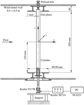
is no more than 0.5 % for the range of speeds we are presently concerned with. A schematic diagram of the side view of the section is shown in figure 1, where the coordinate system
 $(x,y,z)$
is defined. The tested model is installed vertically along the
 $z$
-axis. The lower end of the model is mounted with a three-component force measurement transducer Kistler 9317B, which is connected to a four-channel signal amplifier Kistler 5073A and a data collection A/D (analog/digital) board NI6221. The upper end is pin-supported on a pre-load bolt, which acts to eliminate the flow-induced cylinder vibration. Two circular-shaped end plates of Ø150 mm, typically
 $6\times$
the longitudinally projected width
 $D$
(see figure 2 for definition) of the test model, are attached near the two ends of the cylinder to eliminate the three-dimensional effects from the cylinder end and the possible influence from the wind tunnel walls. The gap between the end plates and the cylinder surface is 1 mm. The purpose of the end plate will be further elaborated at the end of this section.
Schematic of the experimental set-up.

The tested models include a flat plate (
 $N=2$
), the polygonal cylinders of
 $N=3{-}8$
, 12, 16 and a circular cylinder (
 $N=\infty$
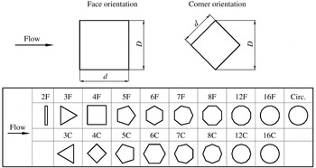
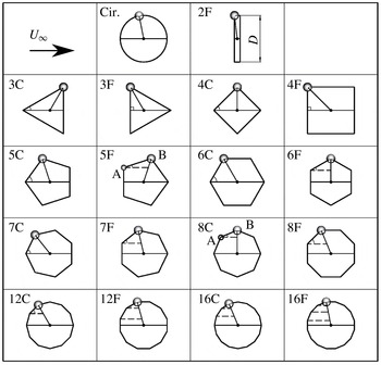
). Two principal orientations with respect to the incoming flow are examined for each of the polygonal cylinders, i.e. the face orientation, where one flat surface of the polygon faces normally to the incoming flow (denoted by NF), and the corner orientation, where the polygon is rotated so that one corner faces the incoming flow (denoted by NC), as shown in figure 2, where the orientation of the flat plate is also given. When placed in parallel with incoming flow, the flat plate is not considered as a bluff body and therefore is not tested. For most of the test cases,
 $D=25$
mm, resulting in a blockage ratio
 $\unicode[STIX]{x1D719}\approx 5\,\%$
. Larger
 $D$
, up to 50 mm, is also used for some cases to obtain the data of a larger
 $Re$
, which will be discussed later. All the cylinders are made from aluminium with a length
 $L=460$
mm (420 mm between the end plates) and an aspect ratio
 $L/D=16.8$
for
 $D=25$
mm.
Cross-sectional shapes, orientations (with respect to the incoming flow) and notations of the 18 tested polygonal cylinders (
 $2\leqslant N\leqslant 16$
) and the definition of the streamwise projected width
 $D$
. In notation/abbreviation NF and NC,
 $N$
is the polygon side number and F and C stand for orientations with a polygon flat surface and a corner, respectively, leading and facing normally to the incoming flow.

Load cells Kistler 9317B and Kistler 5073A are used to measure the time-averaged drag coefficient
 $C_{D}$
and the fluctuating root-mean-square lift coefficient
 $C_{L}^{\prime }$
. The resolution of the transducer is sufficiently high for our purpose (Alam & Zhou Reference Alam and Zhou2007). The force measurement signal is sampled at 5 kHz, which is approximately 12 times the highest
 $f_{s}$
from the cylinders. The sampling duration for each test is 5 s. The Strouhal number
 $St=f_{s}D/U_{\infty }$
is also extracted from the force signal. The agreement of the measured cylinder oscillation frequency and
 $f_{s}$
is confirmed by a simultaneous hot-film measurement at
 $2.5D$
downstream of the cylinders at the mid-span location (figure not shown).
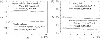
Figure 3 presents a comparison between the presently measured
 $C_{D}$
and
 $St$
for the circular cylinder and 4F cases and those reported in the literature. Evidently, for the examined
 $Re$
range,
 $C_{D}$
of the circular cylinder agrees well with Tropea, Yarin & Foss (Reference Tropea, Yarin and Foss2007), and so does that of 4F with White (Reference White2001). The maximum deviation is approximately 5 %. Agreement in
 $St$
is also quite good between the present and previously reported data; the departure is no more than 2 % over the entire
 $Re$
range examined.
Dependence of
 $C_{D}$
(a) and
 $St$
(b) on
 $Re$
for the case of 4F and the circular cylinder, as compared to the data available in the literature. Results are obtained from an average of seven repeated measurements.

The flow field is measured both qualitatively and quantitatively at a frame rate of 4 Hz by a LaVision PIV system, which consists of an Imager ProX camera with
 $2048\times 2048$
pixel CCD (charge coupled device) size and a low-speed duo-head Nd:YAG laser. The field of view (FOV) of the camera is typically
 $125~\text{mm}\times 125~\text{mm}$
. Flow is seeded by smoke generated from vegetable oil with a droplet size of approximately
 $1~\unicode[STIX]{x03BC}\text{m}$
in diameter. The smoke generator is located between six honeycomb meshes in the settling chamber of the wind tunnel, so that the smoke particles can be well mixed with air and form homogeneous smoke streaks. The PIV images are processed by DaVis 7.2 with final interrogation window (IW) size 32 pixel
 $\times$
32 pixel and 50 % overlap which gives a spatial resolution of 1.95 mm based on the IW size. For each test case, 100 velocity fields are acquired. Note that turbulence quantities are not of interest in this work. Smoke streak images are also used for flow visualisation after an appropriate increase of the laser power and the smoke particle density.
All experiments were conducted under room conditions. The
 $Re$
range is
 $1.0\times 10^{4}\sim 6.0\times 10^{4}$
. All the data presented in this paper for
 $Re\leqslant 6.0\times 10^{4}$
are from the cylinders of
 $D=25$
mm. Cylinders of
 $D=50$
mm are used for some cases in order to extend the
 $Re$
range to of the order of
 $10^{5}$
. The
 $Re$
for the PIV measurements are fixed at
 $1\times 10^{4}$
. Each testing case is measured more than three times to ensure repeatability.
West & Apelt (Reference West and Apelt1982) found that the effect of
 $\unicode[STIX]{x1D719}$
, if less than 6 %, is minor on
 $C_{D}$
and negligible on
 $St$
. They suggested that a correction is needed if
 $\unicode[STIX]{x1D719}>6\,\%$
. The correction factor is a function of
 $\unicode[STIX]{x1D719}$
and
 $C_{D}$
may decrease by 3 %–5 % after applying the correction. No correction is applied presently since
 $C_{D}$
and
 $St$
obtained from larger
 $D$
cylinders are found to be consistent with their counterparts from the cylinders of small
 $D$
.
It is worth pointing out that it is impossible to eliminate completely the three-dimensional end effects on the flow even if the end plates are installed and
 $L/D$
is kept large (Norberg Reference Norberg1994). Nevertheless, we have observed a considerable influence on the aerodynamic loading on the circular cylinder when the end plates are removed: the
 $C_{D}$
drops by 20 % and
 $St$
by 10 %, which is in agreement with previous reports by e.g. Cowdrey (Reference Cowdrey1962), Gerich & Echelmann (Reference Gerich and Echelmann1982) and Szepessy & Bearman (Reference Szepessy and Bearman1992). Norberg (Reference Norberg1994) also pointed out that for
 $1.0\times 10^{4}<Re<4.0\times 10^{4}$
,
 $L/D$
should be no-less than 25 to ensure good two-dimensionality. However, the agreement of the present results to the previous ones shown in figure 3 indicates that the present
 $L/D=16.8$
is acceptable.
3 Results
3.1 The effect of
 $Re$
on
$C_{D}$
and
$St$


The dependence of
 $C_{D}$
and
 $St$
on
 $Re$
has been well documented for the polygonal cylinders of
 $N\leqslant 4$
and
 $N=\infty$
. This work will be focused on the polygonal cylinders of
 $N>4$
, for which the information on
 $C_{D}$
and
 $St$
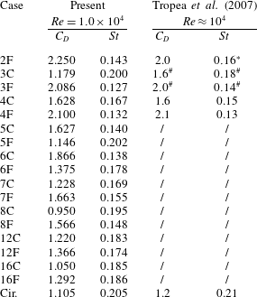
is scarce in the literature. Table 1 lists the presently measured
 $C_{D}$
and
 $St$
at
 $Re=1.0\times 10^{4}$
. The data for
 $N\leqslant 4$
and
 $N=\infty$
are also included for the purpose of comparison. There is in general a reasonable agreement between the present data and those in Tropea et al. (Reference Tropea, Yarin and Foss2007). There is a significant discrepancy in
 $C_{D}$
and
 $St$
for the case of 3C, marked by #. This is because the cross-sectional shape of the cylinder in Tropea et al. (Reference Tropea, Yarin and Foss2007) is a
 $90^{\circ }$
wedge, different from the present equilateral triangle. The present
 $St$
for 2F is lower than that in Tropea et al. (Reference Tropea, Yarin and Foss2007), marked by an asterisk, but is closer to that (0.13) reported in Blevins (Reference Blevins1990).
The present
 $C_{D}$
and
 $St$
values obtained at
 $Re=1.0\times 10^{4}$
. Also included are the reported data in Tropea et al. (Reference Tropea, Yarin and Foss2007).

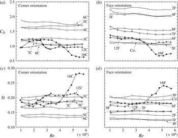
Figure 4 shows how
 $C_{D}$
and
 $St$
change as
 $Re$
varies from
 $1.0\times 10^{4}$
to
 $5.8\times 10^{4}$
, for all polygonal cylinders at both principal orientations, including the flat plate (2F) and the circular cylinder. The
 $C_{D}$
of the N12 and N16 cylinders declines rather rapidly from
 $Re\approx 3.0\times 10^{4}$
to
 $4.0\times 10^{4}$
and meanwhile the corresponding
 $St$
rises sharply. The observation points to a boundary transition from laminar to turbulent state. The effect of the transition on the changes of
 $C_{D}$
and
 $St$
can differ significantly when the cylinder changes its orientation. For example,
 $C_{D}$
decreases by 25 % and
 $St$
increases by 15 % from
 $Re\approx 2.4\times 10^{4}$
to
 $3.0\times 10^{4}$
for the 12C orientation, but the changes contract to 15 % and 5 %, respectively, for the 12F orientation. Furthermore, the
 $Re$
at which the transition starts to take place also varies from one orientation to the other. It can be inferred that the flow characteristics can be very different between the two orientations. On the other hand,
 $C_{D}$
and
 $St$
for
 $N\leqslant 8$
cylinders vary little, within
 $\pm 8\,\%$
and
 $\pm 4\,\%$
, respectively, over the entire
 $Re$
range, suggesting no change of the boundary layer state.
Dependence of
 $C_{D}$
and
 $St$
on
 $Re$
for both principal orientations. (a)
 $C_{D}$
for NC; (b)
 $C_{D}$
for NF; (c)
 $St$
for NC; (d)
 $St$
for NF; the cases for the flat plate and the circular cylinder are also included, denoted as 2F and Cir., respectively, in (b) and (d).

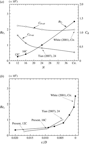
Figure 5(a) summarises the variation in the critical Reynolds number
 $Re_{c}$
, at which the boundary layer transition from laminar to turbulent state occurs, with increasing
 $N$
for the NC cases. The N24 case from Tian & Li (Reference Tian and Li2007) and the circular cylinder case (
 $N=\infty$
) from White (Reference White2001) are also included. The
 $Re_{c}$
is defined at the middle of the rapidly falling
 $C_{D}$
region in figure 4(a). The
 $C_{D}$
values before and after the transition, i.e.
 $C_{D\text{-}sub}$
and
 $C_{D\text{-}sup}$
, are also presented for each case. The NF cases are not shown since the transition effect on 12F is not very strong. Clearly, both
 $Re_{c}$
and
 $\unicode[STIX]{x0394}C_{D}=(C_{D\text{-}sub}-C_{D\text{-}sup})$
rise with increasing
 $N$
. The dependence of
 $Re_{c}$
on
 $N$
may be used to estimate
 $Re_{c}$
for the polygons that are not measured presently. For instance, the
 $Re_{c}$
of the 20C case is predicted to be about
 $7.0\times 10^{4}$
.
(a) Dependence of the critical Reynolds number
 $Re_{c}$
(●),
 $C_{D\text{-}sub}$
(○) and
 $C_{D\text{-}sup}$
on the polygon side number
 $N$
, for
 $N\geqslant 12$
for the corner orientation. (b) Dependence of
 $Re_{c}$
on the roughness height
 $\unicode[STIX]{x1D700}/D$
; ○: polygons, ▪: circular cylinders with roughness elements.

Given an adequately large
 $N$
, the corners of a polygonal cylinder may be considered to be wedge-shaped roughness elements evenly distributed on the surface of a circular cylinder with a radius
 $R_{i}$
. Denoting the distance between one corner and the polygon centroid as
 $R_{o}$
, the roughness height
 $\unicode[STIX]{x1D700}$
can be written as:
 $$\begin{eqnarray}\frac{\unicode[STIX]{x1D700}}{D}=\frac{R_{o}-R_{i}}{D}\approx \frac{1-\cos (\unicode[STIX]{x03C0}/N)}{2}.\end{eqnarray}$$
In an attempt to understand the positive correlation between
 $Re_{c}$
and
 $N$
shown in figure 5(a),
 $Re_{c}$
is plotted against
 $\unicode[STIX]{x1D700}/D$
in (b). One may recognise that the variation in
 $Re_{c}$
against
 $\unicode[STIX]{x1D700}/D$
for large
 $N$
polygonal cylinders agrees reasonably well both qualitatively and quantitatively with its counterpart for the rough-surfaced circular cylinders. It may be inferred that, given an adequately large
 $N$
,
 $Re_{c}$
of the polygonal cylinder may be estimated from that of the rough-surfaced circular cylinder, subjected to a small uncertainty. Güven, Farell & Patel (Reference Güven, Farell and Patel1980) observed that larger roughness elements on the surface of a circular cylinder gave rise to a thicker and more retarded boundary layer. As a result, the transition to turbulence occurred at lower
 $Re$
. As the roughness elements diminished in size, the drop in
 $C_{D}$
from subcritical to supercritical regime became more pronounced. The result shown in figure 5, i.e. increasing
 $Re_{c}$
and
 $\unicode[STIX]{x0394}C_{D}$
with larger
 $N$
or smaller
 $\unicode[STIX]{x1D700}/D$
, is fully consistent with their observation. The result further points to an analogy between polygonal cylinders of large
 $N$
and roughened circular cylinders.
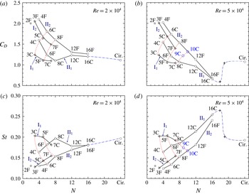
Dependence of
 $C_{D}$
(a,b) and
 $St$
(c,d) on the polygon side number
 $N$
for
 $Re<Re_{c}$
(a,c) and
 $Re>Re_{c}$
(b,d). The transition occurs at
 $N=12$
, 16. Data points 9C and 10C in (b) are two examples of the predicted results. The dash-dot lines denote the indicative trend for the polygons of large
 $N$
. The data points of 2F in (a) and (b) are from Tropea et al. (Reference Tropea, Yarin and Foss2007) and from Blevins (Reference Blevins1990) in (c) and (d). The two
 $+$
symbols in (b) and (d) indicate the turning points of the indicative trend lines from
 $N=16$
to the circular cylinder.

Note that figure 5(b) includes only the cases of
 $N\geqslant 12$
. For
 $N\leqslant 8$
, the corner number of the polygon is so low that
 $(R_{o}-R_{i})$
becomes relatively large compared to the characteristic dimension
 $R_{i}$
of the polygon and cannot be approximated as roughness elements any more. Therefore, the analogy between the polygon corners and roughness elements is no longer valid.
3.2 Dependence on
$N$
of
$C_{D}$
,
$St$
and
$C_{L}^{\prime }$


Figure 6 presents the dependence on
 $N$
of the measured
 $C_{D}$
and
 $St$
for both orientations of the polygons at
 $Re=2.0\times 10^{4}$
and
 $5.0\times 10^{4}$
, which correspond to the flow before and after the transition, respectively, of the N12 and N16 polygons. One may note that at small
 $N$
the
 $C_{D}$
or
 $St$
values differ greatly between the two orientations. However, this difference diminishes as
 $N$
becomes large, regardless of the orientation. While
 $C_{D}$
in general tends to decline with increasing
 $N$
,
 $St$
rises. There is another interesting observation, that is, the NF and NC data points (
 $C_{D}$
and
 $St$
) appear to form a distorted Cartesian mesh pattern, as highlighted by the solid and dashed lines. It is worthwhile conducting an analysis of the mesh pattern, which can be of practical importance, i.e. predicting
 $C_{D}$
and
 $St$
for the polygonal cylinders not measured presently. Four solid lines can be identified for each
 $Re$
, viz.
-
(i)
$\text{I}_{1}$
,
$N=2n+1$
; C oriented for odd
$n$
; F oriented for even
$n$
; -
(ii)
$\text{II}_{1}$
,
$N=2n$
; C oriented for even
$n$
; F oriented for odd
$n$
; -
(iii)
$\text{I}_{2}$
,
$N=2n+1$
; F oriented for odd
$n$
; C oriented for even
$n$
; -
(iv)
$\text{II}_{2}$
,
$N=2n$
; F oriented for even
$n$
; C oriented for odd
$n$
.


On each of the four solid lines, the F- and C-orientated data points are separated from each other, provided that the untested cases (e.g.
 $N=9,10$
), which can be estimated from the available data, are also included. The estimation of the untested cases will be explained below. There are actually more dashed lines than those marked in figure 6. For example, 2F–3F–4F can also form a dashed line. Unlike the solid lines, the data points along each of the dashed lines are of either uniformly
 $F$
or uniformly
 $C$
orientation. This particular pattern is essentially connected to the geometry of the polygons near the lateral maximum width points (the top and the bottom point) and the position of the flow separation point if the transition takes place (
 $N=12,16$
), which will be discussed in § 3.4.
The pattern shown in figure 6 can be used to predict approximately
 $C_{D}$
and
 $St$
for the cases that are not tested in the current experiment. For instance, based on the characteristics of the solid lines listed from item (i) to item (iv) above, it can be predicted from figure 6(b) that case 10C should be on the solid line
 $\text{I}_{2}$
and can be determined at the intersection of
 $\text{II}_{2}$
and
 $N=10$
. Connecting points 7C, 8C and 10C smoothly forms a new dashed line as shown in figure 6(b), which displays a similar trend to the other two dashed lines. The intersection of this newly constructed dashed line and
 $N=9$
gives the position of 9C. Obviously, curve
 $\text{II}_{2}$
, if extrapolated, passes almost precisely point 9C. As a result,
 $C_{D}$
of 9C at
 $Re=5.0\times 10^{4}$
is estimated to be 1.25 and
 $C_{D}$
of 10C to be 1.40, with a caveat of a small uncertainty. Following the same procedure, we may also estimate from figure 6(d) that
 $St$
of
 $9\text{C}\approx 0.170$
and
 $St$
of
 $10\text{C}\approx 0.165$
at
 $Re=5.0\times 10^{4}$
.
It is more difficult to predict
 $C_{D}$
and
 $St$
for polygons of
 $N\geqslant 16$
, which requires an extrapolation of the known data. However, it is possible to predict a general trend of
 $C_{D}$
and
 $St$
for the tested
 $Re$
range. Recall that circular cylinders can be treated as
 $N=\infty$
. Figure 5 can be used to estimate the
 $Re_{c}$
of large
 $N$
polygons. Given
 $N=18$
,
 $Re_{c}$
is found to be approximately
 $5.0\times 10^{4}$
and a larger
 $N$
indicates an even higher
 $Re_{c}$
. We may thus deduce that the flow at
 $Re=2.0\times 10^{4}$
(figure 6
a,c) is in the subcritical regime, implying that the two points between
 $N=16$
and
 $\infty$
can be connected smoothly, as shown in figure 6(a,c).
At
 $Re=5.0\times 10^{4}$
(figure 6
b,d), however, the variation in
 $C_{D}$
and
 $St$
is more complicated once the transition has taken place for the polygon of large
 $N$
, say
 $N=18$
. There are two turning points in each
 $C_{D}$
and
 $St$
line, as marked by
 $+$
symbols in figure 6(b,d). As
 $Re_{c}$
is defined at the middle of a transitional
 $Re$
range, typically over
 $Re_{c}-1.0\times 10^{4}\sim Re_{c}+1.0\times 10^{4}$
. As such, the transition is likely to start at
 $Re\approx 4.0\times 10^{4}$
for an
 $N=18$
polygon. Thus
 $C_{D}$
and
 $St$
for
 $N=18$
polygon should follow the trend of the N12 and N16 polygons where the transition occurs, as indicated by the symbol
 $+$
at
 $N=18$
in figure 6(b,d). Note that
 $Re_{c}$
is even higher for
 $N>18$
. For example, as estimated in figure 5,
 $Re_{c}\approx 6.0\times 10^{4}$
for
 $N=19$
. Therefore, at
 $Re=5.0\times 10^{4}$
, the N19 cylinder is less likely to be in the transition, which implies that
 $St$
would drop and
 $C_{D}$
would increase markedly, compared to their counterparts at
 $N=18$
. Moreover, as
 $N$
increases,
 $C_{D}$
and
 $St$
will asymptotically approach their counterparts of the circular cylinder and their values will vary little because the subcritical flow condition remains unchanged when
 $N\rightarrow \infty$
. Therefore, another turning point
 $+$
at
 $N=19$
is predicted, which is connected smoothly to the value of
 $N=\infty$
in figure 6(b,d).
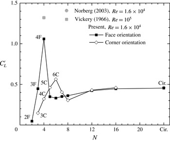
Figure 7 presents the dependence of the fluctuating lift coefficient
 $C_{L}^{\prime }$
on
 $N$
. In order to avoid the influence of the synchronisation between vortex shedding and the natural frequency of the cylinder, the
 $C_{L}^{\prime }$
measurement is limited to
 $U_{\infty }$
at which
 $f_{s}<80$
Hz. The data at
 $Re=1.6\times 10^{4}$
are illustrated. A number of observations can be made. Firstly, the present
 $C_{L}^{\prime }$
on the circular cylinder agrees very well with Norberg (Reference Norberg2003), which provides a validation for our measurements. Secondly, for either orientation,
 $C_{L}^{\prime }$
rises rapidly first with increasing
 $N$
, reaching the maximum at 4F and 6C, respectively, and then drops quickly before approaching the value of
 $N=\infty$
. Finally,
 $C_{L}^{\prime }$
varies greatly from one orientation to the other for
 $N<7$
but has the same value for both orientations for
 $N\geqslant 12$
, implying that
 $C_{L}^{\prime }$
becomes independent of the cylinder orientation for large
 $N$
. The result is consistent with the proposed analogy between the polygonal cylinder of
 $N\geqslant 12$
and the roughened circular cylinder.
Dependence of the lift coefficient
 $C_{L}^{\prime }$
on
 $N$
. Note that the data of the circular cylinder from Norberg (Reference Norberg2003) are also included, which collapse almost completely with the present measurement.

3.3 Wake characteristics
In this section, a number of wake characteristic length scales are extracted from the time-averaged velocity fields obtained from the PIV data. The length scales are further used to define the wake Strouhal number and the wake drag coefficient.
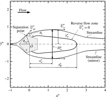
Figure 8 uses the 5C case to illustrate the definitions of wake length scales, where asterisks denote normalisations by
 $D$
and/or
 $U_{\infty }$
. One important quantity is the flow separation angle
 $\unicode[STIX]{x1D703}_{s}$
, which is defined as the angle between
 $U_{\infty }$
and
 $\overline{U}_{sp}^{\ast }$
, where
 $\overline{U}_{sp}^{\ast }$
is the tangential velocity at the separation point along the separation streamline. For the 5C case, the two angles
 $\unicode[STIX]{x1D703}_{o}$
(the separation point location) and
 $\unicode[STIX]{x1D703}_{s}$
are related by:
 $$\begin{eqnarray}\unicode[STIX]{x1D703}_{s}=\unicode[STIX]{x03C0}-(\unicode[STIX]{x1D703}_{o}+\unicode[STIX]{x1D711}/2)=\unicode[STIX]{x03C0}/2+\unicode[STIX]{x03C0}/N-\unicode[STIX]{x1D703}_{o},\end{eqnarray}$$
where
 $\unicode[STIX]{x1D711}=(N-2)\unicode[STIX]{x03C0}/N$
. The general relation of
 $\unicode[STIX]{x1D703}_{s}$
to the geometry and the orientation is not so straightforward. Note that the separation angle is defined differently from Tropea et al. (Reference Tropea, Yarin and Foss2007), where
 $\unicode[STIX]{x1D703}_{o}$
is defined as the separation angle. The reason for this different definition and a more detailed discussion of
 $\unicode[STIX]{x1D703}_{s}$
will be given in § 3.4. The marked streamlines pass through the separation points, which are also the free streamlines closest to the centreline. The reversed flow zone, defined by
 $\overline{U}_{x}^{\ast }=0$
, is marked by the streamline passing through the wake stagnation point located at
 $x_{R}^{\ast }$
downstream of the polygon centroid
 $O$
. The maximum wake width
 $D_{w}^{\ast }$
is measured at
 $x_{w}^{\ast }$
downstream of
 $O$
.
 $\overline{U}_{w}^{\ast }$
is the tangential velocity at the maximum wake width point (
 $x_{w}^{\ast },y_{w}^{\ast }$
) along the streamline through the separation point.
Definitions of various characteristic length and velocity scales in the dimensionless form for polygonal cylinder wake. Asterisks denote normalisations by
 $D$
and/or
 $U_{\infty }$
. Note that the free streamlines and reversed flow zone are drawn based on the PIV data obtained at
 $Re=1.0\times 10^{4}$
. The bottom streamline uses the mirror image of the top one due to the shadow of the cylinder (laser illumination comes from above).

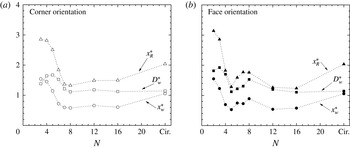
Figure 9 presents the dependences of
 $x_{R}^{\ast }$
,
 $D_{w}^{\ast }$
,
 $x_{w}^{\ast }$
on
 $N$
, which are quite similar to each other. Not surprisingly,
 $x_{R}^{\ast }\approx 2x_{w}^{\ast }$
. Different orientations result in a difference in
 $x_{R}^{\ast }$
,
 $D_{w}^{\ast }$
or
 $x_{w}^{\ast }$
, especially for
 $4\leqslant N\leqslant 8$
. Even though the blockage ratios are the same for all the cylinders, a different degree in bluffness may also have an impact on the back pressure, the separation shear layers and hence the structure of the wake (Roshko Reference Roshko1955). For
 $N\geqslant 12$
,
 $D_{w}^{\ast }$
remains roughly constant and is almost the same as that in the circular cylinder wake, but the streamwise length scales
 $x_{R}^{\ast }$
and
 $x_{w}^{\ast }$
are both significantly smaller. Note that
 $Re$
in figure 9 is well below
 $Re_{c}$
.
The dimensionless characteristic length scales (
 $x_{R}^{\ast },D_{w}^{\ast },x_{w}^{\ast }$
, defined in figure 8) as functions of
 $N$
, at
 $Re=1.0\times 10^{4}$
.

Based on the momentum equation, the drag on a bluff body can be calculated from its wake parameters (length and velocity scales) and independently on the geometry of the bluff body itself (Antonia & Rajagopalan Reference Antonia and Rajagopalan1990). Roshko (Reference Roshko1955) proposed that there exists a universal similarity for the vortex-shedding patterns and the wake structures among differently shaped bluff bodies. Once
 $(C_{p})_{b}$
is determined,
 $St^{R}$
in (1.1) is found to be
 $$\begin{eqnarray}St^{R}=\left(1-\frac{u}{U_{\infty }}\right)\left(\frac{D_{w}}{l}\right)\left(\frac{1}{\sqrt{1-(C_{p})_{b}}}\right)\approx 0.15\sim 0.17,\end{eqnarray}$$
where
 $l$
is the longitudinal vortex spacing, and
 $u$
is the convection velocity of the vortices. Williamson & Brown (Reference Williamson and Brown1998) proposed a corrected universal Strouhal number
 $St^{W}$
, viz.
 $$\begin{eqnarray}St^{W}=\left(\frac{f_{s}D}{U_{\infty }}\right)\frac{U_{\infty }}{U_{s}}\left(1+\frac{2\unicode[STIX]{x1D6FF}}{D}\right)\approx 0.176,\end{eqnarray}$$
where
 $\unicode[STIX]{x1D6FF}$
is the characteristic shear layer thickness. Ahlborn et al. (Reference Ahlborn, Seto and Noack2002) suggested another correction:
 $$\begin{eqnarray}St^{A}=\unicode[STIX]{x1D6FD}St=\left(\frac{D_{v}}{D}\right)St,\end{eqnarray}$$
where
 $D_{v}$
is the equivalent diameter of the shed vortices. The resultant universal Strouhal number from different corrections vary quite significantly, which is partly due to the ways of determining
 $D_{w}$
and
 $U_{s}$
.
The use of the above mentioned universal Strouhal number reduces and sometimes eliminates the direct influence of the bluff body geometries, though inevitably involving more quantities to be measured with more uncertainties and measurement error. For simplicity, we replace only the length scale by
 $D_{w}^{\ast }$
and define alternative
 $C_{D}^{+}$
and
 $St^{+}$
, i.e.
 $$\begin{eqnarray}\displaystyle & \displaystyle C_{D}^{+}=C_{D}/D_{w}^{\ast }, & \displaystyle\end{eqnarray}$$
 $$\begin{eqnarray}\displaystyle & \displaystyle St^{+}=StD_{w}^{\ast }=\frac{f_{s}D_{w}}{U_{\infty }}. & \displaystyle\end{eqnarray}$$
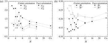
The dependences of
 $C_{D}^{+}$
and
 $St^{+}$
on
 $N$
are presented in figure 10, along with those of
 $C_{D}$
and
 $St$
. The distorted Cartesian pattern observed in figure 6 disappears for both
 $C_{D}^{+}$
and
 $St^{+}$
; rather, the data points are much less scattered. The
 $C_{D}^{+}$
data occur about 1.0 and
 $St^{+}$
near
 $0.21\sim 0.23$
, except for
 $N\leqslant 4$
. It seems plausible that using the wake scales does have potential in getting the data collapsed and in establishing a possible correlation between
 $C_{D}^{+}$
and
 $St^{+}$
(a correlation, if any, seems to be rather weak from figure 10). Nevertheless, some data points still display a relatively large scatter, especially at small
 $N$
. Note that involving the wake characteristics implies additional measurements to be conducted. It would be desirable to establish a direct correlation between
 $C_{D}$
and
 $St$
. We will propose a new scaling factor in § 3.5, which proves to work well for polygonal cylinders.
Dependence of the universal
 $C_{D}^{+}$
and
 $St^{+}$
, as compared to
 $C_{D}$
and
 $St$
, on
 $N$
.
 $Re=1.0\times 10^{4}$
.

3.4 Flow separation angle
In the context of a polygonal cylinder, the flow separation angle
 $\unicode[STIX]{x1D703}_{s}$
is in fact the angle between the particular polygon side upstream of the separation point and the incoming flow direction, that is, this angle may be directly determined from the separation point
 $\unicode[STIX]{x1D703}_{o}$
, if known. The location of
 $\unicode[STIX]{x1D703}_{o}$
and hence
 $\unicode[STIX]{x1D703}_{s}$
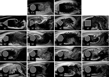
can be fairly accurately found out by carefully examining the flow visualisation images, as illustrated in figure 11. The separation points of the polygonal cylinders, including the 2F case, all occur at one of the corners (above the wake centreline), except perhaps at very large
 $N$
, such as the circular cylinder. The determined
 $\unicode[STIX]{x1D703}_{o}$
and
 $\unicode[STIX]{x1D703}_{s}$
at
 $Re=1.0\times 10^{4}$
are indicated schematically in figure 12. The
 $\unicode[STIX]{x1D703}_{s}$
for the circular cylinder is the angle between the incoming flow direction and the tangent line at the separation point. Note that, in cases of 5F and also 8C, flow separates first at corner A before reattaching to the polygon surface edge AB, and then separates again at B. Therefore, corner B is taken as the separation point.
Smoke streak flow visualisation images for all the testing cases at
 $Re=1.0\times 10^{4}$
.

Schematic diagrams indicating the location of the separation point above the centreline, marked by a circle, and the separation angle
 $\unicode[STIX]{x1D703}_{s}$
, marked by
 $\measuredangle$
, as determined at
 $Re=1.0\times 10^{4}$
.

It has been well established that
 $C_{D}$
of the circular cylinder depends on the position of the separation point. For
 $Re<Re_{c}$
, the laminar boundary layer separates fairly early, at
 $\unicode[STIX]{x1D703}_{o}\approx 79^{\circ }$
and
 $\unicode[STIX]{x1D703}_{s}\approx 11^{\circ }$
. For
 $Re>Re_{c}$
, the transition occurs in the boundary layers and the flow separation is postponed, resulting in a lower
 $C_{D}$
.
For the polygons of
 $N\leqslant 4$
,
 $\unicode[STIX]{x1D703}_{o}$
is fixed and independent of
 $Re$
.
 $C_{D}$
changes little with
 $Re$
.
For the polygons of
 $5\leqslant N\leqslant 8$
,
 $\unicode[STIX]{x1D703}_{o}$
is also fixed. To facilitate discussions, denote the point at the maximum lateral width as
 $T_{o}$
and take the front corner if two corners correspond to the maximum width position, as is the case for 6C, 8F, 12F and 16F (figure 12). Use
 $T_{1}$
and WSP to represent the corner upstream of
 $T_{o}$
and the windward stagnation point on the centreline, respectively. Four scenarios have been observed:
-
(i) flow separates at
$T_{o}$
and there is no corner between
$T_{o}$
and WSP, as for the cases for 5C, 6C and
$N\leqslant 4$
, which are associated with the dashed line 3C–5C in figure 6; -
(ii) flow separates at
$T_{o}$
and there is one corner between
$T_{o}$
and WSP (6F, 7F, 8F); -
(iii) flow separates at
$T_{1}$
and the boundary layer reattaches and separates again just before
$T_{o}$
(5F, 8C); -
(iv) flow separates at
$T_{1}$
but does not reattach (7C).


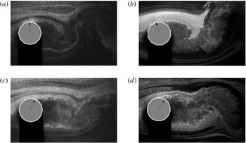
For
 $N\geqslant 12$
, the wake pattern is similar to that behind the circular cylinder, where the transition may have a pronounced effect on the flow. Nevertheless at
 $Re<Re_{c}$
, the separation point is fixed at one corner. A few examples of flow around the polygonal cylinders of
 $N\geqslant 12$
at
 $Re=5.0\times 10^{4}$
when the transition occurs (refer to figure 4) are shown in figure 13.
Smoke streak flow visualisation for (a) 12C, (b) 12F, (c) 16C and (d) 16F when the transition occurs.
 $Re=5.0\times 10^{4}$
. The arrows indicate the approximate mean separation point, since instantaneously the separation point oscillates from one instant to the next.

The dependence of
 $\unicode[STIX]{x1D703}_{s}$
on
 $N$
shows again a distorted Cartesian mesh pattern (not shown) similar to figure 6, which suggests a relation between
 $C_{D}$
and
 $\unicode[STIX]{x1D703}_{s}$
. As a matter of fact,
 $\unicode[STIX]{x1D703}_{s}$
and
 $C_{D}$
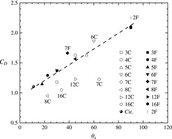
fall approximately on a linear correlation for most of the cases, as shown in figure 14. There are only a few cases that deviate from this linear correlation. It is found that the separation point occurs at
 $T_{o}$
(see figures 11 and 12) for all the cases reasonably following the linear correlation. For 7F and 8C cases,
 $T_{o}$
is actually the separation point of the reattached flow which initially separated at
 $T_{1}$
. For these two cases, the flow is more sensitive to
 $Re$
and the data
 $(\unicode[STIX]{x1D703}_{s},C_{D})$
deviate from the linear relation in figure 14. The other three data points which deviate further correspond to the cases 7C, 12C and 16C, where the flow separates at
 $T_{1}$
without reattachment. In the cases showing large deviation to the linear relation, the lateral distance between the two separation points (above and below the centreline) is not the same as the characteristic length scale
 $D$
.
Correlation between
 $C_{D}$
and
 $\unicode[STIX]{x1D703}_{s}$
at
 $Re=1.0\times 10^{4}$
.

In order to account for such deviations, we propose to define a new angle
 $\unicode[STIX]{x1D709}$
associated with the point
 $T_{o}$
, between two directions:
-
(i) the direction from
$T_{1}$
to
$T_{o}$
and the incoming flow direction in the absence of the transition; -
(ii) the direction from
$T_{o}$
to TP (the point where the transition occurs) and the incoming flow direction when the transition occurs (if TP is downstream of
$T_{o}$
,
$\unicode[STIX]{x1D709}$
is negative); -
(iii) the tangent line at the separation point and the incoming flow direction for the circular cylinder case.


Thus defined,
 $\unicode[STIX]{x1D709}$
is underpinned by two observations: (i) in the absence of the transition,
 $C_{D}$
depends only on
 $N$
and the orientation, not on
 $Re$
; (ii)
 $T_{o}$
essentially defines the entire windward surface, which effectively describes the degree of bluffness for a regular polygon of any
 $N$
. In the absence of the transition,
 $\unicode[STIX]{x1D709}$
can be mathematically written, in units of degrees, as:
 $$\begin{eqnarray}\unicode[STIX]{x1D709}=\frac{180}{\unicode[STIX]{x03C0}}\times \left\{\begin{array}{@{}ll@{}}\displaystyle \frac{\unicode[STIX]{x03C0}}{2}-\left(p-\frac{1}{2}\right)\left(\frac{2\unicode[STIX]{x03C0}}{N}\right),\quad p=\left\lceil \frac{N-2}{4}\right\rceil , & \text{NC cases;}\\ \displaystyle \frac{\unicode[STIX]{x03C0}}{2}-(q-1)\left(\frac{2\unicode[STIX]{x03C0}}{N}\right),\quad q=\left\lceil \frac{N}{4}\right\rceil , & \text{NF cases,}\end{array}\right.\end{eqnarray}$$
where
 $\lceil \,\rceil$
denotes the nearest larger integer. Note that
 $\unicode[STIX]{x1D709}$
is calculated based on
 $T_{o}$
above the centreline, which is not always the separation point. Therefore,
 $\unicode[STIX]{x1D709}$
is sometimes different from
 $\unicode[STIX]{x1D703}_{s}$
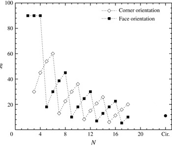
. Figure 15 presents the results calculated from (3.8), which displays a distorted Cartesian pattern similar to that in figure 6(a); see the dashed lines. When
 $Re\geqslant Re_{c}$
, for
 $N=12$
and
 $N=16$
cases,
 $\unicode[STIX]{x1D709}$
depends also on
 $Re$
and no analytical solution can be obtained simply on the geometry and orientation. The true value of
 $\unicode[STIX]{x1D709}$
when the transition occurs can be measured from experiments. It is worth mentioning that beyond
 $Re_{c}$
, the separation point is no longer fixed at a particular point; rather it oscillates around a mean location, which is determined from the average of the 100 smoke streak images.
Dependence of the angle
 $\unicode[STIX]{x1D709}$
on
 $N$
, based on (3.8), in the absence of the transition.

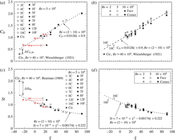
Figure 16(a) presents the dependence of
 $C_{D}$
on
 $\unicode[STIX]{x1D709}$
, which shows clearly that
 $C_{D}$
and
 $\unicode[STIX]{x1D709}$
are almost linearly related for the circular cylinder in the absence of the transition and the polygons of
 $N\leqslant 8$
. The data may be least-square-fitted to the following straight lines:
 $$\begin{eqnarray}C_{D}=0.0128\unicode[STIX]{x1D709}+0.9,\quad \text{for}~Re=(2.0\sim 10.0)\times 10^{4}.\end{eqnarray}$$
Figure 16(b) combines three
 $Re$
cases and both NC and NF orientations. The data for
 $Re=1.0\times 10^{4}$
were obtained in the wake of the polygons of
 $D=50$
mm. Evidently, the linear relation remains valid for all the data. The empirical correlation (3.9) does not take the effect of
 $Re$
into account, that is,
 $\unicode[STIX]{x1D709}$
remains the same for a given polygon in the subcritical regime and so does
 $C_{D}$
. In fact,
 $C_{D}$
for most polygons subtly decreases as
 $Re$
increases, which could be considered in (3.9) by including a
 $Re$
-related correction factor. However, this correlation term is found to be very small compared to the
 $\unicode[STIX]{x1D709}$
term, essentially within the uncertainty of (3.9). For example,
 $C_{D}$
reduces by
 ${\approx}10\,\%$
as
 $Re$
changes from
 $2.0\times 10^{4}$
to
 $1.0\times 10^{5}$
. Therefore, the
 $Re$
correction is dropped.
Dependence on
 $\unicode[STIX]{x1D709}$
of (a)
 $C_{D}$
at
 $Re=5.0\times 10^{4}$
; (b)
 $C_{D}$
at
 $Re=2.0\times ,5.0\times ,10.0\times 10^{4}$
; (c)
 $St$
at
 $Re=5.0\times 10^{4}$
; (d)
 $St$
at
 $Re=2.0\times ,5.0\times ,10.0\times 10^{4}$
. The dashed lines are the least-square-fits to the data of the circular cylinder and
 $N\leqslant 8$
in (b,d), where no transition takes place. The data obtained in the wake of a circular cylinder at
 $Re=40.0\times 10^{4}$
from Wieselsberger (Reference Wieselsberger1921) and Bearman (Reference Bearman1969) are also included for comparison. The left-pointing arrows in (a,c) illustrate the effects of the transition on the estimate of
 $\unicode[STIX]{x1D709}$
, that is,
 $\unicode[STIX]{x1D709}$
changes from the black colour symbol to the red once the transition occurs.

Figure 16(a) also reflects the importance of determining the true
 $\unicode[STIX]{x1D709}$
for the case when the transition takes place, as indicated by the left-pointing arrows. Apparently, if
 $\unicode[STIX]{x1D709}$
in the subcritical regime is used for that in the critical regime, the data points will deviate further from the fitting curve. Taking the
 $N=16$
polygon for example, the transition incurs a change in
 $\unicode[STIX]{x1D709}$
from
 $11.25^{\circ }$
to
 $-11.25^{\circ }$
for 16C and from
 $22.5^{\circ }$
to
 $-22.5^{\circ }$
for 16F. Once the correct
 $\unicode[STIX]{x1D709}$
is used, the corresponding
 $C_{D}$
collapses onto the fitting curves reasonably well, as illustrated in figure 16(b), that is, equation (3.9) may also apply to cases in the critical regime, as long as the correct
 $\unicode[STIX]{x1D709}$
is used. This implies that (3.9) can be used to predict the true separation point location and the separation angle for polygons given the flow regime.
The data from Wieselsberger (Reference Wieselsberger1921) for a circular cylinder in the critical flow regime (
 $Re=4.0\times 10^{5}$
) are also included for comparison, which deviate significantly from the fitting curve. This is not unexpected since the
 $Re$
of the data is beyond the
 $Re$
range over which the correlation is obtained.
The
 $St$
data corresponding to
 $C_{D}$
shown in figure 16(a,b) are presented in figure 16(c,d). It is obvious that the
 $St-\unicode[STIX]{x1D709}$
correlation is not quite linear and the data are least-square-fitted to a second-order polynomial, viz.
 $$\begin{eqnarray}St=7\times 10^{-6}\unicode[STIX]{x1D709}^{2}-0.00174\unicode[STIX]{x1D709}+0.222,\quad \text{for}~Re=(2.0\sim 10.0)\times 10^{4}.\end{eqnarray}$$
As shown in figure 16(c), the data collapse quite well onto this fitting curve when the correct
 $\unicode[STIX]{x1D709}$
is used. Compared to
 $C_{D}$
, the variation in
 $St$
with
 $Re$
is even smaller, within
 $\pm 4\,\%$
. Thus the
 $Re$
correction factor is also not necessary.
Empirical relation between
 $St$
and
 $C_{D}$
for all the cases tested at
 $Re=(1.0\sim 6.0)\times 10^{4}$
.
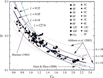
 $\unicode[STIX]{x1D701}=C_{D}^{0.6}St=0.2$
is the fitting curve based on the least-squares technique, with
 $\unicode[STIX]{x1D701}=0.22$
and 0.18 corresponding to the upper and the lower envelopes, respectively. Correlations by Hoerner (Reference Hoerner1965), Ahlborn et al. (Reference Ahlborn, Seto and Noack2002) and Alam & Zhou (Reference Alam and Zhou2008) are also included for the purpose of comparison.

Equations (3.9) and (3.10) may be used to estimate
 $C_{D}$
and
 $St$
of the untested cases. Take the 10C case for example. In the subcritical regime,
 $\unicode[STIX]{x1D709}(10\text{C})$
can be calculated from (3.8) to be
 $36^{\circ }$
. By substituting
 $\unicode[STIX]{x1D709}(10\text{C})$
into (3.9) and (3.10), we obtain
 $C_{D}(10\text{C})\approx 1.36$
and
 $St(10\text{C})\approx 0.168$
, which agree very well with the predictions in § 3.2 (figure 6).
3.5 Relation between
$C_{D}$
and
$St$


The empirical relations of equations (3.9) and (3.10) could be combined to connect directly
 $C_{D}$
and
 $St$
, although additional uncertainties may be induced as some data deviate from the fitting curves more than the others. As such, we fit, based on the least-squares technique, all the data from the measurements directly to the correlation form proposed by Hoerner (Reference Hoerner1965), viz.
 $$\begin{eqnarray}\unicode[STIX]{x1D701}=C_{D}^{0.6}St,\end{eqnarray}$$
where
 $\unicode[STIX]{x1D701}$
is a constant. Figure 17 indicates that
 $\unicode[STIX]{x1D701}=0.2$
appears to be the best fit to all the tested polygons and the
 $Re$
range (
 $1.0\times 10^{4}\sim 6.0\times 10^{4}$
). The upper and lower envelopes, given by
 $\unicode[STIX]{x1D701}=0.22$
and 0.18, enclose most of the data points except 2F, 3C and some 4C data which occur above the upper envelope. A common feature for 2F and 3C polygons is the lack of leeward body volume or afterbody leading to a higher back pressure coefficient and hence a larger
 $C_{D}\cdot St$
value (Bearman Reference Bearman1967). Using (3.11) to calculate
 $C_{D}$
from
 $St$
or vice versa yields a maximum error of approximately
 $\pm 10\,\%$
. This error may be further reduced by fine tuning the
 $\unicode[STIX]{x1D701}$
value. For example, letting
 $\unicode[STIX]{x1D701}$
to be 0.23 will enclose most of the 2F and 3C data inside the envelopes.
A number of empirical
 $C_{D}\sim St$
relations proposed by previous researchers are also plotted in figure 17 for the purpose of comparison, i.e.
 $$\begin{eqnarray}\displaystyle & 0.21=C_{D}^{0.75}St,\quad \text{Hoerner (1965)}, & \displaystyle\end{eqnarray}$$
 $$\begin{eqnarray}\displaystyle & \displaystyle k=2^{11/2}\unicode[STIX]{x03C0}\frac{C_{D}St}{C_{D}+1},\quad \text{Ahlborn}~\mathit{et~al.}~\text{(2002)}, & \displaystyle\end{eqnarray}$$
 $$\begin{eqnarray}\displaystyle & 0.23=C_{D}St,\quad \text{Alam}~\& ~\text{Zhou (2008)}, & \displaystyle\end{eqnarray}$$
where
 $k$
is an energy parameter which varies in general with different bluff body shapes. Almost all the present data, including the two envelopes (
 $\unicode[STIX]{x1D701}=0.22,0.18$
), fall between the two curves corresponding to
 $k=12$
and 16, respectively, of (3.13). Equation (3.12) does not seem to represent the present data very well for
 $C_{D}<1$
. Equation (3.14) exhibits a deviation from the data for
 $C_{D}<1$
and
 $C_{D}>2$
because this equation is derived based on the assumption of energy conservation in spite of inevitable energy exchange between the cylinder and the supporting frames in actual experiments.
It is worth making a comparison between the presently proposed (3.11) and (3.12)–(3.14) based on a collection of the data in the literature. Take
 $N=4$
and
 $N=\infty$
for example to estimate
 $St$
from
 $C_{D}$
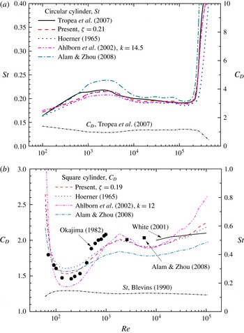
and vice versa. The results are given in figure 18. In figure 18(a) the
 $C_{D}$
data of a circular cylinder summarised in Tropea et al. (Reference Tropea, Yarin and Foss2007) are used to calculate the corresponding
 $St$
from (3.12)–(3.14). In view of the data distribution for a circular cylinder in figure 17, the
 $\unicode[STIX]{x1D701}$
value in (3.11) is chosen to be 0.21 to represent the best
 $C_{D}$
on the circular cylinder in figure 18(a). The
 $k$
value in (3.13) is chosen to be 14.5, which gives the best fit. Note that Ahlborn et al. (Reference Ahlborn, Seto and Noack2002) suggested
 $k=12.7$
, which produces a larger deviation from the experimental data. Equation (3.11), albeit obtained from the data over a limited
 $Re$
range, gives the best fit to the experimental data from Tropea et al. (Reference Tropea, Yarin and Foss2007) for a wider
 $Re$
range and is even in agreement with the data of
 $Re>Re_{c}$
. Comparing to (3.12), equation (3.11) is equally good for
 $Re<Re_{c}$
but better for
 $Re>Re_{c}$
. Equation (3.14) displays a large deviation for
 $10^{3}<Re<10^{4}$
and (3.13) agrees well with the experimental data for the entire
 $Re$
range presented, similarly to (3.11).
Evaluation of various
 $St\sim C_{D}$
relations (3.11)–(3.14): (a)
 $St$
calculated from
 $C_{D}$
on a circular cylinder summarised in Tropea et al. (Reference Tropea, Yarin and Foss2007); (b)
 $C_{D}$
calculated from
 $St$
on a square cylinder summarised in Blevins (Reference Blevins1990). Experimental data from Okajima (Reference Okajima1982), White (Reference White2001) and Alam & Zhou (Reference Alam and Zhou2008) are included for the purpose of comparison.

Figure 18(b) presents the
 $C_{D}$
data for the
 $N=4$
polygon, calculated based on (3.11) to (3.14), from
 $St$
summarised in Blevins (Reference Blevins1990). Comparison is further made between the calculated
 $C_{D}$
values and those reported in the literature. The
 $\unicode[STIX]{x1D701}$
value in (3.11) is chosen to be 0.19. In (3.13),
 $k$
is set to be 12, which leads to a better fit to the data than
 $k=11.5$
proposed in Ahlborn et al. (Reference Ahlborn, Seto and Noack2002). The
 $C_{D}$
data calculated from (3.11) agree qualitatively with the available experimental data in Okajima (Reference Okajima1982) for
 $Re<1.0\times 10^{3}$
, but increase from 1.9 to 2.2 for
 $1.0\times 10^{4}<Re<1.0\times 10^{5}$
, exceeding the experimental data reported in White (Reference White2001), with the largest deviation up to 10 %. Assessment cannot be made for other
 $Re$
ranges due to a lack of experimental data. The prediction from (3.12) is quite similar to that from (3.11).
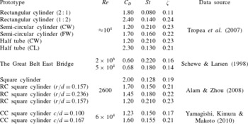
Table 2 summarises
 $C_{D}$
and
 $St$
, reported in the literature, for the two-dimensional bodies of various cross-sectional geometry or irregular bluff bodies. The
 $\unicode[STIX]{x1D701}$
value is calculated based on
 $C_{D}$
and
 $St$
from (3.11). While most bluff bodies fall in between the envelopes (
 $0.18\leqslant \unicode[STIX]{x1D701}\leqslant 0.22$
),
 $\unicode[STIX]{x1D701}$
tends to be small for more streamline-shaped bodies. For example, the rectangular cylinder with an aspect ratio 2 : 1 corresponds to
 $\unicode[STIX]{x1D701}=0.11$
, smaller than 0.24, with an aspect ratio of 1 : 2. Table 2 and also figure 18 indicate that
 $\unicode[STIX]{x1D701}$
is independent of
 $Re$
for cylinders with mild bluffness, at least for the
 $Re$
range examined presently. Furthermore, the experimental data (not shown) confirm that
 $\unicode[STIX]{x1D701}$
changes in the range of
 $0.20\pm 0.02$
as the angle of attack of the polygonal cylinder varys between the corner and the face orientations at
 $Re=5.0\times 10^{4}$
.
The
 $C_{D}$
and
 $St$
values of various irregular polygonal cylinders reported in the literature and their correlation coefficient
 $\unicode[STIX]{x1D701}$
calculated from (3.11). In the table, CW, FW and CL denote the windward-facing curved surface, the windward-facing flat surface and the leeward-facing curved surface, respectively; RC and CC represent the rounded corner and the chamfered corner, respectively;
 $r$
,
 $d$
and
 $c$
are the abbreviations for the radius of the rounded corner, the side length of the square cylinder and the size of the chamfered corner, respectively.

Figure 17 indicates that
 $St$
and
 $C_{D}$
are inversely related. This can be demonstrated analytically.
Assuming that the vortices shed from the cylinders are two-dimensional and can be approximately described by the Lamb–Oseen vortex model (Saffman Reference Saffman1995), the azimuthal velocity
 $u_{\unicode[STIX]{x1D703}}$
of an isolated vortex can be written as:
 $$\begin{eqnarray}\displaystyle u_{\unicode[STIX]{x1D703}}(r_{s},t)=\frac{\unicode[STIX]{x1D6E4}_{o}}{2\unicode[STIX]{x03C0}r_{s}}\left[1-\exp \left(-\frac{r_{s}^{2}}{4\unicode[STIX]{x1D708}t}\right)\right],\end{eqnarray}$$
where
 $t$
is time (
 $\sqrt{4\unicode[STIX]{x1D708}t}$
is the characteristic vortex size),
 $\unicode[STIX]{x1D6E4}_{o}$
is the vortex strength and
 $r_{s}$
is the radius to the vortex centre. The kinetic energy of the flow field associated with an isolated Lamb–Oseen vortex may be written as:
 $$\begin{eqnarray}\displaystyle \mathit{KE} & = & \displaystyle \int _{0}^{\infty }\unicode[STIX]{x1D70C}\unicode[STIX]{x03C0}r_{s}u_{\unicode[STIX]{x1D703}}^{2}\,\text{d}r_{s}\nonumber\\ \displaystyle & = & \displaystyle \unicode[STIX]{x1D70C}\frac{\unicode[STIX]{x1D6E4}_{o}^{2}}{4\unicode[STIX]{x03C0}}\int _{0}^{\infty }\frac{1}{r_{s}}\left[1-2\exp \left(-\frac{r_{s}^{2}}{4\unicode[STIX]{x1D708}t}\right)+\exp \left(-\frac{2r_{s}^{2}}{4\unicode[STIX]{x1D708}t}\right)\right]\text{d}r,\end{eqnarray}$$
where
 $\unicode[STIX]{x1D70C}$
is the fluid density. From the energy budget point of view, one pair of vortices form over one period of vortex shedding, which produces a drag force
 $F_{D}$
, i.e.
 $KE=F_{D}U_{\infty }\unicode[STIX]{x1D70F}$
, where
 $\unicode[STIX]{x1D70F}=D/U_{\infty }$
is the characteristic time scale of vortex shedding. Defining a dimensionless circulation
 $K=\unicode[STIX]{x1D6E4}_{o}/\unicode[STIX]{x03C0}U_{\infty }D$
and writing the integral in (3.16) as
 $\unicode[STIX]{x1D702}(t)$
,
 $C_{D}$
is then related to
 $St$
as:
 $$\begin{eqnarray}C_{D}=\unicode[STIX]{x03C0}K^{2}St\unicode[STIX]{x1D702}(t).\end{eqnarray}$$
The formation of a vortex is the roll up of a shear layer, and vortex shedding occurs when fluid engulfed in carrying vorticity with opposite signs cuts off further the entrainment of circulation (Gerrard Reference Gerrard1966). Taking the average velocity in the boundary layer to be
 $U_{\infty }/2$
and
 $\unicode[STIX]{x1D6FF}$
to be the characteristic boundary layer thickness, consider a shear layer with vorticity
 $\unicode[STIX]{x1D714}\sim U_{\infty }/\unicode[STIX]{x1D6FF}$
rolling up over time
 $\unicode[STIX]{x1D70F}$
. Then
 $$\begin{eqnarray}K\sim \frac{1}{\unicode[STIX]{x03C0}DU_{\infty }}\left(\frac{U_{\infty }}{\unicode[STIX]{x1D6FF}}\right)(\unicode[STIX]{x1D6FF}\unicode[STIX]{x1D70F}U_{\infty }/2)=\left(\frac{1}{2\unicode[STIX]{x03C0}}\right)St^{-1}.\end{eqnarray}$$
Note that, depending on the degree of bluffness and hence the wake width, only a fraction of the circulation contributes to the vortex formation (Bearman Reference Bearman1984). Equation (3.18) then needs to be revised such that
 $$\begin{eqnarray}K\sim \frac{1}{\unicode[STIX]{x03C0}DU_{\infty }}\left(\frac{U_{\infty }}{\unicode[STIX]{x1D6FF}}\right)(\unicode[STIX]{x1D6FF}\unicode[STIX]{x1D70F}U_{\infty }/2)f(D_{w}^{\ast })=\frac{f(D_{w}^{\ast })}{2\unicode[STIX]{x03C0}}St^{-1}.\end{eqnarray}$$
The
 $Re$
effect may be reflected in
 $D_{w}^{\ast }$
. Substituting (3.19) into (3.17) yields
 $$\begin{eqnarray}C_{D}=\frac{1}{4\unicode[STIX]{x03C0}St}\,f(D_{w}^{\ast })\unicode[STIX]{x1D702}(t).\end{eqnarray}$$
The integrand of
 $\unicode[STIX]{x1D702}(t)$
is bounded over
 $r_{s}\in [0,\infty )$
and the integral
 $\unicode[STIX]{x1D702}(t)$
is not very sensitive to
 $t$
. Therefore,
 $\unicode[STIX]{x1D702}(t)$
is a weak function of the characteristic vortex size
 $\sqrt{4\unicode[STIX]{x1D708}t}$
. Taking a realistic vortex size to be of the order of
 $D/2$
,
 $\unicode[STIX]{x1D702}$
is typically around 7.0. Substituting the known numerical values into
 $f$
, we may finally obtain
 $$\begin{eqnarray}C_{D}=f(D_{w}^{\ast })St^{-1}.\end{eqnarray}$$
As the empirical correlation (3.11) agrees well with the present experimental data, we may infer
 $f(D_{w}^{\ast })\sim \unicode[STIX]{x1D701}C_{D}^{-0.4}$
. Note that
 $C_{D}$
is an increasing function of
 $D_{w}^{\ast }$
, that is,
 $C_{D}$
increases with larger
 $D_{w}^{\ast }$
. Using the
 $D_{w}^{\ast }$
data at
 $Re=1.0\times 10^{4}$
shown in figure 9 and the corresponding
 $C_{D}$
, we may find
 $D_{w}^{\ast }\sim C_{D}^{0.8}$
. Therefore,
 $f(D_{w}^{\ast })\sim (D_{w}^{\ast })^{-1/2}$
.
4 Concluding remarks
The aerodynamic characteristics of polygonal cylinders (
 $N=2,3\sim 8$
, 12, 16,
 $\infty$
) are systematically studied over a
 $Re$
range of
 $1.0\times 10^{4}\sim 1.0\times 10^{5}$
, based on the three-dimensional force transducer, smoke flow visualisation and PIV measurements. Both corner and face orientations of the polygonal cylinders are examined. The following conclusions may be drawn from this work.
It has been found that
 $C_{D}$
,
 $C_{L}^{\prime }$
and
 $St$
all vary with
 $N$
as well as with the polygon orientation. The dependence of
 $C_{D}$
on
 $N$
exhibits a distorted Cartesian pattern (figure 6
a,b). So does that of
 $St$
on
 $N$
(figure 6
c,d). This pattern may be used to predict
 $C_{D}$
and
 $St$
for untested polygons, e.g.
 $N=9\sim 11$
. In general,
 $C_{D}$
,
 $C_{L}^{\prime }$
and
 $St$
all depend on the polygon orientation. This dependence however contracts with increasing
 $N$
. While
 $C_{L}^{\prime }$
becomes independent of the polygon orientation for
 $N\geqslant 12$
,
 $C_{D}$
and
 $St$
may differ, albeit very slightly, from one polygon orientation to the other. The characteristic length scales of the wake, such as the wake width and the length of the reversed flow region and their dependence on
 $N$
are also documented.
The present flow visualisation data (figure 11) show unequivocally that, given polygons of
 $N\leqslant 8$
, the flow separation point is fixed at the corner of the maximum width point
 $T_{o}$
. As such,
 $C_{D}$
and
 $St$
change little, essentially independently of
 $Re$
(see also figure 4). In a few cases, e.g. 5F and 7C, although separating at corner
 $T_{1}$
, upstream of
 $T_{o}$
, the flow reattaches near
 $T_{o}$
, again resulting in
 $C_{D}$
and
 $St$
that are independent of
 $Re$
. The cylinders of N12 and N16 undergo the transition at
 $Re_{c}\approx 2.4\times 10^{4}$
and
 ${\approx}3.4\times 10^{4}$
, respectively; correspondingly,
 $C_{D}$
drops substantially, accompanied by a large increase in
 $St$
. Once the transition takes place, the flow separation is postponed, allowing more recovery in pressure; the energised boundary layer due to the transition enhances the shear layer instability, causing relatively small-scale vortices to be generated at higher frequencies.
One of the most important findings of this study is the corrected flow separation angle
 $\unicode[STIX]{x1D709}$
, which has essentially taken the separation–reattachment phenomenon into account. This angle is uniquely dependent on the orientation and
 $N$
of the polygon in the subcritical regime (figure 15), i.e.
 $Re<Re_{c}$
. More importantly, the dependence of
 $C_{D}$
or
 $St$
, which is greatly scattered if plotted against
 $N$
(figure 6) or other parameters, on
 $\unicode[STIX]{x1D709}$
collapses onto a single curve as shown in figure 16, even under the circumstance of the transition, implying that
 $\unicode[STIX]{x1D709}$
is a scaling factor for both
 $C_{D}$
and
 $St$
. The correlation between
 $C_{D}$
and
 $\unicode[STIX]{x1D709}$
is even linear. This finding allows us to predict the
 $C_{D}$
and
 $St$
of the polygonal cylinder from
 $\unicode[STIX]{x1D709}$
from a careful flow visualisation experiment, without the need for the force transducer of high dynamic response or hot-wires. The linear correlation between
 $\unicode[STIX]{x1D709}$
and
 $C_{D}$
is perhaps not surprising. Ahlborn et al. (Reference Ahlborn, Seto and Noack2002) showed that
 $C_{D}$
is linearly proportional to
 $\tan \unicode[STIX]{x1D703}$
, where
 $\unicode[STIX]{x1D703}$
is the angle between the transverse velocity and the streamwise velocity of vortices separated from the cylinder. Yeung (Reference Yeung2009) found a linear relation between
 $C_{D}$
and
 $(C_{p})_{b}$
for some bluff bodies such as cones and spheres. The definition of
 $\unicode[STIX]{x1D709}$
is essentially related to
 $\unicode[STIX]{x1D703}$
and
 $(C_{p})_{b}$
on the polygon; once the transition takes place,
 $\unicode[STIX]{x1D709}$
characterises uniquely the location of the flow separation point. If the direction of
 $U_{s}$
(see § 3.3, related to the geometry of the polygon) is considered,
 $\unicode[STIX]{x1D703}_{s}$
and hence
 $(C_{p})_{b}$
can be inferred from
 $\unicode[STIX]{x1D709}$
.
It has been found that
 $Re_{c}$
rises for larger
 $N$
given
 $N\geqslant 12$
(figure 5
a). An analogy, in terms of
 $Re_{c}$
, between the polygons of
 $N\geqslant 12$
and the rough surface circular cylinders, is proposed. The corners of these polygons act like the roughness elements, with a height
 $\unicode[STIX]{x1D700}$
calculated by (3.1), evenly distributed on the surface of a smooth circular cylinder. The dependence of
 $Re_{c}$
on
 $\unicode[STIX]{x1D700}/D$
follows well both qualitatively and quantitatively the dependence of
 $Re_{c}$
on the relative roughness of a roughened circular cylinder (figure 5). As a result,
 $Re_{c}$
for the untested polygons of large
 $N$
may be predicted from the well documented
 $Re_{c}$
of the rough surface circular cylinder. However, for
 $N<12$
, the size and number of ‘the roughness elements’ become relatively large and small, respectively, and the corners cannot be treated as roughness elements anymore and the analogy is no longer valid.
The one-to-one correlation between
 $C_{D}$
and
 $\unicode[STIX]{x1D709}$
and that between
 $St$
and
 $\unicode[STIX]{x1D709}$
imply a relation between
 $C_{D}$
and
 $St$
. A new empirical correlation is proposed, i.e.
 $\unicode[STIX]{x1D701}=C_{D}^{0.6}St$
, and the best fit to the present experimental data as well as those in the literature is
 $\unicode[STIX]{x1D701}=0.20$
. When
 $\unicode[STIX]{x1D701}=0.22$
and
 $\unicode[STIX]{x1D701}=0.18$
, the corresponding curves form two envelopes that enclose most of the available experimental data points. This relationship is found to be valid not only for the polygonal cylinders but also the bluff bodies of irregular cross-section over
 $Re=50\sim 10^{6}$
.
Finally, we have demonstrated analytically that
 $C_{D}$
and
 $St$
are inversely related, as shown by the experimental data in figure 17.
Acknowledgements
S.J.X. wishes to acknowledge the support from NSFC through grants 10972118 and 11472158. L.G. would like to thank the support from the United Kingdom Royal Society of Engineering Newton Research Collaboration Fund (NRCP/1415/130). Y.Z. is grateful for the financial support from NSFC through grant 51421063 and from Scientific Research Fund of Shenzhen Government through grant KQCX20140521144301394. The authors also acknowledge Professor Z. N. Wu of Tsinghua University for his constructive discussions.