1 Introduction
The Lagrangian approach is widely used for the analysis of mixing processes. It relies on the tracking of individual fluid particles and provides important information on the flow kinematics and stirring features of a given flow. The emergence of very complicated fluid trajectories leading to Lagrangian chaos, even in rather simple time-dependent laminar flows, lies on the foundations of chaotic advection (Aref Reference Aref1984, Reference Aref2002; Aref et al. Reference Aref, Blake, Budii, Cartwright, Clercx, Feudel, Golestanian, Gouillart, Le Guer and van Heijst2017). The large number of applications that involve mixing of low-Reynolds-number flows, particularly in microfluidics, has motivated the search for methods to perform the stirring process in efficient and controlled ways. The use of electromagnetic forces has proved to be a convenient non-intrusive method to generate vortices (Cruz-Gómez, Zavala-Sansón & Pinilla Reference Cruz-Gómez, Zavala-Sansón and Pinilla2013) and to stir electrically conducting fluids, particularly electrolytes (Yi, Qian & Bau Reference Yi, Qian and Bau2002). The main idea is to apply an electric current in a thin layer of electrolyte exposed to either a uniform magnetic field or a magnetic field created by an external array of permanent magnets, in such a way that rotational Lorentz forces are produced. Many fundamental mixing-related problems have been explored with this technique in shallow layers of electrolytic fluids, for instance, the response of shear flows to a constant injection of energy in a confined domain (González-Vera & Zavala-Sansón Reference González-Vera and Zavala-Sansón2015) or the generation of turbulent-like flows, namely, laminar multiscale flows with turbulent properties (Rossi, Vassilicos & Hardalupas Reference Rossi, Vassilicos and Hardalupas2006a ,Reference Rossi, Vassilicos and Hardalupas b ). Electromagnetic forces have also been used to generate chaotic quasi-two-dimensional flows in which time-dependent stretching fields (Voth, Haller & Gollub Reference Voth, Haller and Gollub2002), mixing rates (Voth et al. Reference Voth, Saint, Dobler and Gollub2003), as well as topological features of the flow (e.g. time-dependent elliptic and hyperbolic points) have been experimentally determined (Ouellete & Gollub Reference Ouellete and Gollub2007). On the other hand, quasi-steady flows driven by electromagnetic forces have been used to illustrate lamination, that is, the ensemble of processes that build striated structures (Rossi Reference Rossi2010; Rossi & Lardeau Reference Rossi and Lardeau2011; Rossi, Doorly & Kustrin Reference Rossi, Doorly and Kustrin2012, Reference Rossi, Doorly and Kustrin2013). Based on the interlaced nature of velocity and the Lagrangian acceleration, it is possible to quantify lamination rates and determine the spatial variation of the Lagrangian angular velocity. These studies take advantage of the versatility of electromagnetic forces to be tailored in order to generate a sequential mixing protocol. Recently, laminar mixing at large Péclet numbers was explored experimentally and theoretically in flows driven by oscillating electromagnetic forces in a thin layer of electrolyte (Figueroa et al. Reference Figueroa, Meunier, Cuevas, Villermaux and Ramos2014). In this study, the advection–diffusion problem was addressed through numerical simulations based on the diffusive strip method (DSM) (Meunier & Villermaux Reference Meunier and Villermaux2010), which combines Lagrangian techniques and theoretical modelling of the diffusion. Numerical simulations obtained with the DSM showed reasonable agreement with quantitative dye visualization experiments of the scalar fields. Further, theoretical modelling allowed the prediction of the probability density functions (p.d.f.s) of the scalar field in agreement with numerical and experimental results.
While a suitable combination of stretching and folding may produce exponential growth of material interfaces and a corresponding mixing enhancement, the existence of symmetries may inhibit good mixing. In the case of electromagnetically driven flows, symmetries may be promoted by an ordered array of magnets that generate a symmetrical distribution of the magnetic field. Different strategies can be implemented to break the symmetries and enhance mixing, for instance, by using a disordered array of magnets (Voth et al. Reference Voth, Saint, Dobler and Gollub2003) or by increasing the intensity of the applied current with an ordered array (Ouellete & Gollub Reference Ouellete and Gollub2007; Ouellette & Gollub Reference Ouellette and Gollub2008). A less common strategy was implemented by Solomon et al. (Reference Solomon, Winokur, O’Malley and Paoletti2008), who explored vortices created by Lorentz forces in an ordered array of magnets. A square array of vortices was obtained by applying a current parallel to one of the primary directions of the magnet array. When the current is tilted with respect to the magnet array, wavy channels formed diagonally through the vortex pattern. When an alternating current (AC) was applied in both cardinal directions, a barrier-free chaotic mixing was found.
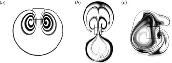
In the present work, we explore a strategy similar to that of Solomon et al. (Reference Solomon, Winokur, O’Malley and Paoletti2008) but focusing attention on the Lagrangian trajectories created when two orthogonal localized Lorentz forces act on a thin electrolytic layer. We restrict the analysis to laminar quasi-two-dimensional vortices created with a single magnet in order to show that, even in this simple case, rather complex trajectories can be obtained. It is well known that a one-directional direct current (DC) interacting with the field created by a single dipole magnet generates a steady vortex dipole (see figure 1 a). In turn, if the current is AC, an oscillating vortex dipole is formed (see figure 1 b). In both cases, symmetrical vortex patterns, with a symmetry line defined by the direction of the applied force, appear due to the uniformity of the applied current and the dipolar magnetic field distribution. These observations have been described in Figueroa et al. (Reference Figueroa, Demiaux, Ramos and Cuevas2009, Reference Figueroa, Meunier, Cuevas, Villermaux and Ramos2014) and Figueroa, Cuevas & Ramos (Reference Figueroa, Cuevas and Ramos2011). Here, we show that the action of two orthogonal time-periodic Lorentz forces breaks the symmetry of the flow created by a unidirectional driving force (see figure 1 c). We call this flow pattern a Lissajous vortex since it produces Lagrangian trajectories similar to the well-known Lissajous figures. These figures were observed in 1855 by Jules Antoine Lissajous, who devised a simple optical method for studying compound vibrations. He found complex patterns formed when two harmonic vibrations along perpendicular lines are superimposed. As long as the ratio of the two perturbing frequencies is a rational number, no matter how complex, the curve will eventually repeat itself, causing the motion to be periodic. Instead, if the frequency ratio is irrational, the curve will never retrace its own path, resulting in a non-periodic motion and, as time progresses, the curve will gradually fill the domain (Pook Reference Pook2011). Incidentally, in 1871 Boltzmann made the analogy between physical trajectories of particles in two-dimensional space and Lissajous figures, which appears to be Boltzmann’s first description of the ergodic hypothesis (Nolte Reference Nolte2010). While Lissajous figures can be understood from a purely kinematic and non-dissipative point of view, Lagrangian trajectories studied here originate from a dissipative nonlinear system, namely, an electromagnetically driven viscous flow. We employ analytical, numerical and experimental approaches to explore the behaviour of the Lagrangian trajectories at low Reynolds numbers. As has been experimentally demonstrated and numerically verified, for restricted Reynolds numbers vortical structures produced by electromagnetic forcing with either DC (Figueroa et al. Reference Figueroa, Demiaux, Ramos and Cuevas2009) or AC (Figueroa et al. Reference Figueroa, Cuevas and Ramos2011, Reference Figueroa, Meunier, Cuevas, Villermaux and Ramos2014) currents remain quasi-two-dimensional. In fact, it will be shown that the analysed flows comply with the quasi-two-dimensionality criterion proposed by Durán-Matute et al. (Reference Durán-Matute, Kamp, Trieling and van Heijst2010). In a recent report, Baskan et al. (Reference Baskan, Speetjens, Metcalfe and Clercx2015) present experimental evidence that validates that the motion of passive tracers advected in two-dimensional unsteady flows can be described as a Hamiltonian system. The flow studied was generated by moving sections of the walls that confine a shallow layer of liquid (rotated arc mixer). The results presented here on Lagrangian tracking share some features with the study of Baskan et al. (Reference Baskan, Speetjens, Metcalfe and Clercx2015) but with the difference that our driving force is volumetric (Lorentz force) rather than the application of surface forces at the boundaries. First, by considering a weak inertial regime, we use a perturbation method to get an analytical two-dimensional solution for the velocity field from which Lagrangian trajectories are integrated explicitly. In this regime, Lagrangian trajectories reproduce the typical properties of Lissajous figures related with the periodicity and non-periodicity of the motion for rational and irrational frequency ratios, respectively. In order to explore nonlinear effects on the flow behaviour, a quasi-two-dimensional numerical solution is implemented. In this case, trajectories present drastic changes with respect to classical Lissajous figures displaying non-closed paths even for rational frequency ratios. The description is complemented with time maps that show chaotic behaviour for a rational frequency ratio, as the Reynolds number is increased. Further, numerically calculated Lagrangian trajectories and time maps for one single particle are compared with experimental results based on particle tracking.
Experimental visualization of vortex flows generated by electromagnetic forcing. The steady (a) and oscillating (b) vortex dipoles are obtained, respectively, when DC or AC currents applied in the horizontal direction interact with the field produced by a permanent dipolar magnet. In turn, Lissajous vortex (c) results from AC currents, applied in the horizontal and vertical directions, interacting with the field of the permanent magnet. In case (b) the forcing frequency in the horizontal direction is 50 mHz. In case (c) forcing frequencies in the horizontal and vertical directions are 50 mHz with a relative phase shift of
 $\unicode[STIX]{x1D719}=\unicode[STIX]{x03C0}/2$
. The square denotes the footprint of the magnet.

2 Experimental set-up and methodology
The experimental set-up used in the investigation reported here presents slight variations with respect to the one described in detail in Figueroa et al. (Reference Figueroa, Demiaux, Ramos and Cuevas2009, Reference Figueroa, Cuevas and Ramos2011). Essentially, it consists of a rectangular container partially filled with a thin layer of electrolyte, namely, a solution of sodium bicarbonate (NaHCO
 $_{3}$
) at 8.6 % by weight. The length, width and depth of the electrolyte layer are 36 cm, 28 cm and 0.4 cm, respectively, with a total volume of
 $400~\text{cm}^{3}$
. At room temperature, the mass density, kinematic viscosity and electrical conductivity of the electrolyte are
 $\unicode[STIX]{x1D70C}=1.09\times 10^{3}~\text{kg}~\text{m}^{-3}$
,
 $\unicode[STIX]{x1D708}=10^{-6}~\text{m}^{2}~\text{s}^{-1}$
and
 $\unicode[STIX]{x1D70E}=6.36~\text{S}~\text{m}^{-1}$
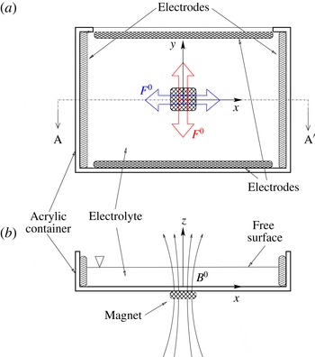
, respectively. Unlike the previous set-up, where only one pair of copper electrodes are used, in the present set-up two pairs of electrodes are placed along the inner borders of the container, taking care to avoid short circuits (see figure 2). Each pair of electrodes is connected to a Stanford Research System DS345 function generator for obtaining independent electrical signals that allow one to modify the frequency and the phase of the signals. Oscillatory electric currents with frequencies ranging from 10 to 30 mHz are applied through the electrodes. By the use of a potentiometer, the amplitudes of the applied electric currents are modulated to
 $I=1~\text{mA}$
. At this current intensity, electrolysis is very small. The origin of the coordinate system is placed in the geometrical centre of the container at the bottom wall, so that the
 $x$
and
 $y$
coordinates lie on the horizontal plane of the frame, while the
 $z$
coordinate points in the normal direction. A squared parallelepiped neodymium magnet with a side length of 50.8 mm and height of 25.4 mm is placed under the container at (
 $x=0,~y=0$
). The magnet is vertically magnetized and the maximum strength at its surface is 0.38 T. Experimental visualizations with dye were performed by depositing a blob of disodium fluorescein (with molecular diffusivity
 $D=5\times 10^{-10}~\text{m}^{2}~\text{s}^{-1}$
) on the electrolyte layer. Quantitative measurements of the velocity field on the flow plane at
 $z=3.5~\text{mm}$
were obtained with a particle image velocimetry system (Dantec FlowMap PIV1100). We obtained 40 velocity fields per cycle with a spatial resolution of 0.86 mm, and 10 cycles were averaged. In addition, particle tracking was performed using a flat plastic coloured disc of 0.5 mm radius floating on the surface of the fluid layer. The fluid domain was photographed every 2 s with a Nikon D90 camera with an AF Micro-Nikkor 60 mm f/2.8D lens.
Sketch of the experimental device, not drawn to scale: (a) plan view, and (b) cross-sectional AA
 $^{\prime }$
plane. Within the layer, the magnetic field
 $B^{0}$
points mainly in the positive
 $z$
direction. The main directions of the Lorentz forces are denoted by
 $F^{0}$
. The Lorentz forces in red and in blue are generated by the interaction of the applied electric currents through the vertically and horizontally aligned electrodes, respectively, and the magnetic field. The square denotes the footprint of the magnet.

3 Theoretical model
Flows in weak electrolytes driven by Lorentz forces can be modelled using the continuity and Navier–Stokes equations with the Lorentz force as a source term (Figueroa et al. Reference Figueroa, Demiaux, Ramos and Cuevas2009, Reference Figueroa, Cuevas and Ramos2011; Figueroa Reference Figueroa2010). In dimensionless form, the governing equations read
 $$\begin{eqnarray}\displaystyle & \unicode[STIX]{x1D735}\boldsymbol{\cdot }\boldsymbol{u}=0, & \displaystyle\end{eqnarray}$$
 $$\begin{eqnarray}\displaystyle & \displaystyle R_{\unicode[STIX]{x1D714}}\frac{\unicode[STIX]{x2202}\boldsymbol{u}}{\unicode[STIX]{x2202}t}+(\boldsymbol{u}\boldsymbol{\cdot }\unicode[STIX]{x1D735})\boldsymbol{u}=-\unicode[STIX]{x1D735}p+\unicode[STIX]{x1D6FB}^{2}\boldsymbol{u}+Re\,\boldsymbol{j}^{0}\times \boldsymbol{B}^{0}, & \displaystyle\end{eqnarray}$$
where the velocity field
 $\boldsymbol{u}$
is normalized by
 $u_{0}=\unicode[STIX]{x1D708}/L$
,
 $\unicode[STIX]{x1D708}$
and
 $L$
denoting the kinematic viscosity of the fluid and the side length of the magnet, respectively; the pressure field,
 $p$
, is normalized by
 $\unicode[STIX]{x1D70C}u_{0}^{2}$
, where
 $\unicode[STIX]{x1D70C}$
is the mass density of the fluid; coordinates are normalized by
 $L$
and time is normalized by
 $1/\unicode[STIX]{x1D714}$
, where
 $\unicode[STIX]{x1D714}=2\unicode[STIX]{x03C0}f$
is the angular frequency and
 $f$
is the ordinary frequency obtained from the average of both electric current frequencies. The last term on the right-hand side of (3.2) considers the oscillating Lorentz force created by the non-uniform magnetic field distribution of the permanent magnet,
 $\boldsymbol{B}^{0}=\boldsymbol{B}^{0}(x,y,z)$
, which is normalized by its maximum strength,
 $B_{max}$
, and the applied current densities in the
 $x$
and
 $y$
directions, namely,
 $\boldsymbol{j}^{0}=J_{x}\sin (\unicode[STIX]{x1D6FA}_{x}t)\,\hat{\boldsymbol{x}}+J_{y}\sin (\unicode[STIX]{x1D6FA}_{y}t+\unicode[STIX]{x1D719})\,\hat{\boldsymbol{y}}$
, where
 $J_{x}=j_{x}/j^{0}$
and
 $J_{y}=j_{y}/j^{0}$
, with
 $j_{x}$
and
 $j_{y}$
being the current density amplitudes in the
 $x$
and
 $y$
directions, respectively. Here, the applied current density amplitude is defined as
 $j^{0}=I/A$
, where
 $A$
is the cross-sectional area. The dimensionless angular frequencies of the applied current are denoted by
 $\unicode[STIX]{x1D6FA}_{x}=f_{x}/f$
and
 $\unicode[STIX]{x1D6FA}_{y}=f_{y}/f$
, and the relative phase shift of the electrical signals is
 $\unicode[STIX]{x1D719}$
. The two governing parameters,
 $Re=U_{0}L/\unicode[STIX]{x1D708}$
and
 $R_{\unicode[STIX]{x1D714}}=\unicode[STIX]{x1D714}L^{2}/\unicode[STIX]{x1D708}$
, are the Reynolds and oscillation Reynolds numbers, respectively. The characteristic bulk velocity
 $U_{0}=j^{0}B_{max}L^{2}/\unicode[STIX]{x1D70C}\unicode[STIX]{x1D708}$
is obtained from a balance between viscous and Lorentz forces (Figueroa et al.
Reference Figueroa, Demiaux, Ramos and Cuevas2009). It is worth mentioning that for electrolyte and liquid metal flows in laboratory conditions, the magnetic Reynolds number,
 $R_{m}=\unicode[STIX]{x1D707}_{0}\unicode[STIX]{x1D70E}U_{0}L$
, where
 $\unicode[STIX]{x1D707}_{0}$
is the magnetic permeability, is much less than unity, which implies that the induced field is much smaller than the applied field. In the present experiment,
 $R_{m}$
is of order
 $10^{-10}$
. If the conducting fluid were a liquid metal, currents induced by the fluid motion should be considered and (3.1) and (3.2) should be complemented with the induction equation for the induced magnetic field.
3.1 Two-dimensional analytical solution
In the present subsection, an analytical solution of (3.1) and (3.2) in the creeping flow regime (
 $Re\ll 1$
and
 $R_{\unicode[STIX]{x1D714}}\ll 1$
) is derived. To do so, we introduce some simplifying assumptions. First, we assume that the flow is two-dimensional and takes place in an infinite domain
 $-\infty <x<\infty$
,
 $-\infty <y<\infty$
. The variation in the
 $z$
direction is not taken into account. Therefore, the effects of the bottom wall and the free surface are disregarded. Under these conditions, only the component of the applied magnetic field normal to the plane of motion is relevant, namely
 $B_{z}^{0}(x,y)$
, which is assumed to be produced by a point magnetic dipole. Since the experimental system does not comply with these conditions, the comparison of experimental results with the idealized model can only reach the qualitative level. With these assumptions, the governing equations reduce to
 $$\begin{eqnarray}\displaystyle & \displaystyle \frac{\unicode[STIX]{x2202}u}{\unicode[STIX]{x2202}x}+\frac{\unicode[STIX]{x2202}v}{\unicode[STIX]{x2202}y}=0, & \displaystyle\end{eqnarray}$$
 $$\begin{eqnarray}\displaystyle & \displaystyle R_{\unicode[STIX]{x1D714}}\frac{\unicode[STIX]{x2202}u}{\unicode[STIX]{x2202}t}+u\frac{\unicode[STIX]{x2202}u}{\unicode[STIX]{x2202}x}+v\frac{\unicode[STIX]{x2202}u}{\unicode[STIX]{x2202}y}=-\frac{\unicode[STIX]{x2202}p}{\unicode[STIX]{x2202}x}+\unicode[STIX]{x1D6FB}_{\bot }^{2}u+Re\,j_{y}^{0}B_{z}^{0}, & \displaystyle\end{eqnarray}$$
 $$\begin{eqnarray}\displaystyle & \displaystyle R_{\unicode[STIX]{x1D714}}\frac{\unicode[STIX]{x2202}v}{\unicode[STIX]{x2202}t}+u\frac{\unicode[STIX]{x2202}v}{\unicode[STIX]{x2202}x}+v\frac{\unicode[STIX]{x2202}v}{\unicode[STIX]{x2202}y}=-\frac{\unicode[STIX]{x2202}p}{\unicode[STIX]{x2202}y}+\unicode[STIX]{x1D6FB}_{\bot }^{2}v-Re\,j_{x}^{0}B_{z}^{0}, & \displaystyle\end{eqnarray}$$
where the subscript
 $\bot$
indicates the projection of the
 $\unicode[STIX]{x1D735}$
operator on the
 $(x,y)$
plane,
 $j_{x}^{0}(t)=J_{x}\sin (\unicode[STIX]{x1D6FA}_{x}t)$
and
 $j_{y}^{0}(t)=J_{y}\sin (\unicode[STIX]{x1D6FA}_{y}t+\unicode[STIX]{x1D719})$
. Upon taking the curl of (3.4) and (3.5), we get the following vorticity transport equation for the only component
 $\unicode[STIX]{x1D714}_{z}$
:
 $$\begin{eqnarray}R_{\unicode[STIX]{x1D714}}\frac{\unicode[STIX]{x2202}\unicode[STIX]{x1D714}_{z}}{\unicode[STIX]{x2202}t}+u\frac{\unicode[STIX]{x2202}\unicode[STIX]{x1D714}_{z}}{\unicode[STIX]{x2202}x}+v\frac{\unicode[STIX]{x2202}\unicode[STIX]{x1D714}_{z}}{\unicode[STIX]{x2202}y}=\unicode[STIX]{x1D6FB}_{\bot }^{2}\unicode[STIX]{x1D714}_{z}-Re\left(j_{x}^{0}\frac{\unicode[STIX]{x2202}B_{z}^{0}}{\unicode[STIX]{x2202}x}+j_{y}^{0}\frac{\unicode[STIX]{x2202}B_{z}^{0}}{\unicode[STIX]{x2202}y}\right).\end{eqnarray}$$
We now look for an asymptotic solution as a double perturbation expansion for small values of the parameters
 $Re$
and
 $R_{\unicode[STIX]{x1D714}}$
. First, we expand the vorticity
 $\unicode[STIX]{x1D714}_{z}$
(and similarly the velocity components
 $u$
and
 $v$
) as a series in integral powers of
 $Re$
, namely,
 $$\begin{eqnarray}\unicode[STIX]{x1D714}_{z}=\unicode[STIX]{x1D714}_{z}^{(0)}+Re\,\unicode[STIX]{x1D714}_{z}^{(1)}+Re^{2}\unicode[STIX]{x1D714}_{z}^{(2)}+O(Re^{3}),\end{eqnarray}$$
where the superscript denotes the order of the approximation. Solutions of this sort become increasingly accurate as the perturbation parameter
 $Re$
gets smaller. The zeroth-order solution (
 $O(Re^{0})$
) corresponds to the fluid at rest (no currents applied). At first order (
 $O(Re)$
), the vorticity satisfies
 $$\begin{eqnarray}R_{\unicode[STIX]{x1D714}}\frac{\unicode[STIX]{x2202}\unicode[STIX]{x1D714}_{z}^{(1)}}{\unicode[STIX]{x2202}t}=\unicode[STIX]{x1D6FB}_{\bot }^{2}\unicode[STIX]{x1D714}_{z}^{(1)}-j_{x}^{0}\frac{\unicode[STIX]{x2202}B_{z}^{0}}{\unicode[STIX]{x2202}x}-j_{y}^{0}\frac{\unicode[STIX]{x2202}B_{z}^{0}}{\unicode[STIX]{x2202}y}.\end{eqnarray}$$
Now, we expand the velocity components and the vorticity as series in the small parameter
 $R_{\unicode[STIX]{x1D714}}$
. The solution at order
 $O(Re,R_{\unicode[STIX]{x1D714}}^{0})$
satisfies (quasi-steady limit)
 $$\begin{eqnarray}0=\unicode[STIX]{x1D6FB}_{\bot }^{2}\unicode[STIX]{x1D714}_{z}^{(1,0)}-j_{x}^{0}\frac{\unicode[STIX]{x2202}B_{z}^{0}}{\unicode[STIX]{x2202}x}-j_{y}^{0}\frac{\unicode[STIX]{x2202}B_{z}^{0}}{\unicode[STIX]{x2202}y}.\end{eqnarray}$$
This equation can be integrated analytically if the applied magnetic field is assumed to be a point magnetic dipole. The normal component of a two-dimensional point magnetic dipole located at the origin with its magnetic dipole moment pointing in the positive
 $z$
direction can be expressed as (Cuevas, Smolentsev & Abdou Reference Cuevas, Smolentsev and Abdou2006)
 $$\begin{eqnarray}B_{z}^{0}(x,y)=\frac{1}{2\unicode[STIX]{x03C0}}\frac{1}{x^{2}+y^{2}}+\unicode[STIX]{x1D6FF}(x)\unicode[STIX]{x1D6FF}(y).\end{eqnarray}$$
Note that the field has been normalized by
 $B_{max}=\unicode[STIX]{x1D707}_{0}m/{\mathcal{L}}^{2}$
, where
 $\unicode[STIX]{x1D707}_{0}$
and
 $m$
are the magnetic permeability and the magnetic dipole moment, respectively. In this case, the characteristic length
 ${\mathcal{L}}$
is chosen in such a way that the normalization constant takes a value of 1, that is,
 ${\mathcal{L}}=\sqrt{\unicode[STIX]{x1D707}m}$
. Equation (3.10) represents a two-dimensional magnetic point dipole. The solution of (3.9) is
 $$\begin{eqnarray}\unicode[STIX]{x1D714}_{z}^{(1,0)}=\frac{1}{2\unicode[STIX]{x03C0}}\frac{y}{x^{2}+y^{2}}\,j_{y}^{0}(t)+\frac{1}{2\unicode[STIX]{x03C0}}\frac{x}{x^{2}+y^{2}}\,j_{x}^{0}(t).\end{eqnarray}$$
Observe that
 $\lim _{x,y\rightarrow \infty }\unicode[STIX]{x1D714}_{z}^{(1,0)}=0$
, and that, although solution (3.11) presents a singularity at the origin, it reproduces correctly the vorticity in the neighbourhood of the origin. The velocity field can be obtained through the streamfunction
 $\unicode[STIX]{x1D713}$
, defined as
 $u=\unicode[STIX]{x2202}\unicode[STIX]{x1D713}/\unicode[STIX]{x2202}y$
,
 $v=-\unicode[STIX]{x2202}\unicode[STIX]{x1D713}/\unicode[STIX]{x2202}x$
, which satisfies the equation
 $$\begin{eqnarray}\unicode[STIX]{x1D6FB}_{\bot }^{2}\unicode[STIX]{x1D713}=-\unicode[STIX]{x1D714}_{z}.\end{eqnarray}$$
By expanding the streamfunction and vorticity at first order in
 $Re$
and zeroth order in
 $R_{\unicode[STIX]{x1D714}}$
, equation (3.12) becomes
 $$\begin{eqnarray}\unicode[STIX]{x1D6FB}_{\bot }^{2}\unicode[STIX]{x1D713}^{(1,0)}=-\unicode[STIX]{x1D714}_{z}^{(1,0)},\end{eqnarray}$$
whose general solution is
 $$\begin{eqnarray}\unicode[STIX]{x1D713}^{(1,0)}=\left(\frac{x}{8\unicode[STIX]{x03C0}}\,j_{x}^{0}(t)-\frac{y}{8\unicode[STIX]{x03C0}}\,j_{y}^{0}(t)\right)(\ln (x^{2}+y^{2})-1)+C_{1}\frac{x+y}{x^{2}+y^{2}}+C_{2}(x+y).\end{eqnarray}$$
Choosing
 $C_{1}=C_{2}=0$
, we get
 $$\begin{eqnarray}\unicode[STIX]{x1D713}^{(1,0)}=\left(\frac{x}{8\unicode[STIX]{x03C0}}\,j_{x}^{0}(t)+\frac{y}{8\unicode[STIX]{x03C0}}\,j_{y}^{0}(t)\right)(1-\ln (x^{2}+y^{2})).\end{eqnarray}$$
Using the same methodology, the following solutions at higher orders (i.e.
 $O(Re^{1},R_{\unicode[STIX]{x1D714}}^{1})$
and
 $O(Re^{2},R_{\unicode[STIX]{x1D714}}^{0})$
) can be obtained:
 $$\begin{eqnarray}\unicode[STIX]{x1D713}^{(1,1)}=\frac{x^{2}+y^{2}}{128\unicode[STIX]{x03C0}}(5-2\ln (x^{2}+y^{2}))(xj_{x}^{0}(t)\unicode[STIX]{x1D6FA}_{x}+yj_{y}^{0}(t)\unicode[STIX]{x1D6FA}_{y}),\end{eqnarray}$$
 $$\begin{eqnarray}\displaystyle \unicode[STIX]{x1D713}^{(2,0)} & = & \displaystyle \frac{1}{512\unicode[STIX]{x03C0}^{2}}\left(\ln (x^{2}+y^{2})-(\ln (x^{2}+y^{2}))^{2}-\frac{1}{2}\right)\nonumber\\ \displaystyle & & \displaystyle \times \,(xy(j_{x}^{0}(t))^{2}-(x^{2}-y^{2})j_{x}^{0}(t)j_{y}^{0}(t)-xy(j_{y}^{0}(t))^{2}).\end{eqnarray}$$
Finally, the approximate solution reads
 $$\begin{eqnarray}\unicode[STIX]{x1D713}(x,y,t)=Re^{0}\unicode[STIX]{x1D713}^{0}+Re^{1}(R_{\unicode[STIX]{x1D714}}^{0}\unicode[STIX]{x1D713}^{(1,0)}+R_{\unicode[STIX]{x1D714}}^{1}\unicode[STIX]{x1D713}^{(1,1)})+Re^{2}(R_{\unicode[STIX]{x1D714}}^{0}\unicode[STIX]{x1D713}^{(2,0)}).\end{eqnarray}$$
Note that the term
 $O(Re^{2})$
introduces small nonlinear effects. The divergence at
 $r\rightarrow 0$
and
 $r\rightarrow \infty$
reveals a problem intrinsic to the approximation
 $Re\ll 1$
. Nevertheless, as shown in § 4, solution (3.18) provides a suitable approximation in intermediate regions.
Once the components of the velocity field are known, the coordinates of passive tracer particles can be found by integrating the (dimensionless) advective equations
 $$\begin{eqnarray}R_{\unicode[STIX]{x1D714}}\frac{\text{d}x}{\text{d}t}=u(x,y,t),\quad R_{\unicode[STIX]{x1D714}}\frac{\text{d}y}{\text{d}t}=v(x,y,t).\end{eqnarray}$$
For the approximate two-dimensional analytical solution, velocity components are obtained from the streamfunction (3.18). In this case, equation (3.19) can be integrated explicitly for given initial conditions. Numerical integration of the advection equations will also be provided for velocity fields calculated numerically through a quasi-two-dimensional model that simulates the electromagnetically driven flow with a finite size magnet.
3.2 Quasi-two-dimensional numerical model
In order to simulate the experimental flows where nonlinear effects are present, a quasi-two-dimensional numerical model for
 $Re>1$
and
 $R_{\unicode[STIX]{x1D714}}>1$
was used, like the one presented in Figueroa et al. (Reference Figueroa, Demiaux, Ramos and Cuevas2009, Reference Figueroa, Meunier, Cuevas, Villermaux and Ramos2014) and Figueroa (Reference Figueroa2010). The quasi-two-dimensional model is based on averaging the balance equations in the normal
 $z$
direction so that flows are described in terms of two-dimensional core flow with a linear friction that accounts for the effects of the oscillating boundary layer. The model considers the magnetic field created by a finite magnet and its decay in the normal direction. In dimensionless terms, the averaged governing equations in the (
 $x,y$
) plane read
 $$\begin{eqnarray}\displaystyle & \displaystyle \frac{\unicode[STIX]{x2202}u}{\unicode[STIX]{x2202}x}+\frac{\unicode[STIX]{x2202}v}{\unicode[STIX]{x2202}y}=0, & \displaystyle\end{eqnarray}$$
 $$\begin{eqnarray}\displaystyle & \displaystyle R_{\unicode[STIX]{x1D714}}\frac{\unicode[STIX]{x2202}u}{\unicode[STIX]{x2202}t}+u\frac{\unicode[STIX]{x2202}u}{\unicode[STIX]{x2202}x}+v\frac{\unicode[STIX]{x2202}u}{\unicode[STIX]{x2202}y}=-\frac{\unicode[STIX]{x2202}p}{\unicode[STIX]{x2202}x}+\unicode[STIX]{x1D6FB}_{\bot }^{2}u-\frac{u}{\unicode[STIX]{x1D70F}}+\unicode[STIX]{x1D6FC}\,Re\,j_{y}^{0}B_{z}^{0}, & \displaystyle\end{eqnarray}$$
 $$\begin{eqnarray}\displaystyle & \displaystyle R_{\unicode[STIX]{x1D714}}\frac{\unicode[STIX]{x2202}v}{\unicode[STIX]{x2202}t}+u\frac{\unicode[STIX]{x2202}v}{\unicode[STIX]{x2202}x}+v\frac{\unicode[STIX]{x2202}v}{\unicode[STIX]{x2202}y}=-\frac{\unicode[STIX]{x2202}p}{\unicode[STIX]{x2202}y}+\unicode[STIX]{x1D6FB}_{\bot }^{2}v-\frac{v}{\unicode[STIX]{x1D70F}}-\unicode[STIX]{x1D6FC}\,Re\,j_{x}^{0}B_{z}^{0}. & \displaystyle\end{eqnarray}$$
Here,
 $B_{z}^{0}$
reproduces the variation of the field in the (
 $x,y$
) plane using an analytical expression for the field of a magnetized rectangular surface uniformly polarized in the normal direction (McCaig Reference McCaig1977). In order to reproduce the magnetic field of the permanent magnet, the superposition of two parallel magnetized square surfaces with opposing polarization axes was considered (Figueroa et al.
Reference Figueroa, Demiaux, Ramos and Cuevas2009). Coordinates
 $x$
and
 $y$
are normalized by the characteristic side length
 $L$
of the magnet, while coordinate
 $z$
is normalized by the depth of the layer
 $h$
. Note that both (3.21) and (3.22) contain a Lorentz force term and the linear friction term, called Rayleigh friction, which involves a characteristic dimensionless time scale,
 $\unicode[STIX]{x1D70F}$
, for the damping of vorticity due to dissipation in the viscous layers at the bottom wall, and whose inverse is given by
 $$\begin{eqnarray}\unicode[STIX]{x1D70F}^{-1}=\text{Re}\left\{\frac{a\,\text{sinh}(\sqrt{a}\unicode[STIX]{x1D716}^{2})+\sqrt{a}\unicode[STIX]{x1D6FE}(\text{e}^{-\unicode[STIX]{x1D6FE}\unicode[STIX]{x1D716}^{2}}-\text{cosh}(\sqrt{a}\unicode[STIX]{x1D716}^{2}))}{{\displaystyle \frac{\unicode[STIX]{x1D6FE}\text{e}^{-\unicode[STIX]{x1D6FE}\unicode[STIX]{x1D716}^{2}}}{\sqrt{a}}}(\text{cosh}(\sqrt{a}\unicode[STIX]{x1D716}^{2})-1)-\text{sinh}(\sqrt{a}\unicode[STIX]{x1D716}^{2})-{\displaystyle \frac{\sqrt{a}}{\unicode[STIX]{x1D6FE}}}\text{cosh}(\sqrt{a}\unicode[STIX]{x1D716}^{2})(\text{e}^{-\unicode[STIX]{x1D6FE}\unicode[STIX]{x1D716}^{2}}-1)}\right\},\end{eqnarray}$$
where
 $a=\text{i}R_{\unicode[STIX]{x1D714}}$
. Here,
 $\unicode[STIX]{x1D700}=h/L$
is the aspect ratio that compares the characteristic lengths in the normal and transverse directions and
 $\text{Re}$
indicates the real part of the expression inside the brackets
 $\{~\}$
. According to the shallow flow approximation,
 $\unicode[STIX]{x1D700}$
is assumed to be less than unity (in the experiment, the value of
 $\unicode[STIX]{x1D700}$
is 0.08). The quantity
 $\unicode[STIX]{x1D70F}^{-1}$
comes from considering that viscous layers at the bottom wall behave like an oscillating Stokes velocity profile (Figueroa et al.
Reference Figueroa, Cuevas and Ramos2011). Further, owing to the variation of the magnetic field in the normal direction, the Lorentz force terms in (3.21) and (3.22) include the attenuation factor
 $\unicode[STIX]{x1D6FC}$
given by (Figueroa et al.
Reference Figueroa, Demiaux, Ramos and Cuevas2009)
 $$\begin{eqnarray}\unicode[STIX]{x1D6FC}=\int _{0}^{\unicode[STIX]{x1D700}}\exp (-\unicode[STIX]{x1D6FE}\unicode[STIX]{x1D700}z)\,\text{d}z,\end{eqnarray}$$
where
 $\unicode[STIX]{x1D6FE}=1.64$
was obtained from experimental measurements. The coefficient
 $\unicode[STIX]{x1D6FE}$
is related to the decaying of the magnetic field in the vertical direction, as explained with detail in Figueroa et al. (Reference Figueroa, Cuevas and Ramos2011). The system of equations (3.20)–(3.22), complemented with the friction model (3.23), the factor
 $\unicode[STIX]{x1D6FC}$
(3.24) and the distribution of the applied magnetic field (
 $B_{z}^{0}$
), was solved numerically using a finite difference method (Cuevas et al.
Reference Cuevas, Smolentsev and Abdou2006) in a bounded domain of the same size as that of the experiment, and assuming that velocity components satisfy no-slip conditions at the boundaries of the container.
4 Results
When a single AC electric current is applied in the
 $x$
direction, the Lorentz force generates a dipole vortex that oscillates in the
 $y$
direction (Figueroa et al.
Reference Figueroa, Cuevas and Ramos2011) and remains symmetric as long as both parameters
 $Re$
and
 $R_{\unicode[STIX]{x1D714}}$
are small. When
 $Re$
is increased, vortices are advected along the
 $y$
axis, in the direction of the main Lorentz force. When transverse currents are applied in the
 $x$
and
 $y$
directions, for small values of
 $Re$
and
 $R_{\unicode[STIX]{x1D714}}$
the resulting flow pattern is the superposition of two transverse vortex dipoles. For increasing values of these parameters, more complex phenomena arise. In fact, unexpected flow patterns can appear from the combination of the electrical parameters, namely the amplitude, frequency and phase shift of each current, particularly when inertial effects come into play, as described in detail in the next subsections.
4.1 Lagrangian trajectories due to Lissajous vortices in creeping flow regime
Let us explore the Lagrangian trajectories in the creeping flow limit for different cases that involve rational frequency ratios. For all cases presented in this subsection, both Reynolds and oscillation Reynolds numbers take small values (
 $Re\ll 1$
and
 $R_{\unicode[STIX]{x1D714}}\ll 1$
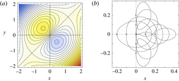
). For each case, the instantaneous streamlines at different times are first presented in order to illustrate the corresponding Eulerian flow field. For instance, figure 3(a) shows the instantaneous streamlines calculated from the analytical solution when both frequencies are equal and the phase shift between currents is
 $\unicode[STIX]{x03C0}/2$
. The Eulerian flow field consists of an oscillating dipole vortex that rotates due to the resulting anticlockwise rotating Lorentz force. Note that the analytical solution, calculated with the idealized case of a point dipole magnet, predicts a perfectly symmetric dipole vortex due to negligible inertial effects.
Analytical calculations for
 $\unicode[STIX]{x1D6FA}_{x}=1$
,
 $\unicode[STIX]{x1D6FA}_{y}=1$
,
 $\unicode[STIX]{x1D719}=\unicode[STIX]{x03C0}/2$
,
 $Re\ll 1$
and
 $R_{\unicode[STIX]{x1D714}}\ll 1$
. (a) Instantaneous streamlines of Lissajous vortex (
 $t=\unicode[STIX]{x03C0}/4$
). (b) Lagrangian trajectories in the Lissajous vortex calculated from analytic integration of advection equations. Crosses (
 $\times$
) denote the initial position of the tracers.

As expected, the corresponding Lagrangian trajectories for this flow are strongly dependent on the initial condition. Figure 3(b) shows the trajectories obtained from the explicit analytic integration of advection equations (3.19) for different starting points. If a passive tracer is placed at the geometrical centre of the flow domain (
 $x=0,~y=0$
), in one period the particle describes an approximately circular curve that resembles the corresponding Lissajous figure when both forcing frequencies are equal and the phase shift is
 $\unicode[STIX]{x03C0}/2$
. As the initial position of the tracer is moved from the origin, the trajectory is distorted but it always closes after one period.
We now consider the numerically calculated flow produced by a finite size dipole magnet interacting with two orthogonal currents in phase (
 $\unicode[STIX]{x1D719}=0$
) with a rational frequency ratio (
 $\unicode[STIX]{x1D6FA}_{x}=8$
,
 $\unicode[STIX]{x1D6FA}_{y}=9$
). In this case, even with the small values of
 $Re$
and
 $R_{\unicode[STIX]{x1D714}}$
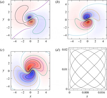
, the instantaneous streamlines at different times show an oscillating vortex dipole that rotates anticlockwise while being distorted by small inertial effects (see figure 4
a–c). The Lagrangian trajectory obtained from the integration of the advection equations when the tracer is initially placed at the origin is presented in figure 4(d). It resembles again the corresponding Lissajous figure. Results obtained with the analytical solution compare qualitatively well also for this case. In a similar manner as figure 3(b), as the initial position is moved from the origin, the path of the tracer is distorted. In fact, very complex (although closed) trajectories are found.
Instantaneous streamlines of Lissajous vortex calculated numerically when the magnetic source is a finite size dipole magnet, for
 $\unicode[STIX]{x1D6FA}_{x}=8$
,
 $\unicode[STIX]{x1D6FA}_{y}=9$
,
 $\unicode[STIX]{x1D719}=0$
,
 $Re=0.1$
and
 $R_{\unicode[STIX]{x1D714}}=0.1$
: (a)
 $t=6\unicode[STIX]{x03C0}/20$
, (b)
 $t=16\unicode[STIX]{x03C0}/20$
and (c)
 $t=31\unicode[STIX]{x03C0}/20$
. (d) Lagrangian trajectory in the Lissajous vortex when the initial position of the tracer is the origin.

As long as the frequency ratio
 $\unicode[STIX]{x1D6FA}_{x}/\unicode[STIX]{x1D6FA}_{y}$
is a rational number, the path of the tracer will describe a closed curve, that is, it will eventually repeat itself, causing the motion to be periodic. Analogously to Lissajous figures for an irrational frequency ratio, the Lagrangian trajectory is no longer a closed curve. The tracer performs a non-periodic motion so that the curve progressively covers an area that depends on the frequencies involved; the larger the frequencies, the smaller the area.
4.2 Inertial effects on Lagrangian trajectories of Lissajous vortices
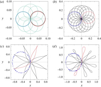
The Lagrangian trajectories observed when inertial effects are present are no longer closed independently of whether the frequency ratio is rational or irrational, hence, a fluid particle will never retrace its own path. Figure 5 shows that small inertial effects drastically alter the trajectories. A tracer released near the origin of coordinates is acted upon by orthogonal forces dephased by
 $\unicode[STIX]{x03C0}/2$
but with the same frequency, i.e. with unity frequency ratio. The oscillatory Reynolds number is
 $R_{\unicode[STIX]{x1D714}}=0.1$
. For
 $Re=0.05$
the tracer orbit is a quasi-circular non-closed path in one forcing period, shown in red in figure 5(a). After several periods, the trajectory describes a set of tight quasi-circular loops (only a few cycles are shown in black for clarity), the centres of which rotate anticlockwise uniformly. This effect can be appreciated from the sample orbits shown in green. A geometrical model of the orbits can be easily identified. Specifically, the orbit in figure 5(a) describes an epicycloid (Lemaire Reference Lemaire1967; Lawrence Reference Lawrence1972) of the form
 $$\begin{eqnarray}x=\unicode[STIX]{x1D705}\cos (\unicode[STIX]{x1D711})-\unicode[STIX]{x1D706}\cos (\unicode[STIX]{x1D709}\unicode[STIX]{x1D711}),\quad y=\unicode[STIX]{x1D705}\sin (\unicode[STIX]{x1D711})-\unicode[STIX]{x1D706}\sin (\unicode[STIX]{x1D709}\unicode[STIX]{x1D711}),\end{eqnarray}$$
where the parameter
 $\unicode[STIX]{x1D711}$
is a real number greater than or equal to zero,
 $\unicode[STIX]{x1D705}$
and
 $\unicode[STIX]{x1D706}$
are small numbers and
 $\unicode[STIX]{x1D709}$
is an irrational number. We used
 $\unicode[STIX]{x1D705}$
,
 $\unicode[STIX]{x1D706}\sim 0.4$
and
 $\unicode[STIX]{x1D709}=0.01/\sqrt{2}$
to closely reproduce the orbits of figure 5(a). Increasing the Reynolds number to
 $Re=0.2$
(figure 5
b), an oval non-closed path is traced in one period. The corresponding geometrical model is also an epicycloid with
 $\unicode[STIX]{x1D705}$
,
 $\unicode[STIX]{x1D706}\sim 0.15$
and
 $\unicode[STIX]{x1D709}=0.085/\sqrt{2}$
. For
 $Re=1.0$
and
 $Re=1.4$
(figure 5
c,d), the trajectories depart drastically from the quasi-circular path and extend to a larger area. For these higher Reynolds numbers, we found that most of the geometrical properties can be represented by hypotrochoids.
Small inertial effects on Lagrangian trajectories calculated numerically for a Lissajous vortex with a rational frequency ratio, for
 $\unicode[STIX]{x1D6FA}_{x}=1$
,
 $\unicode[STIX]{x1D6FA}_{y}=1$
,
 $\unicode[STIX]{x1D719}=\unicode[STIX]{x03C0}/2$
and
 $R_{\unicode[STIX]{x1D714}}=0.1$
: (a)
 $Re=0.05$
, (b)
 $Re=0.2$
, (c)
 $Re=1.0$
and (d)
 $Re=1.4$
. The green lines in (a) are sample orbits. In (a–d) the black lines are the Lagrangian trajectories, whereas the red lines display the trajectory in one period. Blue points denote the time maps for 160 periods.

We can make a further analysis of the geometrical properties of the orbits using time maps (also called
 $T$
maps) by sampling the flow at discrete times using a time interval
 $T$
. With this technique, the continuous orbit yields a sequence of points (see Ott (Reference Ott1993) for a formal description and properties of time maps). Before we embark on the description of the maps, it is pertinent to indicate that the time map of the linear creeping flow where the orbits are described by harmonic functions is just a set of discrete points. If the time interval is taken as
 $T=1/f$
, the time map coincides with the initial position of tracers, denoted by the small crosses in figure 3(b). When weak inertial effects are incorporated in the analysis, using the same time interval
 $1/f$
, the time map for orbits whose initial positions are close to the origin is a distribution of points on a circle centred at a point located on the
 $x$
axis and that tangentially touches the origin. This is illustrated by the blue circle superposed in figure 5(a) for the case
 $Re=0.05$
,
 $R_{\unicode[STIX]{x1D714}}=0.1$
. Observe that the distribution of points is not centred at the origin because of the initial conditions chosen for the numerical integration. When the Reynolds number is increased, two effects on the time map are observed: a radial perturbation on the circular disposition and the clustering of points in some azimuthal regions, i.e. the incremental angle between consecutive points is no longer constant. The sets of dots in figure 5(b–d) illustrate this effect.
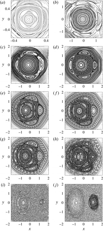
Time maps of the evolution of the Lagrangian flow topology for
 $400T$
due to Lissajous vortex with parameters
 $\unicode[STIX]{x1D6FA}_{x}=1$
,
 $\unicode[STIX]{x1D6FA}_{y}=1$
and
 $\unicode[STIX]{x1D719}=\unicode[STIX]{x03C0}/2$
: (a)
 $Re=0.05$
, (b)
 $Re=0.1$
, (c)
 $Re=0.2$
, (d)
 $Re=0.4$
, (e)
 $Re=0.8$
, (f)
 $Re=0.9$
, (g)
 $Re=1$
, (h)
 $Re=1.4$
, (i)
 $Re=5$
and (j)
 $Re=10$
. Two-dimensional numerical calculation;
 $R_{\unicode[STIX]{x1D714}}=0.1$
.

Figure 6 shows the evolution of the time maps taking the Reynolds number as the parameter. The individual panels were built using 800 initial points uniformly distributed and 400 periods were considered. Both injected currents have the same frequency but their signals are shifted
 $\unicode[STIX]{x03C0}/2$
. The maps in figure 6 range from a perturbation to the linear case in figure 6(a) where the influence of the nonlinear terms is small, to the nearly stochastic distribution of points in the map of figure 6(j). The sequence shares many features with Poincaré maps of area-preserving Hamiltonian models. See, for example, the evolution of the standard or Chirikov map as the control parameter is increased (Jackson Reference Jackson1991). In figure 6(a) we display the map that corresponds to the same parameters used to calculate figure 5(a) but in an area 25 times larger. This can be interpreted as a perturbation to the linear solution, which can be identified with the integrable case of area-preserving Hamiltonians. Recall that the slightly asymmetrical distribution of points is due to the initial conditions used. Two alternating regions according to the point distribution can be identified. For
 $|x|,\,|y|<0.2$
, the points arrange themselves in approximately circular patterns. Then, for
 $0.2<|x|,\,|y|<0.35$
, the point distributions can be identified as squares with the vertices aligned with the axes of coordinates. In the region
 $0.35<|x|,\,|y|<0.5$
, the points form again approximately circular patterns. This circle–square pattern alternates in regions further away from the origin of the axes of coordinates. The maps obtained for perturbations of the integrable systems can be further characterized using the concept of rotation number
 ${\mathcal{R}}$
defined as (Baskan et al.
Reference Baskan, Speetjens, Metcalfe and Clercx2015):
 $$\begin{eqnarray}{\mathcal{R}}(x_{0})=\lim _{P\rightarrow \infty }\frac{1}{P}\frac{\displaystyle \mathop{\sum }_{p=0}^{P-1}\unicode[STIX]{x0394}\unicode[STIX]{x1D703}_{p}}{2\unicode[STIX]{x03C0}},\end{eqnarray}$$
where
 $\unicode[STIX]{x1D703}_{p}$
is the azimuthal position of the
 $p$
point, and
 $\unicode[STIX]{x0394}\unicode[STIX]{x1D703}_{p}=\unicode[STIX]{x1D703}_{p}-\unicode[STIX]{x1D703}_{p+1}$
. The rotation number describes the average stepwise rotation of a tracer about the origin. By definition
 ${\mathcal{R}}>0$
and
 ${\mathcal{R}}<0$
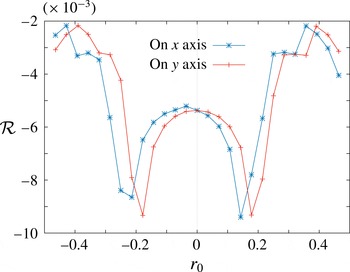
for clockwise and anticlockwise rotation, respectively. Figure 7 shows the distribution of
 ${\mathcal{R}}$
for
 $Re=0.05$
and
 $R_{\unicode[STIX]{x1D714}}=0.1$
(figure 6
a), as a function of the initial positions of the tracers. The blue and red lines denote the tracers whose initial positions are located at a distance
 $r_{0}$
along the
 $x$
and
 $y$
axes, respectively. We can observe symmetry for
 ${\mathcal{R}}$
with respect to the line
 $r_{0}=0$
in the
 $y$
direction. The
 ${\mathcal{R}}$
trace obtained for initial positions in the
 $x$
direction has a small offset due to the initial conditions of the numerical integration. As can be appreciated, the regions where the rotation number increases as the seeding point moves away from the coordinate axis coincide with the circular distribution of points in the time map, namely
 $|x|,\,|y|<0.2$
. Conversely, in the regions where the rotation number becomes smaller as the distance from the origin of coordinates increases (
 $0.2<|x|,\,|y|<0.35$
), the point distribution corresponds to the tilted square distribution of points in figure 6(a). In figure 6(c), two important features can be noticed. In the regions close to
 $x^{2}+y^{2}=1$
, a clear set of four hyperbolic points interspaced with elliptic points can be identified, while in the inner region, a chain of 19 hyperbolic–elliptic points are found. The occurrence of these structures have been profusely described and interpreted for the case of Poincaré sections of area-preserving Hamiltonians (Jackson Reference Jackson1991; Ott Reference Ott1993; José & Saletan Reference José and Saletan1998). As the Reynolds number increases, the sets of elliptic and hyperbolic points appear in concentric regions, and zones of stochastic distribution of points are found in regions that were occupied by hyperbolic points in maps of smaller Reynolds numbers. The emergence of chains of hyperbolic and elliptic points based on circular structures as the Reynolds number is increased is very similar to the corresponding evolution in area-preserving Hamiltonian models and for small
 $Re$
can be interpreted as a consequence of rotation number gradients. Observe that there is an even number of hyperbolic (and elliptic) points as described by the Poincaré–Birkhoff theorem (Jackson Reference Jackson1991). Regarding figure 6(d), the time maps for particles seeded in the strong magnetic field zone show well-defined circular distributions that increase their radius to an interface limit where the time map presents four elliptical zones connected with hyperbolic points. This zone is surrounded with not well-defined circular distributions. The well-defined shapes occur in low-velocity zones, whereas blurred shapes occur in high-velocity zones. As the Reynolds number is increased, the internal circular shapes are deformed to elliptical structures and even new elliptical zones appear. The outer original elliptical zones are shortened and elongated till they practically disappear. Figure 6(h) presents small elliptic islands around a large one. The identification of collections of points that hint at similar structures to those found in the theory suggests that the underlying fundamental mechanisms that drive the Lagrangian dynamics are the same, to the extent that the experiment approximates a two-dimensional flow.
Tracer dynamics near the integrable limit (
 $Re=0.05$
,
 $R_{\unicode[STIX]{x1D714}}=0.1$
) investigated by the rotation number
 ${\mathcal{R}}$
. The initial tracer position is on the
 $x$
axis or the
 $y$
axis at a distance
 $r_{0}$
from the origin.

4.3 Comparison of numerical Lagrangian trajectories with experimental particle tracking
The tracking of a single particle was implemented experimentally with the aim of observing Lagrangian trajectories and comparing their general features with the trajectories calculated with the numerical model. Experimentally, particle tracking has severe limitations due to the difficulty of finding tracers that behave approximately as advective (passive) particles. As mentioned in § 2, a coloured flat piece of plastic with a circular shape (0.5 mm radius) floating on the free surface of the liquid layer was used as a tracer. The tracer was photographed every 2 s as it was conveyed by the flow during one forcing period so that a clear trajectory is defined. Moreover, only a single tracer was tracked since two or more adhered and formed clusters, which strongly disturb the original velocity field.
Before the theoretical and experimental Lagrangian properties of the flows were compared, a validation of the Eulerian velocity field calculated with the code was made. Velocity fields calculated with the parameters used in the experiments were compared with the PIV observations. As in previous studies where the numerical model was tested (Figueroa et al.
Reference Figueroa, Demiaux, Ramos and Cuevas2009, Reference Figueroa, Cuevas and Ramos2011, Reference Figueroa, Meunier, Cuevas, Villermaux and Ramos2014), a fairly good quantitative agreement was found with the experimental velocity field. If the amplitude of the instantaneous maximum velocity,
 $U=6\times 10^{-4}~\text{m}~\text{s}^{-1}$
, is taken as the velocity scale, the maximum Reynolds number based on the magnet side length is equal to
 $Re=UL/\unicode[STIX]{x1D708}=30$
. Owing to technical limitations, this is the lowest value that can be reached with our experimental set-up, and therefore convective effects, although small, are not completely negligible. The oscillation Reynolds number for the lowest forcing frequency explored (
 $f=10$
mHz) corresponds to
 $R_{\unicode[STIX]{x1D714}}=\unicode[STIX]{x1D714}L^{2}/\unicode[STIX]{x1D708}=160$
. According to Durán-Matute et al. (Reference Durán-Matute, Kamp, Trieling and van Heijst2010), an axisymmetric swirl flow can be considered quasi-two-dimensional provided
 $\unicode[STIX]{x1D6FF}Re^{1/2}\lesssim 3$
and
 $\unicode[STIX]{x1D6FF}Re^{1/3}\lesssim 1$
, where
 $\unicode[STIX]{x1D6FF}=H/L$
is the flow aspect ratio. Although these conditions were derived for a particular flow, their validity is expected to be broader, as discussed by Durán-Matute et al. (Reference Durán-Matute, Kamp, Trieling and van Heijst2010). In the present experiments,
 $\unicode[STIX]{x1D6FF}=0.078$
and
 $Re=30$
so that
 $\unicode[STIX]{x1D6FF}Re^{1/2}\approx 0.43$
and
 $\unicode[STIX]{x1D6FF}Re^{1/3}\approx 0.24$
; hence we conclude that, according to this criterion, the flow can be described with the quasi-two-dimensional approximation.
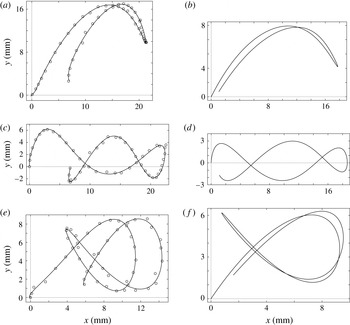
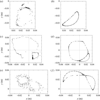
The Lagrangian particle tracking was implemented for several conditions that correspond to different Lissajous vortices. Figure 8 shows the paths that the tracer described in one period for different combinations of frequency and phase shifts of the electromagnetic forcing. Experimental data are represented by circles (
 $\odot$
) joined with a continuous line (to guide the eye) obtained from a polynomial fitting. Since convective effects are not negligible, all paths are open. Although the tracking was performed for only one period, some interesting knotted paths are observed. Limitations of the experimental equipment prevented the observation of web-like trajectories, which require higher frequencies, because, as the frequency is increased, the fluid velocity is reduced and the tracer displacement may become as small as the size of the tracer. Moreover, at high frequencies, the coupling of forcing currents is difficult to implement. In general, numerical results display a very good qualitative agreement with the experimental trajectories. Quantitative agreement is not achieved since numerical calculations assume an ideal advective particle, whereas the tracer used in the experiments is far from being a passive particle. Differences between experimental and numerical values confirm that the real tracer affects somehow the velocity of the surrounding fluid. Anyway, the results indicate that the quasi-two-dimensional model is able to reproduce the main physical features of the electromagnetically driven Lissajous vortices in the shallow layer.
Paths of one tracer during
 $1T$
for different Lissajous vortices: (a,c,e) experimental observations; (b,d,f) numerical calculations; (a,b)
 $f_{x}=20$
mHz,
 $f_{y}=10$
mHz,
 $\unicode[STIX]{x1D719}=0$
,
 $R_{\unicode[STIX]{x1D714}}=240$
; (c,d)
 $f_{x}=30$
mHz,
 $f_{y}=10$
mHz,
 $\unicode[STIX]{x1D719}=\unicode[STIX]{x03C0}/2$
,
 $R_{\unicode[STIX]{x1D714}}=320$
; and (e,f)
 $f_{x}=30$
mHz,
 $f_{y}=20$
mHz,
 $\unicode[STIX]{x1D719}=0$
,
 $R_{\unicode[STIX]{x1D714}}=400$
. For all cases,
 $Re=30$
.

Time maps of a Lissajous vortex obtained with a single particle for
 $200T$
, for
 $f_{x}=10$
mHz,
 $f_{y}=10$
mHz,
 $\unicode[STIX]{x1D719}=\unicode[STIX]{x03C0}/2$
,
 $Re=30$
and
 $R_{\unicode[STIX]{x1D714}}=160$
: (a,c,e) experimental observations; (b,d,f) quasi-two-dimensional numerical calculation; (a,b) tracer released at position (
 $x=0.0097$
,
 $y=-0.0328$
); (c,d) tracer released at (
 $x=0.00973$
,
 $y=0.0281$
); and (e,f) tracer released at (
 $x=-0.0340$
,
 $y=0.0234$
).

The acquisition of experimental data for the construction of the full time map is a very complicated task since, as mentioned before, our experimental method can only photograph a single particle. Nevertheless, a partial time map was obtained by releasing a tracer at a particular initial position and photographing it every period during 200 periods. Figure 9 shows the time map obtained for three different initial positions of the tracer. The experimental conditions corresponds to
 $f_{x}=10$
mHz,
 $f_{y}=10$
mHz,
 $\unicode[STIX]{x1D719}=\unicode[STIX]{x03C0}/2$
,
 $Re=30$
and
 $R_{\unicode[STIX]{x1D714}}=160$
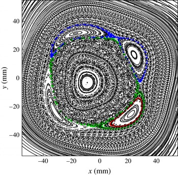
. Figure 9(a,c,e) displays the experimental section while figure 9(b,d,f) shows the section calculated with the numerical model. It is observed that the experimental clustering of points bears the same geometrical properties as the numerically calculated time maps. Specifically, the point distribution found in the experiment that suggests regions containing elliptic points and positions of hyperbolic points are consistent with the numerical calculations. Figure 10 shows the full time map calculated numerically with the parameter values used in the experiment. The sections shown in figure 9, corresponding to the three explored initial positions of the tracer can be observed in red, green and blue colors.
Time map for
 $200T$
due to Lissajous vortex, for
 $f_{x}=10$
mHz,
 $f_{y}=10$
mHz,
 $\unicode[STIX]{x1D719}=\unicode[STIX]{x03C0}/2$
,
 $Re=30$
and
 $R_{\unicode[STIX]{x1D714}}=160$
. Quasi-two-dimensional numerical calculation.

5 Concluding remarks
The laminar flows generated in a thin electrolyte layer by orthogonal localized Lorentz forces have been studied with theoretical and experimental tools. Forces were produced by the interaction of a localized dipolar magnetic field and two imposed alternating electric currents perpendicular to each other. The analysis was focused on exploring the Lagrangian trajectories for small and moderate Reynolds numbers. Assuming that the magnetic field is produced by a point dipole, an approximate two-dimensional analytical solution was obtained for the creeping flow regime. In this case, Lagrangian trajectories were integrated explicitly. In addition, a quasi-two-dimensional numerical model that considers a finite size magnetic dipole was implemented to explore the flow behaviour when inertial effects increase. For small Reynolds numbers, analytical and numerical results agree qualitatively, showing that the action of orthogonal forces originate Lagrangian trajectories that resemble Lissajous figures, preserving the property that rational ratios of the forcing frequencies lead to closed paths while irrational ratios originate non-closed paths that eventually fill the available area. This behaviour changes drastically as inertial effects become relevant, since even for rational frequency ratios Lagrangian paths are no longer closed. Analysis of the evolution of the Lagrangian trajectories with time maps as
 $Re$
increases indicates that the system has a chaotic behaviour similar to that found in area-preserving Hamiltonians.
The flows explored numerically were experimentally observed using a shallow layer of electrolyte. The fluid motion was recorded with particle image velocimetry and the Lagrangian trajectories were observed with particle tracking techniques. The geometrical properties of the numerical and experimental Lagrangian orbits were in qualitative agreement. Particle tracking allowed us to determine time maps of the Lagrangian orbits, and we found similar geometric properties of the distributions of experimental and numerical points. In fact, experimental observations are consistent with the interpretation of the motion of passive tracers advected in a two-dimensional flow as a Hamiltonian system. An interesting case to be explored in future experiments is the use of irrational forcing frequency ratios combined with non-negligible inertial effects. Given the chaotic behaviour displayed even for rather small Reynolds numbers, electromagnetically driven Lissajous vortices could be a mixing strategy that is worth exploring.
Acknowledgements
This research was supported by CONACYT, Mexico, under project 240785. A.F. thanks the Cátedras program from CONACYT.