Effect of fluid inertial torque on the rotational and orientational dynamics of tiny spheroidal particles in turbulent channel flow

Zhiwen Cui; Jingran Qiu; Xinyu Jiang; Lihao Zhao

doi:10.1017/jfm.2023.942

Effect of fluid inertial torque on the rotational and orientational dynamics of tiny spheroidal particles in turbulent channel flow

Published online by Cambridge University Press: 14 December 2023

and

Zhiwen Cui: Affiliation:
AML, Department of Engineering Mechanics, Tsinghua University, 100084 Beijing, PR China
Jingran Qiu: Affiliation:
AML, Department of Engineering Mechanics, Tsinghua University, 100084 Beijing, PR China
Xinyu Jiang: Affiliation:
AML, Department of Engineering Mechanics, Tsinghua University, 100084 Beijing, PR China
Lihao Zhao*: Affiliation:
AML, Department of Engineering Mechanics, Tsinghua University, 100084 Beijing, PR China
*: †Email address for correspondence: zhaolihao@tsinghua.edu.cn

Article contents

Abstract
Introduction
Methodology
Results and discussion
Concluding remarks
Funding
Declaration of interests
References

Rights & Permissions

Abstract

Rotation and orientation of non-spherical particles in a fluid flow depend on the hydrodynamic torque they experience. However, little is known about the effect of the fluid inertial torque on the dynamics of tiny inertial spheroids in turbulent channel flows, as only Jeffery torque has been considered in previous studies by point-particle direct numerical simulations. In this study, we investigate the rotation and orientation of tiny spheroids with both fluid inertial torque and Jeffery torque in a turbulent channel flow. By comparing with the case in the absence of fluid inertial torque, we find that the rotational and orientational dynamics of spheroids is significantly affected by the fluid inertial torque when the Stokes number, which is non-dimensionalized by fluid viscous time scale, is larger than the critical value $St_c\approx 2$, indicating that the fluid inertial torque is non-negligible for most particle cases considered in earlier studies. In contrast to the earlier findings considering only Jeffery torque (Challabotla et al., J. Fluid Mech., vol. 776, 2015, p. R2), we find that prolate (oblate) spheroids with a large Stokes number tend to tumble (spin) in the streamwise–wall-normal plane in a thinner region near the wall due to the presence of the fluid inertial torque. Approaching the channel centre, the flow shear gradually vanishes, but the velocity difference between local fluid and particles is still pronounced and increasing as particle inertia grows. As a result, in the core region, fluid inertial torque is dominant and drives the particles to align with its broad side normal to the streamwise direction rather than a random orientation observed in earlier studies without fluid inertial torque. Meanwhile, the presence of fluid inertial torque enhances the tumbling rates of spheroids in the core region. In addition, the effect of fluid inertial force on the dynamics of spheroids is also examined in this study, but the results indicate the effect of fluid inertial force is weak. Our findings imply the importance of fluid inertial torque in modelling the dynamics of inertial non-spherical particles in turbulent channel flows.

JFM classification

Multiphase and Particle-laden Flows: Particle/fluid flow

Information

Type: JFM Papers
Information: Journal of Fluid Mechanics , Volume 977 , 25 December 2023, A20
DOI: https://doi.org/10.1017/jfm.2023.942 [Opens in a new window]
Copyright: © The Author(s), 2023. Published by Cambridge University Press

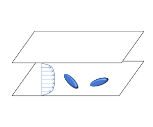
1. Introduction

Non-spherical particle-laden turbulent flows are ubiquitous in both natural and industrial processes, such as pollen transmission (Sabban & van Hout Reference Sabban and van Hout2011), papermaking processes (Lundell, Söderberg & Alfredsson Reference Lundell, Söderberg and Alfredsson2011), biomass combustion (Cui & Grace Reference Cui and Grace2007) and drug delivery industries (Kleinstreuer & Feng Reference Kleinstreuer and Feng2013), to name a few. In practical applications, the particles’ shape has a significant effect on their orientation and rotation, thereby shaping the dynamics of particles and the particle–fluid interactions. Moreover, the presence of the wall makes turbulent flows inhomogeneous and anisotropic as well as results in a strong shear rate in the near-wall region. To conveniently investigate the complicated particle behaviours, the non-spherical particles were normally modelled by spheroids with an axisymmetric shape in earlier theoretical and numerical studies (Voth & Soldati Reference Voth and Soldati2017).

1.1. Angular dynamics of spheroidal particles in turbulent channel flow

Turbulent channel flow (TCF) is a prototype of typical wall-bounded turbulence. Since the pioneering work of Zhang et al. (Reference Zhang, Ahmadi, Fan and McLaughlin2001), numerous numerical studies of non-spherical particles in TCF have been conducted in the past decades via point-particle (PP) (Zhang et al. Reference Zhang, Ahmadi, Fan and McLaughlin2001; Mortensen et al. Reference Mortensen, Andersson, Gillissen and Boersma2008a,Reference Mortensen, Andersson, Gillissen and Boersmab; Marchioli, Fantoni & Soldati Reference Marchioli, Fantoni and Soldati2010; Marchioli & Soldati Reference Marchioli and Soldati2013; Zhao, Marchioli & Andersson Reference Zhao, Marchioli and Andersson2014; Challabotla, Zhao & Andersson Reference Challabotla, Zhao and Andersson2015a; Zhao et al. Reference Zhao, Challabotla, Andersson and Variano2015; Challabotla, Zhao & Andersson Reference Challabotla, Zhao and Andersson2016a; Marchioli, Zhao & Andersson Reference Marchioli, Zhao and Andersson2016; Yuan et al. Reference Yuan, Andersson, Zhao, Challabotla and Deng2017; Ouchene et al. Reference Ouchene, Polanco, Vinkovic and Simoëns2018; Yuan et al. Reference Yuan, Zhao, Andersson and Deng2018a,Reference Yuan, Zhao, Challabotla, Andersson and Dengb; Yang, Zhao & Andersson Reference Yang, Zhao and Andersson2020; Michel & Arcen Reference Michel and Arcen2021, Reference Michel and Arcen2023) and particle-resolved (PR) direct numerical simulations (DNSs) (Uhlmann Reference Uhlmann2008; Do-Quang et al. Reference Do-Quang, Amberg, Brethouwer and Johansson2014; Ardekani et al. Reference Ardekani, Costa, Breugem, Picano and Brandt2017; Eshghinejadfard, Zhao & Thévenin Reference Eshghinejadfard, Zhao and Thévenin2018; Eshghinejadfard, Hosseini & Thévenin Reference Eshghinejadfard, Hosseini and Thévenin2019; Assen et al. Reference Assen, Ng, Will, Stevens, Lohse and Verzicco2022). In PP-DNS, the hydrodynamic forces and torques acting on the particles are modelled analytically or empirically to simulate the motion of particles smaller than the Kolmogorov scale. As for the PR-DNS, the particle–fluid interactions are fully resolved without any models, with the size of the particles generally ten times larger than the Kolmogorov scale to reduce the cost of computations.

In the earlier studies using PP-DNS with a particle Reynolds number $Re_p$ less than one, the hydrodynamic force and torque models are typically obtained under the Stokes flow approximation, which neglects fluid inertial effects. Here, the particle Reynolds number is defined by $Re_p=\tilde {r} |\boldsymbol {u}_s|/\nu$, where $\tilde {r}$ is the volume equivalent radius, $\boldsymbol {u}_s$ is the slip velocity between the fluid and particle velocities and $\nu$ is the fluid kinematic viscosity. Meanwhile, the particle Reynolds number $Re_p$ is proportional to the magnitude of the slip velocity, which increases as particle inertia grows. For $Re_p\ll 1$, the models include the Stokes resistance (Brenner Reference Brenner1963, Reference Brenner1964; Brenner & Cox Reference Brenner and Cox1963) and Jeffery torque (Jeffery Reference Jeffery1922) for non-spherical particles. In the PP-DNSs without considering the effect of gravity, the weak inertial or inertialess prolate spheroids near the wall tend to align their symmetry axes with the streamwise direction, while the weak inertial or inertialess oblate spheroids preferentially align their symmetry axes with the wall-normal direction (Marchioli et al. Reference Marchioli, Fantoni and Soldati2010; Challabotla, Zhao & Andersson Reference Challabotla, Zhao and Andersson2015b; Zhao et al. Reference Zhao, Challabotla, Andersson and Variano2015; Zhao & Andersson Reference Zhao and Andersson2016; Jie et al. Reference Jie, Zhao, Xu and Andersson2019b; Cui et al. Reference Cui, Dubey, Zhao and Mehlig2020b, Reference Cui, Huang, Xu, Andersson and Zhao2021). As the particle inertia increases, prolate spheroids have a tendency to tumble, while oblate spheroids preferentially spin in the streamwise–wall-normal plane near the wall (Marchioli et al. Reference Marchioli, Fantoni and Soldati2010; Marchioli & Soldati Reference Marchioli and Soldati2013; Challabotla et al. Reference Challabotla, Zhao and Andersson2015a; Zhao et al. Reference Zhao, Challabotla, Andersson and Variano2015, Reference Zhao, Challabotla, Andersson and Variano2019). However, in the core region of channel flow, the orientation and rotation of particles are nearly isotropic, irrespective of particle inertia, because of the quasi-isotropy of the turbulence (Marchioli et al. Reference Marchioli, Fantoni and Soldati2010; Marchioli & Soldati Reference Marchioli and Soldati2013; Andersson, Zhao & Variano Reference Andersson, Zhao and Variano2015; Zhao et al. Reference Zhao, Challabotla, Andersson and Variano2015, Reference Zhao, Challabotla, Andersson and Variano2019). In the case of $Re_p\gg 1$, a series of studies by PR-DNS (Do-Quang et al. Reference Do-Quang, Amberg, Brethouwer and Johansson2014; Ardekani et al. Reference Ardekani, Costa, Breugem, Picano and Brandt2017; Eshghinejadfard, Hosseini & Thévenin Reference Eshghinejadfard, Hosseini and Thévenin2017; Eshghinejadfard et al. Reference Eshghinejadfard, Zhao and Thévenin2018, Reference Eshghinejadfard, Hosseini and Thévenin2019) or PP-DNS with empirical models (van Wachem et al. Reference van Wachem, Zastawny, Zhao and Mallouppas2015; Njobuenwu & Fairweather Reference Njobuenwu and Fairweather2016) have reported that long rod-like fibres are slightly normal to the streamwise direction rather than quasi-isotropic distribution in the centre of the channel due to the effect of fluid inertia. When the gravity effect is taken into consideration, there are several studies on the dynamics of spheroidal particles in vertical TCF (Challabotla et al. Reference Challabotla, Zhao and Andersson2016a; Challabotla, Zhao & Andersson Reference Challabotla, Zhao and Andersson2016b; Yuan et al. Reference Yuan, Andersson, Zhao, Challabotla and Deng2017, Reference Yuan, Zhao, Challabotla, Andersson and Deng2018b). Their results show that gravity has significant effects on the patterns of aggregations of inertial spheroids as well as the transport of spheroids along the wall-normal direction, while gravity has a weak influence on the particles’ angular dynamics. Nevertheless, Arcen et al. (Reference Arcen, Ouchene, Khalij and Tanière2017) reported that the symmetry axes of prolate spheroids tend to align to the gravity direction when considering the pitching torque, as obtained by Ouchene et al. (Reference Ouchene, Khalij, Arcen and Tanière2016).

1.2. Importance of fluid inertial torque

The fluid inertial effect on the particle dynamics has recently received growing attention. There are some analytical studies using low-Reynolds-number approximations (Brenner Reference Brenner1961; Dabade, Marath & Subramanian Reference Dabade, Marath and Subramanian2015, Reference Dabade, Marath and Subramanian2016; Einarsson et al. Reference Einarsson, Candelier, Lundell, Angilella and Mehlig2015; Candelier, Mehlig & Magnaudet Reference Candelier, Mehlig and Magnaudet2019; Magnaudet & Abbas Reference Magnaudet and Abbas2021; Candelier et al. Reference Candelier, Qiu, Zhao, Voth and Mehlig2022, Reference Candelier, Mehaddi, Mehlig and Magnaudet2023) as well as numerical and experimental studies at moderate Reynolds numbers (Zastawny et al. Reference Zastawny, Mallouppas, Zhao and van Wachem2012; Ouchene et al. Reference Ouchene, Khalij, Arcen and Tanière2016; Sanjeevi, Kuipers & Padding Reference Sanjeevi, Kuipers and Padding2018; Fröhlich, Meinke & Schröder Reference Fröhlich, Meinke and Schröder2020; Pierson, Kharrouba & Magnaudet Reference Pierson, Kharrouba and Magnaudet2021) aimed at obtaining the fluid inertial hydrodynamic forces and torques. However, to the best of authors’ knowledge, for tiny spheroidal particles suspended in TCF with particle Reynolds number $Re_p\ll 1$, the fluid inertial effects on the hydrodynamic force and torque are not considered in earlier PP-DNSs. When considering the fluid inertial effect, Brenner (Reference Brenner1961) derived the resistance of spheroidal particles moving in flows under the Oseen approximation, which includes the $Re_p$ leading-order fluid inertial force. Dabade et al. (Reference Dabade, Marath and Subramanian2015) derived the fluid inertial torque on spheroidal particles in a uniform flow. Besides, other studies on fluid inertial models of tiny spheroidal particles have been conducted, including a shear-induced torque (Einarsson et al. Reference Einarsson, Candelier, Lundell, Angilella and Mehlig2015; Dabade et al. Reference Dabade, Marath and Subramanian2016) and force (Harper & Chang Reference Harper and Chang1968; Candelier et al. Reference Candelier, Mehlig and Magnaudet2019; Cui et al. Reference Cui, Ravnik, Verhnjak, Hriberšek and Steinmann2019, Reference Cui, Ravnik, Hriberšek and Steinmann2020a) as well as a high-order correction to the fluid inertial force (Candelier et al. Reference Candelier, Mehaddi, Mehlig and Magnaudet2023). For spheroidal particles, recent studies reveal the importance of the fluid inertial torque on the orientation of tiny spheroids settling in homogeneous isotropic turbulence (HIT), even though $Re_p\ll 1$ (Gustavsson et al. Reference Gustavsson, Sheikh, Lopez, Naso, Pumir and Mehlig2019; Anand, Ray & Subramanian Reference Anand, Ray and Subramanian2020; Sheikh et al. Reference Sheikh, Gustavsson, Lopez, Lévêque, Mehlig, Pumir and Naso2020). According to the model of the fluid inertial torque derived by Dabade et al. (Reference Dabade, Marath and Subramanian2015), the shape function and slip velocity between particle and fluid are two significant factors. In addition to the shape function, which just depends on the aspect ratio of the particles, the magnitude and direction of the slip velocity are of importance for the fluid inertial torque. In the sedimentation of spheroidal particles in HIT, the slip velocity mainly induced by gravity is approximately equal to the settling velocity. When the settling velocity is sufficiently large, the effect of the fluid inertial torque surpasses the effect of the Jeffery torque (Jeffery Reference Jeffery1922), making the broad sides of the particles face the gravity direction (Gustavsson et al. Reference Gustavsson, Sheikh, Lopez, Naso, Pumir and Mehlig2019; Anand et al. Reference Anand, Ray and Subramanian2020; Sheikh et al. Reference Sheikh, Gustavsson, Lopez, Lévêque, Mehlig, Pumir and Naso2020). This is qualitatively different from the results in the absence of a fluid inertial torque, where the spheroids tend to align their long axes with the gravity direction (Siewert et al. Reference Siewert, Kunnen, Meinke and Schröder2014; Gustavsson et al. Reference Gustavsson, Jucha, Naso, Lévêque, Pumir and Mehlig2017).

The gravity effect on particles with certain parameters can be significant in HIT, leading to a notable slip velocity caused by the gravity-induced settling velocity (Gustavsson et al. Reference Gustavsson, Sheikh, Lopez, Naso, Pumir and Mehlig2019; Anand et al. Reference Anand, Ray and Subramanian2020; Sheikh et al. Reference Sheikh, Gustavsson, Lopez, Lévêque, Mehlig, Pumir and Naso2020). In TCF, the mechanisms for pronounced slip velocities are intricate, and gravity is not the sole factor to induce a large slip velocity. In the earlier studies on spheroids in TCF without gravity, particles with large particle inertia have pronounced slip velocities relative to the fluid velocity in the buffer layer and core region, where the slip velocity is enhanced as particle inertia increases (Zhao et al. Reference Zhao, Marchioli and Andersson2014; Michel & Arcen Reference Michel and Arcen2021). This pronounced slip velocity is mainly induced by the intense turbulent fluctuations near the wall (Marchioli & Soldati Reference Marchioli and Soldati2002; Zhao et al. Reference Zhao, Marchioli and Andersson2014). Because of the presence of slip velocities induced by the particle–fluid interactions in TCF, the fluid inertial torque can be non-negligible, even though gravity is absent. To understand the effect of the fluid inertial torque induced by the particle inertia in TCF, we ignore gravity intentionally to focus on particle–fluid interactions. Although in some applications, such as in the nuclear (Molyneaux et al. Reference Molyneaux, Harris, Sharkh, Hill and Graaff2017) and lithography (Hyman et al. Reference Hyman, Ballantyne, Friedman, Reilly, Southworth and Dym1982) industries, the particle-to-fluid density ratio is extremely large, the gravity effect can be neglected if the particle Froude number is much larger than one (Sardina et al. Reference Sardina, Schlatter, Picano, Casciola, Brandt and Henningson2012; Milici & De Marchis Reference Milici and De Marchis2016).

1.3. Validity of fluid inertial torque in turbulent channel flow

So far, little is known about the effect of fluid inertial torque on the dynamics of inertial spheroids in TCF. In TCF, there is a strong shear and a relatively large particle slip velocity in the streamwise direction (Zhao et al. Reference Zhao, Marchioli and Andersson2014), suggesting that both the fluid inertial torque and Jeffery torque may both be essential. However, according to Gustavsson et al. (Reference Gustavsson, Sheikh, Lopez, Naso, Pumir and Mehlig2019) and Sheikh et al. (Reference Sheikh, Gustavsson, Lopez, Lévêque, Mehlig, Pumir and Naso2020), the model of fluid inertial torque derived by Dabade et al. (Reference Dabade, Marath and Subramanian2015) is valid in uniform flows, where the shear is absent. While, in a shear flow, the shear-induced fluid inertial effect could be crucial. To estimate the importance of shear-induced fluid inertia relative to the slip-velocity-induced fluid inertia, we can compare the Saffman length scale $l_s=1/\sqrt {Re_s}$ with the Oseen length scale $l_o=1/Re_p$ (Candelier et al. Reference Candelier, Mehlig and Magnaudet2019; Sheikh et al. Reference Sheikh, Gustavsson, Lopez, Lévêque, Mehlig, Pumir and Naso2020). Here, $Re_s$ is the shear Reynolds number based on the mean shear rate $s$, i.e. $Re_s=s\tilde {r}^2/\nu$. When the ratio $l_s/l_o\equiv Re_p/\sqrt {Re_s}$ is much greater than one, the fluid inertia induced by the shear can be ignored (Candelier et al. Reference Candelier, Mehlig and Magnaudet2019; Sheikh et al. Reference Sheikh, Gustavsson, Lopez, Lévêque, Mehlig, Pumir and Naso2020). However, this condition is difficult to satisfy near the wall, where a strong shear is present. In TCF, the ratio of $l_s$ to $l_o$ is simplified to $|u_s|/\sqrt {s\nu }$. By using the friction velocity $u_\tau$ and viscous time scale $t_\nu =\nu /u_\tau ^2$ to non-dimensionalize $u_s$ and $s$, i.e. $|u_s |=|u_s^+ | u_\tau$ and $s=s^+/t_\nu$, we obtain $|u_s|/\sqrt {s\nu }\equiv |u_s^+|/\sqrt {s^+}$. Here, ‘+’ represents the variable is normalized by viscous units. In general, the mean slip velocity $|u_s^+|$ depends on the particle Stokes number and the distance to the wall, and $|u_s^+|$ is usually quite small in the viscous sublayer (Zhao et al. Reference Zhao, Marchioli and Andersson2014). Meanwhile, $s^+$ is approximately equal to unity at the wall, suggesting that the ratio $l_s/l_o$ is close to $|u_s^+|$ in the vicinity of the wall. In the viscous sublayer, the shear Reynolds number satisfies $Re_p\ll \sqrt {Re_s}\ll 1$, i.e. $l_s \ll l_o$, which is out of the range of validity for assuming the dominance of the fluid inertial torque. This means that the effect of shear-induced fluid inertia should be considered. Recently, Candelier et al. (Reference Candelier, Mehlig and Magnaudet2019) conducted an analytical study of the forces and torques acting on a spheroid particle with a small slip velocity under the condition $Re_p\ll \sqrt {Re_s}\ll 1$. Their results indicate that, for spheroidal particles with $Re_p\ll \sqrt {Re_s}\ll 1$, in addition to the Stokes drag force and Jeffery torque, only a $\sqrt {Re_s}$ leading-order shear-induced fluid inertial force needs to be considered but the $\sqrt {Re_s}$ leading-order shear-induced fluid inertial torque vanishes because of the axisymmetric shape. As for the $Re_s$-order shear-induced torque derived by Einarsson et al. (Reference Einarsson, Candelier, Lundell, Angilella and Mehlig2015) and Dabade et al. (Reference Dabade, Marath and Subramanian2016), it should be considered when $Re_p\ll Re_s \ll 1$. In TCF, the ratio $Re_p/Re_s$ is equivalent to $|u_s|/(s\tilde {r})\equiv |u_s^+|/(s^+\tilde {r}^+)$. In the viscous sublayer, $Re_p/Re_s$ is close to $|u_s^+|/\tilde {r}^+$, which is much larger than $Re_p/\sqrt {Re_s}$ when $\tilde {r}^+\ll 1$. This indicates that the region dominated by the $Re_s$-order shear-induced torque is confined to an extremely small region near the wall. Meanwhile, the strong shear mainly exists in the viscous sublayer. Hence, the $Re_s$-order shear-induced fluid inertial torque is negligible compared with the Jeffery torque induced by the strong shear. To support this viewpoint, we conducted a series of PR-DNSs by the immersed boundary method (IBM) to fully resolve spheroid rotation in a shear flow, as shown in Appendix A. As for the $\sqrt {Re_s}$ leading-order shear-induced fluid inertial force (Harper & Chang Reference Harper and Chang1968; Cui et al. Reference Cui, Ravnik, Verhnjak, Hriberšek and Steinmann2019, Reference Cui, Ravnik, Hriberšek and Steinmann2020a), it may affect the translation of particles near the wall. We do not consider this force in the present study to make a direct comparison with the earlier studies, which only considered a Stokesian hydrodynamic force and torque. Therefore, in this study, we adopt fluid inertial torque derived by Dabade et al. (Reference Dabade, Marath and Subramanian2015) and fluid inertial force derived by Brenner (Reference Brenner1961).

The aim of this study is to highlight the importance of fluid inertial torque to tiny inertial spheroidal particles in TCF. Meanwhile, when the fluid inertial torque is non-negligible and how this torque affects the spheroid dynamics in TCF will be addressed in this paper. The remainder of this paper is organized as follows. In § 2, we describe the dynamics of the particles, fluid inertial model and governing equations of the fluid as well as the parameters of the simulations. In § 3, the numerical simulation results of particles are shown and discussed. Finally, in § 4, we summarize the main findings and draw conclusions.

2. Methodology

2.1. Kinematics of particles

In this study, we consider spheroidal particles and their symmetry axes are defined as the particles’ orientation, denoted as $\boldsymbol {n}$ (see figure 1a,b). The shape of the particles is parameterized by the aspect ratio $\lambda$ of the axisymmetry axis to the equatorial axis. Prolate spheroids have $\lambda >1$ while oblate spheroids have $0<\lambda <1$. For spherical particles, $\lambda =1$. To describe the translational and rotational motion of particles, we use the Eulerian frame ($\boldsymbol {x},\boldsymbol {y},\boldsymbol {z}$) and particle frame ($\boldsymbol {x}', \boldsymbol {y}', \boldsymbol {z}'$), as depicted in figure 2, where $({\cdot })^\prime$ represents a quantity in the particle frame. Furthermore, we use unit quaternions $\boldsymbol {E} =[e_0,e_1,e_2,e_3]^{\rm T}=[\cos ({\varPsi }/{2}),b_1\sin ({\varPsi }/{2}),b_2\sin ({\varPsi }/{2}),b_3\sin ({\varPsi }/{2})]^{\rm T}$ that an arbitrary rotation transformation can be obtained through rotating about an axis $\boldsymbol {b}=[b_1,b_2,b_3]$ with an angle $\varPsi$ from the original orientation. The schematic of the rotation transformation of a spheroid is shown in figure 1(c). We use an orthogonal tensor $\boldsymbol{\mathsf{Q}}$ to describe the rotation, whose relationship with quaternions is

(2.1)

\begin{equation} \boldsymbol{\mathsf{Q}}=\left[\begin{matrix} {e_{0}^{2}+e_{1}^{2}-e_{2}^{2}-e_{3}^{2}} & {2\left(e_{1} e_{2}-e_{0} e_{3}\right)} & {2\left(e_{1} e_{3}+e_{0} e_{2}\right)} \\ {2\left(e_{1} e_{2}+e_{0} e_{3}\right)} & {e_{0}^{2}-e_{1}^{2}+e_{2}^{2}-e_{3}^{2}} & {2\left(e_{2} e_{3}-e_{0} e_{1}\right)} \\ {2\left(e_{1} e_{3}-e_{0} e_{2}\right)} & {2\left(e_{2} e_{3}+e_{0} e_{1}\right)} & {e_{0}^{2}-e_{1}^{2}-e_{2}^{2}+e_{3}^{2}} \end{matrix}\right]. \end{equation}

A first-order tensor, i.e. vector $\boldsymbol {p}$, depicted in the Eulerian frame can be transformed from the particle frame via $\boldsymbol {p}=\boldsymbol{\mathsf{Q}} \boldsymbol {\cdot }\boldsymbol {p}'$, while a second-order tensor $\boldsymbol{\mathsf{B}}$ in the Eulerian frame can be transformed from the particle frame via $\boldsymbol{\mathsf{B}}=\boldsymbol{\mathsf{Q}} \boldsymbol {\cdot } \boldsymbol{\mathsf{B}}' \boldsymbol {\cdot } \boldsymbol{\mathsf{Q}}^{\rm T}$. The governing equation of $\boldsymbol {E}$ is

(2.2)

\begin{equation} \frac{\mathrm{d}{\boldsymbol{E}}}{\mathrm{d}t}=\frac{1}{2}\boldsymbol{\mathsf{G}}^{\rm T} \boldsymbol{\cdot} \boldsymbol{ \omega}', \end{equation}

where

(2.3)

\begin{equation} \boldsymbol{\mathsf{G}}=\left[\begin{matrix} -e_1 & e_0 & -e_3 & e_2\\ -e_2 & -e_3 & e_0 & e_1\\ -e_3 & e_2 & -e_1 & e_0\\ \end{matrix}\right], \end{equation}

and $\boldsymbol { \omega }'$ is the particle angular velocity depicted in the particle frame.

Figure 1.

Schematic of the directions of (a) prolate and (b) oblate spheroids. (c) The rotation transformation of a spheroid from its original orientation.

Figure 2.

Schematic of the Eulerian frame $(\boldsymbol {x},\boldsymbol {y},\boldsymbol {z})$ and the particle frame $(\boldsymbol {x}',\boldsymbol {y}',\boldsymbol {z}')$ in TCF.

2.2. Dynamics of particles

The governing equation of a spheroidal particle's translational motion is (Brenner Reference Brenner1961; Brenner & Cox Reference Brenner and Cox1963)

(2.4)

\begin{equation} m_p\frac{\mathrm{d}{\boldsymbol{v}}}{\mathrm{d}t}= \mu \tilde{r}\left(\boldsymbol{\mathsf{K}}_{s}+\frac{Re_p}{32{\rm \pi}}\boldsymbol{\mathsf{K}}_I\right)\boldsymbol{\cdot} (\boldsymbol{u}-\boldsymbol{v}), \end{equation}

where $\boldsymbol {u}$ represents the fluid velocity at the particle location, $\mu$ is the viscosity of the fluid, $\boldsymbol {v}$ is the particle velocity, $m_p$ is the mass of the particle, $\tilde {r}$ is the volume equivalent radius of the particle, $Re_p$ is the Reynolds number of the particle $\tilde {r}|\boldsymbol {u}-\boldsymbol {v}|/\nu$ ($\nu$ is the kinematic viscosity of the fluid), $\boldsymbol{\mathsf{K}}_s$ is the dimensionless Stokes resistance tensor and $\boldsymbol{\mathsf{K}}_I$ is the dimensionless resistance tensor contributed by fluid inertia. According to Brenner (Reference Brenner1961), $\boldsymbol{\mathsf{K}}_I$ is expressed by

(2.5)

\begin{equation} \boldsymbol{\mathsf{K}}_I=3\boldsymbol{\mathsf{K}}_s \boldsymbol{\cdot}\boldsymbol{\mathsf{K}}_s-(\boldsymbol{\mathsf{K}}_s: \hat{\boldsymbol{u}}_s \hat{\boldsymbol{u}}_s)\boldsymbol{\mathsf{K}}_s,\quad \hat{\boldsymbol{u}}_s=(\boldsymbol{u}-\boldsymbol{v})/|\boldsymbol{u}-\boldsymbol{v}|. \end{equation}

Here, $\boldsymbol {\hat {u}}_s$ is the direction of the slip velocity. The Stokes resistant coefficients for arbitrary spheroids in the particle frame are (Brenner Reference Brenner1963)

(2.6a–c)

\begin{equation} {K_s'}_{,xx} =\frac{16{\rm \pi}}{\chi+\alpha},\quad {K_s'}_{,yy} =\frac{16{\rm \pi} }{\chi+\beta},\quad {K_s'}_{,zz} =\frac{16{\rm \pi} }{\chi+\lambda^2\gamma}. \end{equation}

Here, the dimensionless shape factors $\alpha,\beta, \gamma$ and $\chi$ are expressed as follows:

(2.7)

\begin{equation} \left.\begin{gathered} \alpha=\int_{0}^{\infty} \frac{{\rm d} \xi}{\Delta(\xi)(1+\xi)},\quad \beta=\int_{0}^{\infty} \frac{{\rm d} \xi}{\Delta(\xi)(1+\xi)},\quad \gamma=\int_{0}^{\infty} \frac{{\rm d} \xi}{\Delta(\xi)(\lambda^2+\xi)},\\ \chi=\int_{0}^{\infty} \frac{{\rm d} \xi}{\Delta(\xi)},\quad\text{where } \Delta(\xi)=(1+\xi)\sqrt{\lambda^2+\xi}. \end{gathered}\right\} \end{equation}

The analytical expressions of the shape factors are listed in table 1. Note that $\boldsymbol{\mathsf{K}}_s$ and $\boldsymbol{\mathsf{K}}_I$ are both anisotropic tensors and dependent on the particle orientation relative to the slip velocity. Generally, the effect of the particle's inertia is measured by the ratio of the particle's response time to the fluid time scale, denoted as the Stokes number $St$. Here, the fluid time scale is the fluid viscous time scale of channel flow, i.e. $t_\nu =\nu /u_\tau ^2$, where $u_\tau$ is the wall friction velocity. Unlike a sphere, the response time of a spheroidal particle strongly depends on its orientation relative to the slip velocity with the fluid. The particle response time is estimated by assuming that particle orientation is randomly distributed (Shapiro & Goldenberg Reference Shapiro and Goldenberg1993). The particle's response time $\tau _p$ thereby is

(2.8)

\begin{equation} \tau_p=\left\{\begin{array}{@{}ll} \dfrac{D a^2 \lambda}{9\nu} \dfrac{2\ln (\lambda+\sqrt{\lambda^2-1})}{\sqrt{\lambda^2-1}}, & \lambda>1;\\ \dfrac{D a^2 \lambda}{9\nu} \dfrac{{\rm \pi}-2\arctan \dfrac{\lambda}{\sqrt{1-\lambda^2}}}{\sqrt{1-\lambda^2}}, & 0 <\lambda<1, \end{array}\right. \end{equation}

where $D$ is the particle-to-fluid density ratio and $a$ is the semi-length of the equatorial axis. In this work, only the translational response time is adopted to describe the particle inertia (Zhao et al. Reference Zhao, Challabotla, Andersson and Variano2015).

Table 1.

Shape factors of particles, where $A=2\ln (\lambda +\sqrt {\lambda ^2-1})$ and $B=2\arctan ({\lambda }/{\sqrt {1-\lambda ^2}})$.

In addition to the translational dynamics of a spheroid, the particle angular dynamics is a vital part of the present study. The angular dynamics of the spheroids is described by the Euler equation, i.e.

(2.9)

\begin{equation} \boldsymbol{\mathsf{I}}'\boldsymbol{\cdot} \frac{\mathrm{d}{\boldsymbol{ \omega}'}}{\mathrm{d}t}+\boldsymbol{ \omega}'\times (\boldsymbol{\mathsf{I}}'\boldsymbol{\cdot} \boldsymbol{ \omega}')=\boldsymbol{T}', \end{equation}

where $\boldsymbol{\mathsf{I}}'$ is the inertial moment tensor, $\boldsymbol { \omega }'$ is the angular velocity and $\boldsymbol {T}'$ is the principal torque acting on the spheroid. The angular dynamics of the particles is solved in the particle frame (see figure 2), in which the moments of inertia of the spheroid are constant about the principal axes (Challabotla et al. Reference Challabotla, Zhao and Andersson2015a). Furthermore, the particle spatial orientations are calculated through (2.2). Besides, the total torque $\boldsymbol {T}'$ is the sum of the Jeffery torque (Jeffery Reference Jeffery1922), $\boldsymbol {T}_J'$, and of the contribution from the fluid inertia, $\boldsymbol {T}_I'$, i.e.

(2.10)

\begin{equation} \boldsymbol{T}'=\boldsymbol{T}_J'+\boldsymbol{T}_I'. \end{equation}

As for spheroids, the Jeffery torque is (Jeffery Reference Jeffery1922)

(2.11)

\begin{equation} \left.\begin{gathered} {T_J'}_{x} =\frac{16{\rm \pi}\mu a^3 }{3(\beta+\lambda^2 \gamma)} \left[(1-\lambda^2)S_{yz}'+(1+\lambda^2)(\varOmega_x'-\omega_x')\right],\\ {T_J'}_{y} =\frac{16{\rm \pi}\mu a^3}{3(\alpha+\lambda^2 \gamma)} \left[(\lambda^2-1)S_{xz}'+(\lambda^2+1)(\varOmega_y'-\omega_y')\right],\\ {T_J'}_{z} =\frac{32{\rm \pi}\mu a^3}{3(\alpha+ \beta)}(\varOmega_z'-\omega_z'). \end{gathered}\right\} \end{equation}

The fluid inertial torque in the Eulerian frame is expressed as (Dabade et al. Reference Dabade, Marath and Subramanian2015)

(2.12)

\begin{equation} \boldsymbol{T}_I=-\rho_f |\boldsymbol{u}_s|^2 \tilde{a}^3F_\lambda \left(\frac{\boldsymbol{u}_s}{ |\boldsymbol{u}_s|}\boldsymbol{\cdot} \boldsymbol{n} \right) \left(\frac{\boldsymbol{u}_s}{ |\boldsymbol{u}_s|}\times \boldsymbol{n}\right), \end{equation}

where

(2.13)

\begin{equation} \tilde{a}=\left\{\begin{array}{@{}lc} \lambda a & ,\lambda>1;\\ a & ,\lambda<1,\\ \end{array}\right. \end{equation}

and $F_\lambda$ is a shape function that depends on the particle's shape (Dabade et al. Reference Dabade, Marath and Subramanian2015). To compute conveniently, the final form of the fluid inertial torque in the particle frame $\boldsymbol {T}_I'$ is

(2.14)

\begin{equation} \boldsymbol{T}_I'=-\rho_f \tilde{a}^3F_\lambda {u_{s}'}_{3}\left(\begin{matrix} {u_{s}'}_{2}\\ -{u_{s}'}_{1}\\ 0 \end{matrix}\right). \end{equation}

In addition, the forms of the shape function $F_\lambda$ for prolate and oblate spheroids are different. For the prolate spheroids ($\lambda >1$), the eccentricity of the spheroid $e=\sqrt {1-\lambda ^{-2}}$ and the corresponding shape function $F_\lambda$ is expressed as

(2.15)

\begin{align} F_\lambda &= \frac{-{\rm \pi} e^2(420e+2240e^3+4249e^5-2152e^7)}{315((e^2+1)\tanh^{-1}e-e)^2((1-3e^2)\tanh^{-1}e-e)} \nonumber\\ &\quad +\frac{{\rm \pi} e^2(420+3360e^2+1890e^4-1470e^6)\tanh^{-1}e}{315((e^2+1)\tanh^{-1}e-e)^2((1-3e^2)\tanh^{-1}e-e)} \nonumber\\ &\quad -\frac{{\rm \pi} e^2(1260e-1995e^3+2730e^5-1995e^7)(\tanh^{-1}e)^2}{315((e^2+1)\tanh^{-1}e-e)^2((1-3e^2)\tanh^{-1}e-e)}. \end{align}

For the oblate spheroids ($0<\lambda <1$), the eccentricity of the spheroid is $e=\sqrt {1-\lambda ^2}$ and the corresponding shape function is

(2.16)

\begin{align} F_\lambda &=\frac{{\rm \pi} e^3(-420+3500e^2-9989e^4+4757e^6)}{315(-e\sqrt{1-e^2}+(1+2e^2)\arcsin e)(e\sqrt{1-e^2}+(2e^2-1)\arcsin e)^2} \nonumber\\ &\quad +\frac{210{\rm \pi} e^2(2-24e^2+69e^4-67e^6+20e^8)\arcsin e}{315\sqrt{1-e^2}(-e\sqrt{1-e^2}+(1+2e^2)\arcsin e)(e\sqrt{1-e^2}+(2e^2-1)\arcsin e)^2} \nonumber\\ &\quad +\frac{105{\rm \pi} e^3(12-17e^2+24e^4)(\arcsin e)^2}{315(-e\sqrt{1-e^2}+(1+2e^2)\arcsin e)(e\sqrt{1-e^2}+(2e^2-1)\arcsin e)^2}. \end{align}

Figure 3 shows the shape function varying with aspect ratio $\lambda$. According to (2.14), the shape function reflects the strength of the torque. Figure 3 shows that the strength of the fluid inertial torque on oblate spheroids monotonically increases as the eccentricity increases (the corresponding aspect ratio decreases). The corresponding $F_\lambda$ reaches $\lim _{\lambda \rightarrow 0}F_\lambda =\frac {38}{9}-{17\,216}/{945 {\rm \pi}^2}\approx 2.38$ when $\lambda \rightarrow 0$ and the corresponding eccentricity reaches one, while the strength of the inertial torque on prolate spheroids reaches a peak at $\lambda \approx 1.88$ and $F_\lambda \approx -0.96$. In addition, it is clear that the torque strength of oblate spheroids is larger than that of prolate spheroids with the same eccentricity $e$ according to figure 3.

Figure 3.

Function $F_\lambda$ vs the aspect ratio $\lambda$ of spheroids. The red lines represent $\lambda =0.02$, 0.1, 0.33, 1, 3, 10 and 50 from left to right, respectively. The inset shows function $F_\lambda$ vs the eccentricity $e$.

Nevertheless, the model of the fluid inertial torque (Dabade et al. Reference Dabade, Marath and Subramanian2015) is deduced in a uniform flow in the absence of shear. The validation of this model performed by Jiang et al. (Reference Jiang, Zhao, Andersson, Gustavsson, Pumir and Mehlig2021) is also in a uniform flow with the fixed inclination angle of the spheroid relative to the flow. However, the flow near the wall has a strong shear, and it is a concern whether the model of the fluid inertial torque is still valid in a strong shear flow. To qualitatively verify the analytical expression of fluid inertial torque in a shear flow, an assessment is performed by simulating a single particle freely rotating in a linear shear flow by the IBM in Appendix A. The results show that the fluid inertial torque model also works in a flow with strong shear.

2.3. Direct numerical simulations of fluid and particles

In the current study, we performed DNSs of spheroidal particles in a TCF by using the Eulerian–Lagrangian method. The carrier fluid is computed in the Eulerian frame, the flow is incompressible and isothermal and is governed by the Navier–Stokes equation and continuity equation as follows:

(2.17a)

$$\begin{gather} \frac{\partial \boldsymbol{u}}{\partial t}+(\boldsymbol{u} \boldsymbol{\cdot} \boldsymbol{ \nabla}) \boldsymbol{u} =-\frac{\boldsymbol{ \nabla} p}{\rho_f}+\nu \nabla^2 \boldsymbol{u}, \end{gather}$$

(2.17b)

$$\begin{gather}\boldsymbol{ \nabla} \boldsymbol{\cdot} \boldsymbol{u}=0. \end{gather}$$

Here, $\boldsymbol {u}$ is the fluid velocity, $p$ is the pressure, $\rho _f$ is the density of the fluid and $\nu$ is the kinematic viscosity of the fluid. We set $\hat {\boldsymbol {x}}$, $\hat {\boldsymbol {y}}$ and $\hat {\boldsymbol {z}}$ as the streamwise, wall-normal and spanwise directions, respectively. The domain size is $4{\rm \pi} h \times 2h \times 2{\rm \pi} h$ and the corresponding mesh size is $192 \times 128 \times 192$, where $h$ is the half-height of the channel. Periodic boundary conditions are applied in the spanwise and streamwise directions, while no-slip boundary conditions are applied at both walls. A pseudo-spectral method is used in the streamwise ($\hat {\boldsymbol {x}}$) and the spanwise ($\hat {\boldsymbol {z}}$) directions and second-order finite-difference discretization is used in the wall-normal direction ($\kern0.7pt \hat {\boldsymbol {y}}$). The Reynolds number $Re_b$ based on the bulk velocity of fluid $U_b$, i.e. $Re_b=U_bh/\nu$, is 2820, while the corresponding frictional Reynolds number $Re_\tau$ based on the friction velocity on the wall $u_\tau$, i.e. $Re_\tau =u_\tau h/\nu$, is 180. Here, the friction velocity on the wall is defined by $u_\tau =\sqrt {\tau _w/\rho _f}$, where $\tau _w$ is the wall shear stress. In two homogeneous directions, i.e. $\hat {\boldsymbol {x}}$ and $\hat {\boldsymbol {z}}$, the meshes are uniform with $\Delta x^+=11.78$ and $\Delta z^+=5.89$. For the wall-normal direction, the mesh is stretched by a hyperbolic tangent function with the stretching factor $sk=1.5$. The size of mesh near the wall is $\Delta y_{min}^+\sim 0.8$. The time integration is achieved by means of an explicit second-order Adams–Bashforth scheme, and the time step $\Delta t^+=0.068$. In the present fully developed TCF, there are several distinct regions divided in the wall-normal direction such as the viscous sublayer ($y^+<5$), buffer layer ($5< y^+<30$), logarithm layer ($y^+>30$, $y/h<0.3$), core region ($y^+>50$) and near-wall region ($y^+<50$) (Pope Reference Pope2000). In this study, the near-wall region includes the viscous sublayer, buffer layer and part of the logarithm layer, where the viscous contribution to the shear stress is significant (Pope Reference Pope2000).

For the particles, the motions are governed by (2.4) and (2.9). A second-order Lagrangian interpolation is utilized to obtain the local fluid velocity and velocity gradient tensor at the particle's location from the neighbouring grids. The time-integrated scheme for the particle is the same as the fluid integration. The particle–wall collision is fully elastic, and the rebound is detected by the volume equivalent radius $\tilde {r}=\lambda ^{1/3}a$. Note that only the wall-normal particle velocity is reversed and the particle orientation remains the same after a collision. The same computational method has been widely employed in our previous studies (Challabotla et al. Reference Challabotla, Zhao and Andersson2015a; Cui et al. Reference Cui, Dubey, Zhao and Mehlig2020b, Reference Cui, Huang, Xu, Andersson and Zhao2021; Cui & Zhao Reference Cui and Zhao2022; Jie et al. Reference Jie, Cui, Xu and Zhao2022). In this study, we tracked swarms of 300 000 spheroids of each case with the aspect ratio ranging from 0.02 to 50, and Stokes number ranging from 1 to 100. The corresponding values of the shape function $F_\lambda$ are shown in the stem plot in figure 3. Considering that the effect of fluid inertial torque increases as particle inertia grows, it is of interest to explore how spheroids behave with significant particle inertia, which can only be realized by increasing the density ratio with the constraint of small particle size to satisfy the PP assumption. In this study, we change the particle-to-fluid density ratios and fix the volume equivalent radius $\tilde {r}^+\approx 0.15$ for all types of particles to vary the Stokes number as listed in table 2. The particles are split into two groups with different configurations, as depicted in table 3. In group A, the gas is air and the half-height of the channel $h=2$ cm, where the particle-to-fluid density ratio is $O(10^3)$. In group B, the particles have very large particle-to-fluid density ratio with $\lambda =50$ and $\lambda =0.02$ at $St=30$ as well as for all aspect ratios at $St=100$, as depicted in table 2. These large particle-to-fluid density ratios in group B can be found in some realistic applications, such as the nuclear (Molyneaux et al. Reference Molyneaux, Harris, Sharkh, Hill and Graaff2017) and lithography (Hyman et al. Reference Hyman, Ballantyne, Friedman, Reilly, Southworth and Dym1982) industries, where helium is one of the important protected gases. Therefore, in group B, we set the gas as helium and the corresponding half-height is $h=5$ cm.

Table 2.

Density ratio of particles. Note that the volume equivalent radius for all particles is $\tilde {r}^+\approx 0.15$.

Table 3.

Different flow configurations of groups A and B (air and helium).

Meanwhile, the size of the particles with different aspect ratios is shown in table 4. For the most elongated particle with $\lambda =50$, the maximum length $l^+$ in wall units is around 4 and with a corresponding diameter in wall units of the cross-section $d^+$ around 0.08. In this study, the Kolmogorov length scale $\eta ^+$ ranges from 1.54 at the wall to 3.68 at the centre of the channel. Therefore, the ratio $l^+/\eta ^+$ of the prolate spheroids with $\lambda =50$ is from 1.106 to 2.644. Ravnik, Marchioli & Soldati (Reference Ravnik, Marchioli and Soldati2018) proposed an empirical formula to evaluate the calculation error of the Jeffery torque with large aspect ratios in a TCF, i.e. $\textrm {Err}\approx 0.041 St ^{-0.34}(l^+/\eta ^+)^{1.44}$, where $l^+/\eta ^+<8$. According to this formula, for the case with $\lambda =50$, we have $4\,\%$–$16\,\%$ error at $St=1$, $2.7\,\%$–$9.4\,\%$ error at $St=5$, $1.5\,\%$–$5\,\%$ error at $St=30$ and $1\,\%$–$3.4\,\%$ error at $St=100$, indicating that the error decreases as the Stokes number increases. Besides, the effect of the fluid inertial torque becomes more significant as the Stokes number increases. The errors of the Jeffery torque for the current settings are acceptable for making a meaningful comparison with the fluid inertial torque.

Table 4.

Parameters of particle size. Here, the Kolmogorov length scale $\eta ^+$ ranges from 1.54 (close to the wall) to 3.68 (at the centre of the channel).

The gravity effect is normally ignored when the particle Froude number $Fr_p=U_b/(g\tau _p)=Re_\tau ^2Re_b \nu ^2/(St gh^3)$, i.e. the ratio between the Stokes drag and gravity, is larger than one (Sardina et al. Reference Sardina, Schlatter, Picano, Casciola, Brandt and Henningson2012; Milici et al. Reference Milici, De Marchis, Sardina and Napoli2014), indicating that particles are mainly driven by the flows rather than the gravity. Here, $g$ is the gravitational acceleration, $\tau _p$ is the response time of the particles and $St$ is the Stokes number based on the viscous time scale of the fluid $t_\nu$. Accordingly, $g\tau _p$ represents the settling velocity of a particle, while $U_b$ is the characteristic velocity of particle translation due to $|\boldsymbol {u}-\boldsymbol {v} |\sim U_b$. The particle Froude numbers in the present study are much larger than one, as shown in table 5, indicating that the effect of gravity is negligible.

Table 5.

Froude number of particles $Fr_p$ for different Stokes numbers.

Specifically, to explore the effect of fluid inertia, we consider three cases with different particle models, as shown table 6. In the case S-J, the force and torque acting on the spheroids are both within the Stokes flow regime, where the fluid inertial effects are neglected, i.e. $\boldsymbol{\mathsf{K}}_I=\boldsymbol{\mathsf{0}}$ and $\boldsymbol {T}_I=\boldsymbol {0}$. In the case S-JI, only the additional fluid inertial torque is considered, and the fluid inertial force is still neglected, i.e. $\boldsymbol{\mathsf{K}}_I =\boldsymbol{\mathsf{0}}$, compared with the case S-J. The additional fluid inertial force and torque are both considered in the case SI-JI. In the earlier studies, the PP-DNSs of spheroidal particles were performed without any fluid inertial models (Zhang et al. Reference Zhang, Ahmadi, Fan and McLaughlin2001; Marchioli et al. Reference Marchioli, Fantoni and Soldati2010, Reference Marchioli, Zhao and Andersson2016; Marchioli & Soldati Reference Marchioli and Soldati2013; Zhao & van Wachem Reference Zhao and van Wachem2013; Zhao et al. Reference Zhao, Marchioli and Andersson2014, Reference Zhao, Challabotla, Andersson and Variano2015; Challabotla et al. Reference Challabotla, Zhao and Andersson2015a). Therefore, the case S-J is included as a reference. The cases S-JI and SI-JI are used to illustrate the effects of fluid inertial torque. The comparison between the cases S-JI and SI-JI explains the effect of the fluid inertial force.

Table 6.

The particle models for different cases.

In this study, the number of particles of each case is around 300 000. The corresponding volume fraction of each case is approximately $4\times 10^{-6}$ and the maximum mass loading is 0.27, indicating that the feedback of particles onto the fluid phase is weak (Zhou et al. Reference Zhou, Zhao, Huang and Xu2020), which justifies the one-way coupling approach adopted in the present study (Elgobashi Reference Elgobashi2006). The statistics are obtained within a time window from $t^+=6800$ to $10\,200$, where $t^+=0$ represents the time when particles are initially injected into the fully developed TCFs. Meanwhile, in this time window, the orientation and rotation of spheroidal particles have reached a statistically steady state to ensure reliable statistics (Marchioli et al. Reference Marchioli, Fantoni and Soldati2010; Zhao et al. Reference Zhao, Marchioli and Andersson2014; Challabotla et al. Reference Challabotla, Zhao and Andersson2015a).

3. Results and discussion

3.1. Particle Reynolds numbers

At first, we examine the particle Reynolds number in the whole channel. In figure 4, the particle Reynolds number $Re_p$ for all cases is below 0.5, which guarantees that our simulation satisfies the condition $Re_p\ll 1$. Meanwhile, according to the results in figure 4, it is obvious that $Re_p$ increases as the Stokes number increases. In this study, $Re_p$ is defined as $\tilde {r}|\boldsymbol {u}-\boldsymbol {v}|/\nu$, where $\tilde {r}$ is the volume equivalent radius and is set as 0.15 viscous scales for all particle types. Therefore, the statistics of $Re_p$ are calculated directly through the averaged difference $|\boldsymbol {u}-\boldsymbol {v}|$, multiplying by a constant $\tilde {r}$. Note that the averaged difference $|\boldsymbol {u}-\boldsymbol {v}|$ refers to the norm of the slip velocity. It means that figure 4 also reflects the slip velocity with different models of the hydrodynamics or aspect ratios of the particles. As shown in figure 4, the regions with the large slip velocity are primarily located in the buffer layer, while the regions with the smallest slip velocity are in the vicinity of the wall. Meanwhile, the largest discrepancies in the results for different cases with large Stokes numbers are observed in the buffer layer. The differences in the norm of the slip velocity between the particles with different aspect ratios in the case S-J are quite small, but become obvious in cases S-JI and SI-JI, particularly in the case SI-JI. These discrepancies increase as the Stokes number grows. More importantly, this reflects that the fluid inertial resistance can significantly impact the slip velocity.

Figure 4.

The Reynolds number of a particle $Re_p$ based on the volume equivalent radius, i.e. $\tilde {r}=a\lambda ^{1/3}$, with different Stokes numbers and particle models for whether considering fluid inertia or not. The Stokes numbers from (a) to (d) are 1, 5, 30 and 100, respectively. Symbols, dashed lines and solid lines represent the results for S-J, S-JI and SI-JI, respectively.

3.2. Tumbling and spinning rates of spheroids

In this section, we explore how the fluid inertial torque affects particle rotation. In general, there are two distinct rotation modes for spheroids, i.e. tumbling and spinning. Here, the tumbling motion represents spheroid rotation about a non-symmetry axis, and the spinning motion represents spheroid rotation about the symmetry axis. Note that the tumbling and spinning rates of spheroids are independent of the frame. In the particle frame, the tumbling and spinning rates are computed by ${\omega '_x}^2+{\omega '_y}^2$ and $\omega _z'\omega '_z$, respectively, where the prime indicates that the variables are depicted in the particle frame and the $z'$-axis is the symmetry axis in the present study. In a Eulerian frame, the tumbling rate is $\dot {n_i}\dot {n_i}=\omega _i \omega _i-\omega _in_i\omega _jn_j$, while the spinning rate is expressed as $\omega _in_i\omega _jn_j$. Therefore, the tumbling and spinning rates can be obtained either in the particle frame or Eulerian frame. In the present numerical solver (Zhao et al. Reference Zhao, Challabotla, Andersson and Variano2015; Jie et al. Reference Jie, Xu, Dawson, Andersson and Zhao2019a), the particle angular dynamics is solved in the particle frame and therefore it is more convenient for us to compute tumbling and spinning rates in the particle frame. To further explore the effect of fluid inertial torque on particle rotation in wall turbulence, we discuss prolate and oblate spheroids separately.

3.2.1. Prolate spheroids: $\lambda >1$

Figure 5 shows the tumbling rates of prolate spheroids with $y^+$. When the Stokes number is small ($St=1$), the tumbling rates of the prolate spheroids are similar to the inertialess prolate spheroids reported in Challabotla et al. (Reference Challabotla, Zhao and Andersson2015b). Therefore, we observe that the tumbling rates of the prolate spheroids with large aspect ratios are lower than those of the spherical particles near the wall. That is because the strong shear rate near the wall makes their symmetry axes align with the streamwise direction. Meanwhile, at small Stokes number, where fluid inertia and particle inertia are both weak, the discrepancies in the results for different models are quite small. As the Stokes number increases, the tumbling rate of the prolate spheroids increases and becomes even larger than the tumbling rate of spherical particles near the wall. This is because prolate spheroids tend to rotate about the axis with the maximum particle inertial moment in the strong shear plane, i.e. tumbling in the shear plane for prolate spheroids. Away from the wall, the tumbling rates of prolate spheroids are smaller than those of spherical spheroids. Nevertheless, when comparing the results of the three different cases, namely cases S-J, S-JI and SI-JI, as particle inertia increases, the tumbling rates of the cases S-JI and SI-JI are larger than those of case S-J in the core region, but smaller in the near-wall region. This reflects the significant effect of fluid inertial torque on spheroid rotation throughout the channel. Moreover, the effect of fluid inertial torque is against with the effect of particle inertia and increases as particle inertia grows, as shown in Appendix A. These differences induced by fluid inertial torque become obvious as the Stokes number increases.

Figure 5.

Tumbling rates of prolate spheroids with (a) $St=1$, (b) $St=5$, (c) $St=30$ and (d) $St=100$. Symbols, dashed lines and solid lines represent the results for S-J, S-JI and SI-JI, respectively.

As for the spinning rates, as shown in figure 6, with increasing Stokes number, the spinning rates of prolate spheroids decrease and fall below the spinning rates of spherical ones near the wall, but their spinning rates are larger than those of spheres close to the centre of the channel. These observations are contrary to the trend observed for tumbling rates. Nevertheless, compared with the results of case S-J, the spinning rates of cases S-JI and SI-JI are larger near the wall. However, in the core region, there are no discrepancies of the results of the different cases with different models, reflecting that the fluid inertial effect on the spinning rates of prolate spheroids is weak in the core region. According to the results in the near-wall region, as depicted in figures 5 and 6, we conclude that the fluid inertial torque could attenuate the tumbling rate but enhance the spinning rate of prolate spheroids because the torque could make prolate spheroids rotate away from the shear plane, i.e. the $x{-}y$ plane in this study. Another possible explanation is that the presence of the fluid inertial torque may weaken the effect of particle inertia, which corresponds to a decreasing local Stokes number of rotation. However, in the core region, fluid inertial torque mainly enhances the tumbling rates of prolate spheroids but has little influence on the spinning rates of prolate spheroids. Obviously, there are two distinct mechanisms of the effect of fluid inertial torque on prolate spheroid rotations. In the near-wall region, the strong shear rate dominates the rotations of prolate spheroids, and the variations of the orientation distributions of prolate spheroids with respect to the velocity gradients influenced by the fluid inertial torque attenuate the tumbling rate but enhance the spinning rates. Far away from the wall, i.e. near the channel centre, the fluid inertial torque directly contributes to the rotation about the asymmetry axis of the spheroid, resulting in strengthened tumbling rates.

Figure 6.

Spinning rates of prolate spheroids with (a) $St=1$, (b) $St=5$, (c) $St=30$ and (d) $St=100$. Symbols, dashed lines and solid lines represent the results for S-J, S-JI and SI-JI, respectively.

3.2.2. Oblate spheroids: $0<\lambda <1$

As for the oblate spheroids, depicted in figures 7 and 8, the spinning rotation is dominant near the wall. That is because the moment of inertia of oblate spheroids reaches the maximum when the particle rotates about its symmetry axis. However, in the core region, the tumbling rotation pattern of oblate spheroids is predominant compared with the sphere. In the strong shear flow, the fluid inertial torque can make oblate spheroids depart from the spinning mode and enhance their tumbling rates in strong shear flow, which has been demonstrated by the simulations of oblate spheroids rotating in a simple shear flow, as depicted in Appendix A. This implies that the orientation of oblate spheroids relative to the strong shear plane near the wall has a significant effect on the rotation of oblate spheroids, which is similar to prolate spheroids. According to figure 7(b) for $St=5$, in the range of $y^+=2\sim 10$, the tumbling rates of oblate spheroids in cases S-JI and SI-JI with $\lambda =0.33$ and $0.1$ are slightly stronger compared with the results of case S-J, while there are no prominent differences in other regions. This means that the tumbling mode of oblate spheroids is sensitive to the particle inertia because the maximum norm of the slip velocity appears in this region. As $St$ increases to 30 and 100, the range of $y^+$ with the enhanced tumbling rates of oblate spheroids in cases S-JI and SI-JI are extended from the wall to the core region, as depicted in figure 7(c,d). The possible explanation is that fluid inertial torque mainly contributes to the rotation about the asymmetry axis of a spheroid, which increases the tumbling rate. This trend becomes more and more prominent as the Stokes number increases. With regard to the spinning rate of the oblate spheroids, at $St=1$, there are no differences in the results for the three cases. As the Stokes number increases, the effect of fluid inertial torque becomes non-negligible in the near-wall region, which attenuates the spinning rate of the oblate spheroids obviously compared with the case S-J. However, close to the centre of the channel, the discrepancies of the spinning rate of the oblate spheroids between different cases are quite small. This indicates that fluid inertial torques mainly affect the tumbling rates of oblate spheroids in channel flow. Similar to prolate spheroid, the reduction of the spinning rate of the oblate ones corresponds to the increase of the tumbling rate near the wall. Meanwhile, as the effect of the fluid inertial torque increases, the effect of the particle inertia of oblate spheroids decreases.

Figure 7.

Tumbling rates of oblate spheroids with (a) $St=1$, (b) $St=5$, (c) $St=30$ and (d) $St=100$. Symbols, dashed lines and solid lines represent the results for S-J, S-JI and SI-JI, respectively.

Figure 8.

Spinning rates of oblate spheroids with (a) $St=1$, (b) $St=5$, (c) $St=30$ and (d) $St=100$. Symbols, dashed lines and solid lines represent the results for S-J, S-JI and SI-JI, respectively.

3.3. Orientations of spheroids

Compared with spherical particles, the orientational dynamics of spheroidal particles is more complicated. According to (2.9), the orientation of particles is affected not only by the physical properties of the particles, e.g. aspect ratio and density, but also by the surrounding fluid field, such as the fluid velocity and fluid-velocity gradients. In the earlier studies, only the Stokes resistance and torque are taken into account (Marchioli et al. Reference Marchioli, Fantoni and Soldati2010, Reference Marchioli, Zhao and Andersson2016; Marchioli & Soldati Reference Marchioli and Soldati2013; Challabotla et al. Reference Challabotla, Zhao and Andersson2015a). Therefore, in the vicinity of the wall, prolate spheroids tumble but oblate spheroids tend to spin like a wheel in the streamwise–wall-normal plane. In the centre of the channel, the orientations are approximately random due to the quasi-isotropic turbulence. These distinctive rotations and orientation patterns are associated with the different characteristics of the flow in the different regions in the channel, such as the strong mean shear rate near the wall and the quasi-isotropic flow near the centre (Zhao et al. Reference Zhao, Challabotla, Andersson and Variano2015). However, the role of fluid inertial torque at small particle Reynolds numbers in wall turbulence has received little attention to date. It is unclear how the distribution of the particle orientation or rotation is affected by the fluid inertial torque in wall turbulence. According to the aforementioned analysis conducted on the slip velocity of particles in the TCF, the slip velocities of particles are large in the buffer layer and channel centre, where the effect of the fluid inertial torque is significant. Unlike the anisotropic orientations of settling particles in HIT, in which gravity causes a large slip velocity (Gustavsson et al. Reference Gustavsson, Sheikh, Lopez, Naso, Pumir and Mehlig2019; Sheikh et al. Reference Sheikh, Gustavsson, Lopez, Lévêque, Mehlig, Pumir and Naso2020), the settling velocity of the gravity effect is neglected in the current study. Instead, the large slip velocity is induced by the turbulent structures in wall turbulence. According to the study of the inertial torque (Gustavsson et al. Reference Gustavsson, Sheikh, Lopez, Naso, Pumir and Mehlig2019; Anand et al. Reference Anand, Ray and Subramanian2020; Sheikh et al. Reference Sheikh, Gustavsson, Lopez, Lévêque, Mehlig, Pumir and Naso2020), the angular dynamics of spheroids in wall turbulence could also be changed by the fluid inertial torque due to the prominent slip velocity. To better understand these effects on the orientations of particles, we discuss the results of prolate and oblate spheroids separately in the following sections.

3.3.1. Prolate spheroids: $\lambda >1$

Figure 9 shows the correlations of particle orientation relative to the streamwise, wall-normal and spanwise directions, denoted as $\langle |\cos \theta _i|\rangle$($i=x,y,z$). Note that $\langle |\cos \theta _i|\rangle =0.5$ represents an isotropic distribution of orientation. For the Stokes number $St=1$, the statistics of particle orientation are nearly independent of the models used in the different cases (see figure 9a–c). The reason is that the slip velocity is too small to induce any significant effects of the fluid inertial torque and fluid inertial resistance. At this small Stokes number $St=1$, prolate spheroids tend to align with the streamwise direction in the near-wall region as the aspect ratio $\lambda$ increases. Moreover, these preferential alignments with streamwise direction slightly decrease in the viscous sublayer. Meanwhile, as the aspect ratio $\lambda$ increases, the orientations of prolate spheroids tend to distribute in the $x-z$ plane with the position close to the wall. As the Stokes number increases to 5, as shown in figure 9(d–f), the results of cases S-JI and SI-JI, in which the fluid inertial torque is taken into account, exhibit slight differences from case S-J primarily in the buffer layer. But there is no discrepancy of the results between cases S-JI and SI-JI, reflecting a negligible effect of fluid inertial resistance. Away from the wall, the results show no discrepancy for the different models. For this Stokes number $St=5$, it is prominent that fluid inertial torque enhances the tendency of prolate spheroids with high aspect ratio to align to the streamwise direction in the buffer layer, except for the spheroids with $\lambda =3$. When the Stokes number further increases to $St=30$ and $100$, the discrepancies between the case S-J with the case S-JI or SI-JI are enlarged from the buffer layer to the core region, as shown in figure 9(g–l). The orientation patterns of particles change when the fluid inertial torque is considered compared with the case S-J. Nevertheless, this difference is negligible close to the wall. According to the statistics $\langle |\cos \theta _z|\rangle$ in figure 9, as the Stokes number increases near the wall, the orientation of a prolate spheroid tends to be normal to the spanwise direction, indicating that prolate spheroid has a strong tendency to tumble with its symmetry axis rotating in the $x$–$y$ plane. Since the strong shear and vorticity of the fluid are in the $x{-}y$ plane near the wall, the prolate spheroid at large Stokes number exhibits a prominent tumbling rate. However, this strong-tumbling region of prolate spheroid is confined to the wall when the fluid inertial torque is considered. For cases S-JI and SI-JI, the prolate spheroids tend to orient isotopically in the buffer layer, whereas the prolate spheroids exhibit a slight tendency to be normal to the streamwise direction in the core region. Furthermore, the tendency of the prolate spheroid to be normal to the streamwise direction decreases as the aspect ratio increases. This reflects the weaker effect of fluid inertial torque on the extremely slender prolate spheroids than that on the spheroids with moderate aspect ratio. This can be interpreted via the non-monotonic variation of the fluid inertial torque with the aspect ratio of prolate spheroids (see figure 3).

Figure 9.

Orientations of prolate spheroids $\langle |\cos \theta _i|\rangle (i=x,y,z)$ with (a–c) $St=1$, (d–f) $St=5$, (g–i) $St=30$ and (j–l) $St=100$; the three columns of panels from left to right correspond to the $x$, $y$ and $z$ components, respectively. Symbols, dashed lines and solid lines represent the results for S-J, S-JI and SI-JI, respectively.

The alignment of spheroids can be decomposed into $|\cos \theta _i|=\langle |\cos \theta _i|\rangle +|\cos \theta _i|^*$, where $i=x$, $y$ and $z$. Here, $|\cos \theta _i|^* (i=x,y,z)$ are the fluctuations of the alignment of spheroids. The root-mean-squares (RMSs) of the alignment fluctuations of prolate spheroids are depicted in figure 10. For spherical particles, the alignment fluctuations are equal to 0.29. Approaching the core region, the alignment fluctuations for all kinds of spheroids are close to the fluctuations of spherical particles. However, close to the wall, the alignment fluctuations of spheroids vary with shape, Stokes number and fluid inertial model. At low Stokes number, prolate spheroids have preferential alignments near the wall, but we can observe smaller alignment fluctuations in the wall-normal direction, reflecting that prolate spheroids tend to tumble or oscillate in the streamwise–spanwise plane. At large Stokes number, prolate spheroids exhibit smaller alignment fluctuations in the spanwise direction, referring to a strong tumbling in the streamwise–wall-normal plane. When the fluid inertial torque is considered, the alignment fluctuations of cases S-JI and Si-JI in the streamwise and spanwise directions are larger than those of case S-J near the wall. This reflects that the presence of fluid inertial torque weakens spheroid preferential alignments near the wall, which is consistent with the results shown in figure 9.

Figure 10.

Orientation fluctuations of prolate spheroids $|\cos \theta _i|^*_{RMS}(i=x,y,z)$ with (a–c) $St=1$, (d–f) $St=5$, (g–i) $St=30$ and (j–l) $St=100$. The three columns of panels from left to right correspond to the $x$, $y$ and $z$ components, respectively. Symbols, dashed lines and solid lines represent the results for S-J, S-JI and SI-JI, respectively.

To better understand the relationship between particle alignment and slip velocity, we examine the correlations between the directions of the prolate spheroids and the corresponding slip velocity, as shown in figure 11. The correlation $|\cos \phi |$ is defined as

(3.1)

\begin{equation} |\cos\phi|= \frac{|\boldsymbol{n} \boldsymbol{\cdot} (\boldsymbol{u}-\boldsymbol{v})|}{|\boldsymbol{u}- \boldsymbol{v}|}. \end{equation}

Here, $\boldsymbol {n}$ is the orientation vector of a spheroid. At small Stokes number $St=1$, as aspect ratio increases, the tendency of prolate spheroids to align in the direction of slip velocity becomes pronounced in the vicinity of the wall. As the position $y^+$ far away from the wall, the alignments of prolate spheroids with the direction of slip velocity become weaker. As Stokes number increases, $\langle |\cos \phi |\rangle$ becomes smaller than 0.5, reflecting a tendency of particles to align normal to the slip velocity, in the core region when the fluid inertial torque is taken into consideration. This tendency is weak close to the wall because of the predominant viscous torque on the particles, namely the Jeffery torque induced by the near-wall shear rate. According to figures 9 and 11, the small discrepancies observed between cases S-JI and SI-JI are ascribed to the fluid inertial resistance. The presence of fluid inertial resistance increases the resistant coefficient and attenuates the slip velocity, which accordingly reduces the magnitude of the fluid inertial torque.

Figure 11.

The cosine values of the relative angles $\phi$ between symmetry axes of prolate spheroids and directions of slip velocity of particles compared with the local fluid velocity with (a) $St=1$, (b) $St=5$, (c) $St=30$ and (d) $St=100$. Symbols, dashed lines and solid lines represent the results for S-J, S-JI and SI-JI, respectively.

Figure 12 displays the probability density distributions of the correlations between the directions of prolate spheroids and the slip velocity at different positions of the channel. According to figure 12, there are two typical alignment modes. One is the prolate spheroid tending to align in the slip velocity direction. While the other one is that the symmetry axis of a prolate spheroid preferentially orients normal to the slip velocity direction. At different positions and Stokes number, spheroids exhibit different alignment modes. First, for the case S-J, where the fluid inertial torque is absent, there is a pronounced align-to-slip-velocity mode from $St = 1$ to $100$. Near the wall, this mode is diminished as the Stokes number increases, which is attributed to the attenuation of preferential alignment of prolate spheroid by the particle inertia. At $y^+=30$ and $180$, the distribution of the align-to-slip-velocity mode is weakly associated with Stokes number. Second, for the cases S-JI and SI-JI, where the fluid inertial torque is considered, the align-to-slip-velocity mode is still observed at $y^+=3$ and $13$. But, as the Stokes number increases, this preferential alignment becomes less obvious due to the effect of particle inertia. However, at $y^+=30$ and $180$, where the mean shear gradually vanishes, the effect of fluid inertial torque becomes significant and drives the prolate spheroids with large Stokes number ($St=30$ and $100$) to align normal to the slip velocity. These alignment modes of prolate spheroids are consistent with the statistics depicted in figures 9 and 11, reflecting the significance of the fluid inertial torque to spheroid orientation.

Figure 12.

Probability distribution functions of $|\cos \phi |$ of the relative angle between the symmetry axes of prolate spheroids with $\lambda =10$ and directions of slip velocity of particles compared with the local fluid velocity for different Stokes numbers at (a) $y^+=3$, (b) $y^+=13$, (c) $y^+=30$ and (d) $y^+=180$. Symbols, dashed lines and solid lines represent the results for S-J, S-JI and SI-JI, respectively.

3.3.2. Oblate spheroids: $0<\lambda <1$

Compared with the prolate spheroids with the same eccentricity, the preferential orientations of the oblate spheroids are more susceptible to the fluid inertial torque due to the differences in the shape functions for the fluid inertial torque. According to figure 3, the shape function of the oblate spheroid approaches a constant as the aspect ratio $\lambda \rightarrow 0$ or eccentricity $e\rightarrow 1$, while it tends to zero as the aspect ratio $\lambda \rightarrow \infty$ or eccentricity $e\rightarrow 1$ for the prolate spheroid. According to (2.14), the effect of fluid inertial torque on oblate spheroids is enhanced as the aspect ratio decreases to zero. In this study, figure 13 shows the orientations of the symmetry axis of the oblate spheroids in TCF. In figure 13(a–c), where $St=1$, the lines for the different computational cases (S-J, S-JI and SI-JI) coincide, indicating that the influence of the fluid inertial torque is negligible when the Stokes number is small enough. Therefore, oblate spheroids with $St=1$ tend to align in the wall-normal direction near the wall. While approaching the channel centre, the orientation of oblate spheroids gradually becomes isotropic. Note that the baseline of cosine value around 0.5 of spherical particles indicates an isotropic distribution of orientation. As for the case with $St=1$, the particle inertial effect is weak and results in a negligible slip velocity and fluid inertial torque. By increasing the Stokes number to $St=5$ (see figure 13d–f), the obvious differences between the case S-J with the case S-JI or SI-JI are observed in the buffer layer, and more apparent than those of the prolate spheroids in figure 9(d–f), which can be explained by the different particle shape dependence in the shape function of fluid inertial torque (see figure 3). In the buffer layer, the oblate spheroids of the cases S-JI and SI-JI have prominent alignments with the wall-normal direction compared with the results of the case S-J. In the core region, there are no discrepancies for the different models. As the Stokes number continually increases to $St=30$ or $100$, the discrepancies of the oblate spheroids of the cases S-JI and SI-JI relative to the case S-J are enlarged in both the buffer layer and the core region, as shown in figure 13(g–l). At the same time, the oblate spheroids preferentially align to the streamwise directions near the channel centre when the fluid inertial torque is considered (case S-JI or SI-JI), while the symmetry axes of oblate spheroids of the cases S-JI and SI-JI depart from the spanwise direction and the $x$–$y$ plane in the buffer layer compared with the case S-J. In the viscous sublayer, the effect of fluid inertial torque on the particles is quite weak. These indicate that, as the Stokes number increases, the effect of fluid inertial torque is obvious in the buffer layer and then affects the behaviours of spheroids in the core region.

Figure 13.

Orientations of oblate spheroids $\langle |\cos \theta _i|\rangle (i=x,y,z)$ with (a–c) $St=1$, (d–f) $St=5$, (g–i) $St=30$ and (j–l) $St=100$. The three columns of panels from left to right correspond to the $x$, $y$ and $z$ components, respectively. Symbols, dashed lines and solid lines represent the results for S-J, S-JI and SI-JI, respectively.

Akin to the prolate spheroids, the alignment of oblate spheroids can be decomposed to mean orientations and fluctuations. The alignment fluctuations of the oblate spheroids, denoted as $|\cos \theta _i|^*_{RMS} (i=x,y,z)$, are displayed in figure 14. We observe that the alignment fluctuations of oblate spheroids in three different directions are all close to the alignment fluctuations of spherical ones near the channel centre. In the near-wall region, there are pronounced differences of the alignment fluctuations with different shape, Stokes number and fluid inertial model. In the vicinity of the wall, the alignment fluctuations in the streamwise direction are decreasing as the aspect ratio $\lambda$ decreases to 0.02 at low Stokes numbers ($St=1$ and $5$). As the Stokes number increases to $St=100$, the alignment fluctuations along the wall-normal and spanwise directions decrease in the viscous sublayer. It is obvious that the presence of the fluid inertial torque enhances the alignment fluctuations in all three directions with increasing Stokes number in the buffer layer. This implies that fluid inertial torque can further weaken the spinning mode of oblate spheroids in the near-wall region and make the region, where oblate spheroids spin in $x$–$y$ plane, confined to a thinner region close to the wall, compared with the results without fluid inertial torque.

Figure 14.

Orientation fluctuations of oblate spheroids $|\cos \theta _i|^*_{RMS}(i=x,y,z)$ with (a–c) $St=1$, (d–f) $St=5$, (g–i) $St=30$ and (j–l) $St=100$. The three columns of panels from left to right correspond to the $x$, $y$ and $z$ components, respectively. Symbols, dashed lines and solid lines represent the results for S-J, S-JI and SI-JI, respectively.

The statistical relative angle between the orientation of oblate spheroids and the direction of slip velocity is shown in figure 15. Regarding the case S-J, in the buffer layer, oblate spheroids tend to be perpendicular to the slip velocity, while in the core region the alignment of oblate spheroids relative to slip velocity is nearly random. However, for the cases S-JI and SI-JI, as the Stokes number increases, the oblate spheroids tend to align in the direction of slip velocity in the core region. In addition, the tendency of alignment to the slip velocity in case S-JI is more significant than that in case SI-JI. This is due to the inclusion of the additional fluid inertial resistance in case SI-JI, which attenuates the amplitude of the slip velocity and indirectly affects the fluid inertial torque on the particles. Moreover, the preferential alignment normal to the direction of the slip velocity is confined to the vicinity of the wall as the Stokes number increases, indicating that the fluid inertial effect becomes significant as particle inertia grows in near-wall region.

Figure 15.

The cosine values of the relative angles $\phi$ between symmetry axes of oblate spheroids and directions of slip velocity of particles compared with the local fluid velocity with (a) $St=1$, (b) $St=5$, (c) $St=30$ and (d) $St=100$. Symbols, dashed lines and solid lines represent the results for S-J, S-JI and SI-JI, respectively.

To compare the distributions of the oblate alignment of the different cases (S-J, S-JI and SI-JI) at different regions in the channel, we examine the probability density functions of the absolute cosine values of the relative angle between the symmetry axis of the oblate spheroids and the direction of the slip velocity (defined in (3.1)) at $y^+=3,13,30$ and $180$ in figure 16. At $y^+=3$, where the shear rate is strong, the distributions of case S-J (symbols) show that the oblate spheroids tend to be normal to the slip velocity at $St=1$. For the cases with $St = 5$, $30$ and $100$, the alignment distributions shown in figure 16 are bimodal, i.e. there exist align-to-slip-velocity and perpendicular-to-slip-velocity modes simultaneously. In the viscous sublayer of $y^+<5$, the shear is strong and drives the weak inertial ($St=1$) oblate spheroids to align with the wall-normal direction, which is perpendicular to the direction of the slip velocity. With a large $St$, the symmetry axis of oblate spheroids tends to align in the spanwise direction, which is also perpendicular to the slip velocity. However, at an intermediate $St=5$, the effect of particle inertia moves the oblate spheroid orientation away from the wall-normal direction, but the effect of particle inertia is not strong enough to align the oblate spheroid in the spanwise direction. Therefore, we can observe a non-monotonic relationship of the perpendicular-to-slip-velocity mode with Stokes number. Nevertheless, the fluid inertial torque makes the align-to-slip-velocity mode more prominent at large Stokes numbers (see solid and dashed lines). These observations indicate that fluid inertial torque has a significant effect on oblate spheroids, competing with the Jeffery torque near the wall. The results at $y^+=13$ and $30$ show that the oblate spheroids of the case S-J (symbols) tend to align normal to the slip velocity, independent of Stokes number. While the oblate spheroids of the cases S-JI (dashed lines) and SI-JI (solid lines) tend to align perpendicular to the slip velocity with small Stokes numbers ($St=1$ and $5$), but preferentially align to the slip velocity direction with large Stokes numbers ($St=30$ and $100$). In the core region, as shown in figure 16(d) ($y^+=180$), the oblate spheroids of the cases S-JI and SI-JI with $St=30$ and $100$ have preferential alignments with the slip velocity due to the effect of fluid inertial torque.

Figure 16.

Probability distribution functions of $|\cos \phi |$ of relative angle between the symmetry axes of oblate spheroids with $\lambda =0.1$ and directions of slip velocity of particles compared with the local fluid velocity for different Stokes numbers at (a) $y^+=3$, (b) $y^+=13$, (c) $y^+=30$ and (d) $y^+=180$. Symbols, dashed lines and solid lines represent the results for S-J, S-JI and SI-JI, respectively.

3.4. The dimensionless parameter $R$

In the current study, the principal torque acting on particles is obtained by linearly adding the Jeffery torque as well as the fluid inertial torque. The competition between these two torques could affect the rotation behaviours of the particles. To estimate the relative strengths of these two torques, Sheikh et al. (Reference Sheikh, Gustavsson, Lopez, Lévêque, Mehlig, Pumir and Naso2020) defined a dimensionless parameter $R$ to estimate the relative importance of the fluid inertial effects on angular dynamics of particles. The dimensionless parameter $R$ is defined by

(3.2)

\begin{equation} {R}=\frac{\langle|\boldsymbol{u}-\boldsymbol{v}|^2\rangle}{\nu \langle|\boldsymbol{ \varOmega}- \boldsymbol{ \omega}|\rangle}, \end{equation}

where $\boldsymbol {u}$ is the fluid velocity, $\boldsymbol { \varOmega }$ is the angular velocity of the fluid, $\boldsymbol {v}$ is the particle velocity, $\boldsymbol { \omega }$ is the particle angular velocity and $\nu$ is the kinetic viscosity of the fluid.

Sheikh et al. (Reference Sheikh, Gustavsson, Lopez, Lévêque, Mehlig, Pumir and Naso2020) proposed $\langle |\boldsymbol {T}_I|\rangle /\langle |\boldsymbol {T}_J|\rangle \sim {R}$. When ${R} \gg 1$, the fluid inertial torque dominates, and the spheroids tend to align their broad side normal to the slip velocity. If ${R} \ll 1$, the effect of fluid inertial torque is negligible. Besides, in the formula of ${R}$ (see (3.2)), the slip angular velocity of the particle $|\boldsymbol { \varOmega } -\boldsymbol { \omega }|$ has the same order as the local fluid strain $|\boldsymbol{\mathsf{S}}|$. Therefore, ${R}$ can be similar to the ratio ${R}\sim Re_p^2/Re_s$. This indicates that the fluid inertial torque can be ignored when particles Reynolds number $Re_p\ll \sqrt {Re_s}$ but it is crucial when $Re_p\gg \sqrt {Re_s}$. To understand the relative importance of fluid inertial torque and Jeffery torque, figure 17 shows the value of ${R}$ as function of position $y^+$ for different inertia and shape aspect ratios of the particles. At a small Stokes number $St=1$, as shown in figure 17(a), the values of ${R}$ are all below one. It is safe to neglect fluid inertial torque for particles with small inertia according to Sheikh et al. (Reference Sheikh, Gustavsson, Lopez, Lévêque, Mehlig, Pumir and Naso2020). This illustrates why the results of spheroids at $St=1$ have no obvious discrepancies between different cases. Furthermore, figure 17(b–d) reflects that the regions for ${R}$ over one are extended from the centre of the channel to the wall as particle inertia increases. It is obvious that ${R}$ reaches a peak in the buffer layer and logarithm layer, and falls down in the core region as the distance to the wall increases. This is consistent with the results reported in figures 9 and 13. Therefore, we can observe the differences in the results of different cases first appear in the buffer layer with increasing particle inertia. To estimate when the fluid inertial torque is important in TCFs, the relationship between the peak values ${R}$ of each case and particles inertia is shown in figure 18(a). For spheroids with different aspect ratios, the peak values ${R}_{\textit{max}}$ are different. If we use ${R}_{\textit{max}} \approx 1$ as a criterion suggested by Sheikh et al. (Reference Sheikh, Gustavsson, Lopez, Lévêque, Mehlig, Pumir and Naso2020), the corresponding critical Stokes numbers $St_c$ for different particles range from 1.9 to 2.9. Nevertheless, ${R}$ is a relatively rough parameter to quantify the effect of fluid inertial torque. To be convenient, we choose $St_c\approx 2$ as a critical Stokes number to determine whether fluid inertial torque should be considered in the TCF at $Re_\tau \approx 180$. It indicates that ignoring fluid inertial torque in the simulation for $St\lesssim 2$ is safe. When $St \gg 2$, e.g. $St=10$ and $30$, the fluid inertial torque on spheroidal particles cannot be ignored in TCF. To verify this critical number $St_c\approx 2$, we calculate the maximum deviations at different $y^+$ of the tumbling rate $D_{tumble}(y^+)$, spinning rate $D_{spin}(y^+)$ and orientation $D_{orient}(y^+)$ of spheroids between cases S-J and SI-JI, as shown in figure 18(b–d). The formulas of corresponding deviation are defined as

(3.3)

\begin{equation} \left.\begin{gathered} D_{tumble}(y^+)=\widetilde\max|\text{tumbling rate of SI-JI}-\text{tumbling rate of S-J}|, \\ D_{spin}(y^+)=\widetilde\max|\text{spinning rate of SI-JI}-\text{spinning rate of S-J}|,\\ \begin{aligned} D_{orient}(y^+)&=\widetilde\max[(\langle|\cos\theta_x|\rangle_{S\text{-}J}- \langle|\cos\theta_x|\rangle_{SI\text{-}JI})^2\\ &\quad +(\langle|\cos\theta_y|\rangle_\text{S-J}-\langle|\cos\theta_y|\rangle_{SI\text{-}JI})^2\\ &\quad +(\langle|\cos\theta_z|\rangle_\text{S-J}-\langle|\cos\theta_z|\rangle_{SI\text{-}JI})^2]^{1/2}.\end{aligned} \end{gathered}\right\} \end{equation}

Here, $\widetilde {\max }$ represents a function to find the maximum value of the results of spheroids with different aspect ratios. Figure 18(b–d) demonstrates that $St_c\approx 2$ in the current study can clearly distinguish the $St$-region where the fluid inertial torque should be considered or not. However, in the most PP-DNS studies of inertial spheroidal particles in TCF, the Stokes numbers of most particle cases based on the viscous time scale are over $St_c\approx 2$. Therefore, the importance of fluid inertial torque should be emphasized when considering inertial spheroidal particles in wall turbulence. Moreover, note that the critical $St_c\approx 2$ is obtained at $Re_\tau =180$. For the turbulent flows with higher Reynolds numbers, the critical Stokes number could vary with Reynolds number of the fluids. According to the recent studies of inertial spheroids in the TCF with $Re_\tau$ up to 1000 (Michel & Arcen Reference Michel and Arcen2023), the $Re_\tau$-dependence of the statistics of the translation velocities of spheroids is the same as the $Re_\tau$-dependence of the statistics of the fluid velocities. Therefore, the maximum norm of the slip velocity of particles in the buffer layer could slightly increase as $Re_\tau$ grows up. Meanwhile, ${R}\sim Re_p^2/Re_s$, which can be expressed as ${R}\sim |\boldsymbol {u}_s^+|^2/s^+$ in channel flow. The mean shear rate $s^+$ in wall units is nearly independent of $Re_\tau$. Consequently, $\textrm {Re}$ could slightly grow with increasing $Re_\tau$. Therefore, as $Re_\tau$ increases, the corresponding critical Stokes number should be smaller if we still use ${R}\approx 1$ as a criterion. It means that for high-Reynolds-number TCFs, the fluid inertial torque could be important for the orientational dynamics of spheroids even at a smaller Stokes number compared with the results in low-Reynolds-number flows.

Figure 17.

The dimensionless parameter $R$ in the wall-normal direction; (a) $St=1$, (b) $St=5$, (c) $St=30$ and (d) $St=100$. Dashed lines and solid lines represent the results of cases S-JI and SI-JI, respectively.

Figure 18.

(a) Value of $\textrm {Re}$ vs Stokes number $St$. Symbols represent the cases that consider fluid inertia, and the solid line represents function ${R}=0.31 St^{1.38}$. The red pentagram symbol represents the point ${R}\approx 1$ and $St\approx 2.3$. (b–d) The deviations of particle rotations and orientations between the cases S-J and SI-JI, i.e. (b) tumbling rate $D_{tumble}(y^+)$, (c) spinning rate $D_{spin}(y^+)$ and (d) orientation $D_{orient}(y^+)$. Here, the red dashed line represents $St_c\approx 2$.

4. Concluding remarks

This study systematically investigates the effect of fluid inertial torque on the orientation and rotation of tiny inertial spheroids in a TCF via the PP-DNS. In contrast to the earlier studies, where only a Stokesian hydrodynamic force and torque are considered, our findings reveal that the slip-induced fluid inertial torque derived by Dabade et al. (Reference Dabade, Marath and Subramanian2015) significantly affects the rotational and orientational dynamics of particles over a wide range of Stokes numbers. This indicates that the fluid inertial torque is significant when modelling the dynamics of tiny spheroids in wall turbulence. Notably, the region where the fluid inertial torque is non-negligible in almost the entire channel.

In the TCF, the variations of the rotation and orientation of spheroids with $y^+$ are the results of the competitions between fluid inertial torque and Jeffery torque in different layers. In the viscous sublayer, the shear rate is the strongest but the slip velocity is quite small, indicating that the fluid inertial torque is negligible. Therefore, the rotation and orientation of spheroids in this region are the same as the results in the earlier studies without fluid inertial torque. For example, weak inertial prolate (oblate) spheroids tend to align their symmetry axes with the streamwise (wall-normal) direction; large inertial prolate (oblate) spheroids have a tendency to tumble (spin) in the strong gradient–vorticity plane, i.e. streamwise–wall-normal plane. Away from the wall, in the buffer layer, the shear rate and slip velocity are both pronounced. The strong flow shear drives the inertial spheroids to rotate with their longest axis in the streamwise–wall-normal plane, but the presence of the fluid inertial torque hinders this tendency and confines these motions to a thinner region close to the wall. Therefore, in the buffer layer, the fluid inertial torque makes the orientation of spheroids close to an isotropic distribution. Approaching the core region, the flow shear gradually vanishes and the effect of the fluid inertial torque becomes predominant, driving the particle to have its broad side facing the streamwise direction. That is because the pronounced component of the slip velocity is in the streamwise direction, and spheroids tend to align their broad side normal to the slip velocity direction, i.e. the orientation of prolate (oblate) spheroids has a tendency to be perpendicular (parallel) to the slip velocity. Besides, the presence of fluid inertial torque enhances the tumbling rate of spheroids in the core regions.

Moreover, the effect of fluid inertial torque becomes significant as the Stokes number increases. To estimate when the effect of fluid inertial torque is significant, a dimensionless parameter $\textrm {Re}$ is used to reflect the relative importance between fluid inertial torque and the Jeffery torque in wall turbulence (Sheikh et al. Reference Sheikh, Gustavsson, Lopez, Lévêque, Mehlig, Pumir and Naso2020). By analysing the relationship between $\textrm {Re}$ and $St$ as well as the deviations of rotation and orientation between the case SI-JI and case S-J, we propose a critical value $St_c\approx 2$ in the TCF at $Re_\tau =180$. When the Stokes number is much larger than this critical value, the fluid inertial torque has a non-negligible influence on the angular dynamics of inertial spheroids.

Meanwhile, we only consider the fluid inertial torque derived by Dabade et al. (Reference Dabade, Marath and Subramanian2015) and the fluid inertial force derived by Brenner (Reference Brenner1961). Close to the wall, the particle Reynolds number and the shear Reynolds number may satisfy $Re_p\ll \sqrt {Re_s}\ll 1$, where the $\sqrt {Re_s}$-order shear-induced fluid inertial force, such as the Saffman lift force for spheroids (Harper & Chang Reference Harper and Chang1968), may play a significant role in the translational dynamics of particles in the vicinity of the wall. Therefore, a shortcoming of this study is to neglect the shear-induced fluid inertial lift force on spheroids, but this lift force has limited influence on the spheroids far away from the wall. Recently, some improved shear-induced lift models of rods in shear flow were proposed by Cui et al. (Reference Cui, Ravnik, Verhnjak, Hriberšek and Steinmann2019, Reference Cui, Ravnik, Hriberšek and Steinmann2020a), which can be taken into consideration in future studies. Besides, the gravity effect, Reynolds-number effect as well as the effects of the high-order fluid inertial models, such as $Re_s$-order fluid inertial torques (Einarsson et al. Reference Einarsson, Candelier, Lundell, Angilella and Mehlig2015; Dabade et al. Reference Dabade, Marath and Subramanian2016) could be considered in future works. Meanwhile, it is worth noting that the density ratio at $St=100$ is indeed large in the present study and confined to some special applications in reality (Hyman et al. Reference Hyman, Ballantyne, Friedman, Reilly, Southworth and Dym1982; Molyneaux et al. Reference Molyneaux, Harris, Sharkh, Hill and Graaff2017). It is of interest to keep a common density ratio but to change the spheroid size to realize different Stokes numbers in fully resolved simulations in future work, in which the effect of fluid inertia and the particle-size effect can be explored.

Funding

This work was supported by the Natural Science Foundation of China (grant numbers 92252104, 92252204 and 12388101) and the China Postdoctoral Science Foundation (grant number 2022M721849).

Declaration of interests

The authors report no conflict of interest.

Appendix A. Rotation of a spheroidal particle in a linear shear flow

The fluid inertial torque derived by Dabade et al. (Reference Dabade, Marath and Subramanian2015) should satisfy $\sqrt {Re_s}\ll Re_p \ll 1$. However, in the current study, it is difficult to satisfy this condition when the particle is close to the wall, where shear is strong but slip velocity approaches zero. At the same time, the shear Reynolds number $Re_s$ is independent of Stokes number but not of Reynolds number $Re_p$ when particle shape and size remain constant. This implies that the particles with small Stokes numbers could easily exceed the aforementioned range of Reynolds numbers. To validate the formula of fluid inertial torque on spheroid particles when Reynolds numbers do not satisfy $\sqrt {Re_s}\ll Re_p \ll 1$, we use the IBM to study the rotation of a spheroid in a linear shear flow and compare it with the results computed from the PP model.

A.1. Numerical simulation of particles

The details of the numerical method of IBM for DNS can be found in Li et al. (Reference Li, Cui, Huang, Zhao and Xu2018). The longest length of particle $L=1$, so the length of the semi-major axis $l=0.5$. The computational domain has a range of $[-2L,6L]\times [-4L,4L]\times [-4L,4L]$ in the streamwise ($x$), wall-normal ($y$) and spanwise ($z$) directions, respectively. There are $256$ uniform grids with $32$ grids per $L$ in each direction. The linear shear flow is generated by moving top and bottom walls with different velocities to generate a linear shear flow with a velocity profile $u=\kappa y+U_s$, where $u$ is the streamwise velocity, $\kappa$ is shear rate, $y$ is wall-normal position and $U_s$ is the streamwise slip velocity. Therefore, the final flow field is a synthesis of a pure shear flow and a uniform flow. The schematic diagram of this is shown in figure 19. We impose no-slip conditions on two walls and periodic boundary conditions in the spanwise direction. The Dirichlet boundary condition ($u=\kappa y+U_s, v=0, w=0$) is applied at the inlet, and the convective boundary condition is used at the outlet. In order to investigate the rotational motion of the particle, the particle is fixed at the origin ($x=0, y=0, z=0$), but can rotate freely. In addition, we define particle Reynolds number as $Re_p=U_s l/\nu$, and shear Reynolds number as $Re_s=\kappa l^2/\nu$. Meanwhile, we are just concerned about the particle rotations, while their translations are limited. Therefore, we only define the Stokes number of rotation as $St_r=\rho _p/\rho _r Re_s$, where $\rho _f$ and $\rho _p$ are the densities of fluid and particle, respectively. As for the PP-DNS, we conduct the simulation via the models listed in (2.9)–(2.14) and confine the particle translation motion.

Figure 19.

Schematic of a spheroid rotating in a shear flow.

We simulate two types of particles by both PR-DNS and PP-DNS. The one is a prolate spheroid with an aspect ratio $\lambda =3$, and the other one is an oblate spheroid with an aspect ratio $\lambda =1/3$. We computed three cases for each type of particle with the ratios $Re_p/\sqrt {Re_s}$ equal to 0.1, 1 and 2. The corresponding settings of cases are listed in table 7. The particles all orient to $(\frac {1}{2},\frac {\sqrt {2}}{2},\frac {1}{2})$ initially with zero angular velocities.

Table 7.

The parameters for different cases of particles rotating in a shear flow.

A.2. Angular dynamics of spheroids

Figure 20 shows different orientation and rotation patterns of prolate spheroids in a shear flow as the ratio $Re_p/\sqrt {Re_s}$ increases from 0.1 to 2. Here, $\cos \theta _i$ ($i=x,y,z$) represent cosine values of particle symmetry axis relative to the streamwise, the wall-normal and the spanwise directions, respectively. The rotations are described by $\omega _T=\sqrt {{\omega _x'}^2+{\omega _y'}^2}$ and $\omega _S=\omega _z'$. When $Re_p/\sqrt {Re_s}=0.1$, the discrepancies between PR-DNS and PP-DNS are quite small. When $Re_p/\sqrt {Re_s}=$1 and 0.5, it is obvious that the results of PR-DNS lag behind PP-DNS. These discrepancies of the orientation and rotation reflect a cumulative error. Nevertheless, the final rotation patterns are predicted well by PP-DNS, i.e. prolate spheroids tend to tumble at $Re_p/\sqrt {Re_s}=0.1$ but spin at $Re_p/\sqrt {Re_s}=$ 1 and 2. In regard to oblate spheroids as shown in figure 21, oblate spheroids tend to spin at $Re_p/\sqrt {Re_s}=0.1$, tumble at $Re_p/\sqrt {Re_s}=$ 1 and incline with one fixed angle relative to the streamwise direction at $Re_p/\sqrt {Re_s}=2$. These patterns are also well captured by PP-DNS, although there is an unavoidable cumulative error. According to figures 20 and 21, we regard that the model derived from Dabade et al. (Reference Dabade, Marath and Subramanian2015) can quantitatively capture the main effect of fluid inertial torque on particles angular dynamics.

Figure 20.

(a–c) Orientation of symmetry axis and (d–f) rotation rate of prolate spheroid in shear flow by PR-DNS (solid lines) and PP-DNS (dashed lines). From the left column to the right one, the ratios $Re_p/\sqrt {Re_s}$ are equal to (a,d) 0.1, (b,e) 1 and (c,f) 2, respectively.

Figure 21.

(a–c) Orientation of symmetry axis and (d–f) rotation rate of oblate spheroid in shear flow by PR-DNS (solid lines) and PP-DNS (dashed lines). From the left column to the right one, the ratios $Re_p/\sqrt {Re_s}$ are equal to (a,d) 0.1, (b,e) 1 and (c,f) 2, respectively.

A.3. Torque acting on spheroids

To further analyse the model of fluid inertial torque, the torques acting on the spheroids in cases A–C are shown in figures 22 and 23. The fluid inertial torque is obtained through the total torque minus Jeffery torque, which is computed directly via (2.11). To verify the model of fluid inertial torque, we compute the total torque and fluid inertial torque from the models in (2.10) and (2.14) by using the orientation and rotation results of PR-DNS. Figure 22 shows that the total torque acting on the prolate spheroid is predicted well by the model when $Re_p/\sqrt {Re_s}=0.1$ but is slightly different with the model when $Re_p/\sqrt {Re_s}=1$ and 2. However, when the Jeffery torque is removed, the fluid inertial torque is badly predicted by the model at $Re_p/\sqrt {Re_s}=0.1$. Contrarily, the fluid inertial torque is consistent with the model when $Re_p/\sqrt {Re_s}=2$. These phenomena are also observed in the results of oblate spheroids (see figure 23). Nevertheless, the magnitude of fluid inertial torque is much smaller than the Jeffery torque when $Re_p/\sqrt {Re_s}=0.1$. This implies that the fluid inertial torque can be neglected safely when $Re_p/\sqrt {Re_s}\ll 1$, although the fluid inertial torque is badly predicted by the model. Actually, according to the study of Sheikh et al. (Reference Sheikh, Gustavsson, Lopez, Lévêque, Mehlig, Pumir and Naso2020), $Re_p/\sqrt {Re_s}$ has the same order as $O({R}^{1/2})$, which has been defined in (3.2). According to the theory of Sheikh et al. (Reference Sheikh, Gustavsson, Lopez, Lévêque, Mehlig, Pumir and Naso2020), if ${R}\ll 1$, the importance of fluid inertial torque can be ignored. It is the same for $Re_p/\sqrt {Re_s}\ll 1$.

Figure 22.

(a–c) The total torque on prolate spheroid in shear flow by PR-DNS (solid lines), where dashed lines represent the total torque computed from (2.10) by using the same orientation and rotation of particles from PR-DNS. (d–f) The fluid inertial torque on oblate spheroid in shear flow, where solid lines represent the fluid inertial torque calculated from total torque minus Jeffery torque, and dashed lines represent the fluid inertial torque computed via (2.14). From the left column to the right one, the ratios $Re_p/\sqrt {Re_s}$ are equal to (a,d) 0.1, (b,e) 1 and (c,f) 2, respectively.

Figure 23.

(a–c) The total torque on oblate spheroid in shear flow by PR-DNS (solid lines), where dashed lines represent the total torque computed from (2.10) by using the same orientation and rotation of particles from PR-DNS. (d–f) The fluid inertial torque on oblate spheroid in shear flow, where solid lines represent the fluid inertial torque calculated from total torque minus Jeffery torque, and dashed lines represent the fluid inertial torque computed via (2.14). From the left column to the right one, the ratios $Re_p/\sqrt {Re_s}$ are equal to (a,d) 0.1, (b,e) 1 and (c,f) 2, respectively.

A.4. Brief summary of the validation of fluid inertial torque

In this appendix, we are concerned with whether or not the effectiveness of the fluid inertial torque model proposed by Dabade et al. (Reference Dabade, Marath and Subramanian2015) is strictly satisfied when the condition $\sqrt {Re_s}\ll Re_p\ll 1$ is satisfied. The results reflect that the model is working reasonably well when $\sqrt {Re_s}=O(Re_p)\ll 1$ and $\sqrt {Re_s}\ll Re_p\ll 1$, but not when $Re_p\ll \sqrt {Re_s}\ll 1$. However, when $Re_p\ll \sqrt {Re_s}\ll 1$, the effect of fluid inertial torque is too weak to be considered because the corresponding ${R}$ is also much smaller than one. Therefore, we supposed that it is safe to use the model of fluid inertial torque derived by Dabade et al. (Reference Dabade, Marath and Subramanian2015) in the flow with strong shear.

References

Anand, P., Ray, S.S. & Subramanian, G. 2020 Orientation dynamics of sedimenting anisotropic particles in turbulence. Phys. Rev. Lett. 125 (3), 034501.10.1103/PhysRevLett.125.034501CrossRef Google Scholar PubMed

Andersson, H.I., Zhao, L. & Variano, E.A. 2015 On the anisotropic vorticity in turbulent channel flows. J. Fluids Engng 137 (8), 084503.CrossRef Google Scholar

Arcen, B., Ouchene, R., Khalij, M. & Tanière, A. 2017 Prolate spheroidal particles’ behavior in a vertical wall-bounded turbulent flow. Phys. Fluids 29 (9), 093301.CrossRef Google Scholar

Ardekani, M.N., Costa, P., Breugem, W.-P., Picano, F. & Brandt, L. 2017 Drag reduction in turbulent channel flow laden with finite-size oblate spheroids. J. Fluid Mech. 816, 43–70.CrossRef Google Scholar

Assen, M.P.A., Ng, C.S., Will, J.B., Stevens, R.J.A.M., Lohse, D. & Verzicco, R. 2022 Strong alignment of prolate ellipsoids in Taylor–Couette flow. J. Fluid Mech. 935, A7.10.1017/jfm.2021.1134CrossRef Google Scholar

Brenner, H. 1961 The Oseen resistance of a particle of arbitrary shape. J. Fluid Mech. 11 (4), 604–610.10.1017/S0022112061000755CrossRef Google Scholar

Brenner, H. 1963 The Stokes resistance of an arbitrary particle. Chem. Engng Sci. 18, 1–25.CrossRef Google Scholar

Brenner, H. 1964 The Stokes resistance of an arbitrary particle–IV. Arbitrary fields of flow. Chem. Engng Sci. 19 (10), 703–727.10.1016/0009-2509(64)85084-3CrossRef Google Scholar

Brenner, H. & Cox, R.G. 1963 The resistance to a particle of arbitrary shape in translational motion at small Reynolds numbers. J. Fluid Mech. 17 (4), 561–595.10.1017/S002211206300152XCrossRef Google Scholar

Candelier, F., Mehaddi, R., Mehlig, B. & Magnaudet, J. 2023 Second-order inertial forces and torques on a sphere in a viscous steady linear flow. J. Fluid Mech. 954, A25.CrossRef Google Scholar

Candelier, F., Mehlig, B. & Magnaudet, J. 2019 Time-dependent lift and drag on a rigid body in a viscous steady linear flow. J. Fluid Mech. 864, 554–595.CrossRef Google Scholar

Candelier, F., Qiu, J., Zhao, L., Voth, G. & Mehlig, B. 2022 Inertial torque on a squirmer. J. Fluid Mech. 953, R1.CrossRef Google Scholar

Challabotla, N.R., Zhao, L. & Andersson, H.I. 2015 a Orientation and rotation of inertial disk particles in wall turbulence. J. Fluid Mech. 766, R2.CrossRef Google Scholar

Challabotla, N.R., Zhao, L. & Andersson, H.I. 2015 b Shape effects on dynamics of inertia-free spheroids in wall turbulence. Phys. Fluids 27 (6), 061703.10.1063/1.4922864CrossRef Google Scholar

Challabotla, N.R., Zhao, L. & Andersson, H.I. 2016 a Gravity effects on fiber dynamics in wall turbulence. Flow Turbul. Combust. 97 (4), 1095–1110.10.1007/s10494-016-9742-5CrossRef Google Scholar

Challabotla, N.R., Zhao, L. & Andersson, H.I. 2016 b On fiber behavior in turbulent vertical channel flow. Chem. Engng Sci. 153, 75–86.10.1016/j.ces.2016.07.002CrossRef Google Scholar

Cui, H. & Grace, J.R. 2007 Fluidization of biomass particles: a review of experimental multiphase flow aspects. Chem. Engng Sci. 62 (1), 45–55.10.1016/j.ces.2006.08.006CrossRef Google Scholar

Cui, Y., Ravnik, J., Hriberšek, M. & Steinmann, P. 2020 a Towards a unified shear-induced lift model for prolate spheroidal particles moving in arbitrary non-uniform flow. Comput. Fluids 196, 104323.CrossRef Google Scholar

Cui, Y., Ravnik, J., Verhnjak, O., Hriberšek, M. & Steinmann, P. 2019 A novel model for the lift force acting on a prolate spheroidal particle in arbitrary non-uniform flow. Part 2. Lift force taking into account the non-streamwise flow shear. Intl J. Multiphase Flow 111, 232–240.10.1016/j.ijmultiphaseflow.2018.12.003CrossRef Google Scholar

Cui, Z., Dubey, A., Zhao, L. & Mehlig, B. 2020 b Alignment statistics of rods with the Lagrangian stretching direction in a channel flow. J. Fluid Mech. 901, A16.10.1017/jfm.2020.547CrossRef Google Scholar

Cui, Z., Huang, W.-X., Xu, C.-X., Andersson, H.I. & Zhao, L. 2021 Alignment of slender fibers and thin disks induced by coherent structures of wall turbulence. Intl J. Multiphase Flow 145, 103837.10.1016/j.ijmultiphaseflow.2021.103837CrossRef Google Scholar

Cui, Z. & Zhao, L. 2022 Shape-dependent regions for inertialess spheroids in turbulent channel flow. Phys. Fluids 34 (12), 123316.10.1063/5.0122640CrossRef Google Scholar

Dabade, V., Marath, N.K. & Subramanian, G. 2015 Effects of inertia and viscoelasticity on sedimenting anisotropic particles. J. Fluid Mech. 778, 133–188.CrossRef Google Scholar

Dabade, V., Marath, N.K. & Subramanian, G. 2016 The effect of inertia on the orientation dynamics of anisotropic particles in simple shear flow. J. Fluid Mech. 791, 631–703.10.1017/jfm.2016.14CrossRef Google Scholar

Do-Quang, M., Amberg, G., Brethouwer, G. & Johansson, A.V. 2014 Simulation of finite-size fibers in turbulent channel flows. Phys. Rev. E 89 (1), 013006.10.1103/PhysRevE.89.013006CrossRef Google Scholar PubMed

Einarsson, J., Candelier, F., Lundell, F., Angilella, J.-R. & Mehlig, B. 2015 Rotation of a spheroid in a simple shear at small Reynolds number. Phys. Fluids 27, 063301.CrossRef Google Scholar

Elgobashi, S. 2006 An updated classification map of particle-laden turbulent flows. In IUTAM Symposium on Computational Approaches to Multiphase Flow (ed. S. Balachandar & A. Prosperetti), pp. 3–10. Springer.CrossRef Google Scholar

Eshghinejadfard, A., Hosseini, S.A. & Thévenin, D. 2017 Fully-resolved prolate spheroids in turbulent channel flows: a lattice Boltzmann study. AIP Adv. 7 (9), 095007.10.1063/1.5002528CrossRef Google Scholar

Eshghinejadfard, A., Hosseini, S.A. & Thévenin, D. 2019 Effect of particle density in turbulent channel flows with resolved oblate spheroids. Comput. Fluids 184, 29–39.10.1016/j.compfluid.2019.01.027CrossRef Google Scholar

Eshghinejadfard, A., Zhao, L. & Thévenin, D. 2018 Lattice Boltzmann simulation of resolved oblate spheroids in wall turbulence. J. Fluid Mech. 849, 510–540.CrossRef Google Scholar

Fröhlich, K., Meinke, M. & Schröder, W. 2020 Correlations for inclined prolates based on highly resolved simulations. J. Fluid Mech. 901, A5.CrossRef Google Scholar

Gustavsson, K., Jucha, J., Naso, A., Lévêque, E., Pumir, A. & Mehlig, B. 2017 Statistical model for the orientation of non-spherical particles settling in turbulence. Phys. Rev. Lett. 119 (25), 254501.10.1103/PhysRevLett.119.254501CrossRef Google Scholar

Gustavsson, K., Sheikh, M.Z., Lopez, D., Naso, A., Pumir, A. & Mehlig, B. 2019 Effect of fluid inertia on the orientation of a small prolate spheroid settling in turbulence. New J. Phys. 21 (8), 083008.10.1088/1367-2630/ab3062CrossRef Google Scholar

Harper, E.Y. & Chang, I.-D. 1968 Maximum dissipation resulting from lift in a slow viscous shear flow. J. Fluid Mech. 33 (2), 209–225.CrossRef Google Scholar

Hyman, H.A., Ballantyne, A., Friedman, H.W., Reilly, D.A., Southworth, R.C. & Dym, C.L. 1982 Intense-pulsed plasma x-ray sources for lithography: mask damage effects. J. Vac. Sci. Technol. 21 (4), 1012–1016.CrossRef Google Scholar

Jeffery, G.B. 1922 The motion of ellipsoidal particles immersed in a viscous fluid. Proc. R. Soc. Lond. A 102 (715), 161–179.Google Scholar

Jiang, F., Zhao, L., Andersson, H.I., Gustavsson, K., Pumir, A. & Mehlig, B. 2021 Inertial torque on a small spheroid in a stationary uniform flow. Phys. Rev. Fluids 6 (2), 024302.10.1103/PhysRevFluids.6.024302CrossRef Google Scholar

Jie, Y., Cui, Z., Xu, C. & Zhao, L. 2022 On the existence and formation of multi-scale particle streaks in turbulent channel flows. J. Fluid Mech. 935, A18.CrossRef Google Scholar

Jie, Y., Xu, C., Dawson, J.R., Andersson, H.I. & Zhao, L. 2019 a Influence of the quiescent core on tracer spheroidal particle dynamics in turbulent channel flow. J. Turbul. 20 (7), 424–438.10.1080/14685248.2019.1664747CrossRef Google Scholar

Jie, Y., Zhao, L., Xu, C. & Andersson, H.I. 2019 b Preferential orientation of tracer spheroids in turbulent channel flow. Theor. Appl. Mech. Lett. 9 (3), 212–214.CrossRef Google Scholar

Kleinstreuer, C. & Feng, Y. 2013 Computational analysis of non-spherical particle transport and deposition in shear flow with application to lung aerosol dynamics–a review. J. Biomech. Engng 135, 021008.CrossRef Google Scholar PubMed

Li, R.-Y., Cui, Z.-W., Huang, W.-X., Zhao, L.-H. & Xu, C.-X. 2018 On rotational dynamics of a finite-sized ellipsoidal particle in shear flows. Acta Mechanica 239, 449–467.Google Scholar

Lundell, F., Söderberg, L.D. & Alfredsson, P.H. 2011 Fluid mechanics of papermaking. Annu. Rev. Fluid Mech. 43 (1), 195–217.CrossRef Google Scholar

Magnaudet, J. & Abbas, M. 2021 Near-wall forces on a neutrally buoyant spherical particle in an axisymmetric stagnation-point flow. J. Fluid Mech. 914, A18.CrossRef Google Scholar

Marchioli, C., Fantoni, M. & Soldati, A. 2010 Orientation, distribution, and deposition of elongated, inertial fibers in turbulent channel flow. Phys. Fluids 22 (3), 033301.10.1063/1.3328874CrossRef Google Scholar

Marchioli, C. & Soldati, A. 2002 Mechanisms for particle transfer and segregation in a turbulent boundary layer. J. Fluid Mech. 468, 283–315.10.1017/S0022112002001738CrossRef Google Scholar

Marchioli, C. & Soldati, A. 2013 Rotation statistics of fibers in wall shear turbulence. Acta Mechanica 224 (10), 2311–2329.10.1007/s00707-013-0933-zCrossRef Google Scholar

Marchioli, C., Zhao, L. & Andersson, H.I. 2016 On the relative rotational motion between rigid fibers and fluid in turbulent channel flow. Phys. Fluids 28 (1), 013301.CrossRef Google Scholar

Michel, A. & Arcen, B. 2021 Long time statistics of prolate spheroids dynamics in a turbulent channel flow. Intl J. Multiphase Flow 135, 103525.CrossRef Google Scholar

Michel, A. & Arcen, B. 2023 Translational and angular velocities statistics of inertial prolate ellipsoids in a turbulent channel flow up to

$Re_\tau = 1000$. J. Fluid Mech. 966, A17.10.1017/jfm.2023.420CrossRef Google Scholar

Milici, B. & De Marchis, M. 2016 Statistics of inertial particle deviation from fluid particle trajectories in horizontal rough wall turbulent channel flow. Intl J. Heat Fluid Flow 60, 1–11.CrossRef Google Scholar

Milici, B., De Marchis, M., Sardina, G. & Napoli, E. 2014 Effects of roughness on particle dynamics in turbulent channel flows: a DNS analysis. J. Fluid Mech. 739, 465–478.10.1017/jfm.2013.633CrossRef Google Scholar

Molyneaux, A., Harris, M., Sharkh, S., Hill, S. & Graaff, T. de 2017 Maintenance free gas bearing helium blower for nuclear plant. IOP Conf. Ser. 232 (1), 012063.CrossRef Google Scholar

Mortensen, P.H., Andersson, H.I., Gillissen, J.J.J. & Boersma, B.J. 2008 a Dynamics of prolate ellipsoidal particles in a turbulent channel flow. Phys. Fluids 20 (9), 093302.10.1063/1.2975209CrossRef Google Scholar

Mortensen, P.H., Andersson, H.I., Gillissen, J.J.J. & Boersma, B.J. 2008 b On the orientation of ellipsoidal particles in a turbulent shear flow. Intl J. Multiphase Flow 34, 678–683.CrossRef Google Scholar

Njobuenwu, D.O. & Fairweather, M.L. 2016 Simulation of inertial fibre orientation in turbulent flow. Phys. Fluids 28 (6), 063307.CrossRef Google Scholar

Ouchene, R., Khalij, M., Arcen, B. & Tanière, A. 2016 A new set of correlations of drag, lift and torque coefficients for non-spherical particles and large Reynolds numbers. Powder Technol. 303, 33–43.CrossRef Google Scholar

Ouchene, R., Polanco, J.I., Vinkovic, I. & Simoëns, S. 2018 Acceleration statistics of prolate spheroidal particles in turbulent channel flow. J. Turbul. 19 (10), 827–848.10.1080/14685248.2018.1516043CrossRef Google Scholar

Pierson, J.-L., Kharrouba, M. & Magnaudet, J. 2021 Hydrodynamic torque on a slender cylinder rotating perpendicularly to its symmetry axis. Phys. Rev. Fluids 6 (9), 094303.CrossRef Google Scholar

Pope, S.B. 2000 Turbulent Flows. Cambridge University Press.Google Scholar

Ravnik, J., Marchioli, C. & Soldati, A. 2018 Application limits of Jeffery's theory for elongated particle torques in turbulence: a DNS assessment. Acta Mechanica 229 (2), 827–839.10.1007/s00707-017-2002-5CrossRef Google Scholar

Sabban, L. & van Hout, R. 2011 Measurements of pollen grain dispersal in still air and stationary, near homogeneous, isotropic turbulence. J. Aerosol. Sci. 42 (12), 867–882.CrossRef Google Scholar

Sanjeevi, S.K.P., Kuipers, J.A.M. & Padding, J.T. 2018 Drag, lift and torque correlations for non-spherical particles from Stokes limit to high Reynolds numbers. Intl J. Multiphase Flow 106, 325–337.10.1016/j.ijmultiphaseflow.2018.05.011CrossRef Google Scholar

Sardina, G., Schlatter, P., Picano, F., Casciola, C.M., Brandt, L. & Henningson, D.S. 2012 Self-similar transport of inertial particles in a turbulent boundary layer. J. Fluid Mech. 706, 584–596.10.1017/jfm.2012.290CrossRef Google Scholar

Shapiro, M. & Goldenberg, M. 1993 Deposition of glass fiber particles from turbulent air flow in a pipe. J. Aerosol. Sci. 24 (1), 65–87.10.1016/0021-8502(93)90085-NCrossRef Google Scholar

Sheikh, M.Z., Gustavsson, K., Lopez, D., Lévêque, E., Mehlig, B., Pumir, A. & Naso, A. 2020 Importance of fluid inertia for the orientation of spheroids settling in turbulent flow. J. Fluid Mech. 886, A9.10.1017/jfm.2019.1041CrossRef Google Scholar

Siewert, C., Kunnen, R.P.J., Meinke, M. & Schröder, W. 2014 Orientation statistics and settling velocity of ellipsoids in decaying turbulence. Atmos. Res. 142, 45–56.CrossRef Google Scholar

Uhlmann, M. 2008 Interface-resolved direct numerical simulation of vertical particulate channel flow in the turbulent regime. Phys. Fluids 20 (5), 053305.10.1063/1.2912459CrossRef Google Scholar

Voth, G.A. & Soldati, A. 2017 Anisotropic particles in turbulence. Annu. Rev. Fluid Mech. 49 (1), 249–76.10.1146/annurev-fluid-010816-060135CrossRef Google Scholar

van Wachem, B., Zastawny, M., Zhao, F. & Mallouppas, G. 2015 Modelling of gas–solid turbulent channel flow with non-spherical particles with large Stokes numbers. Intl J. Multiphase Flow 68, 80–92.10.1016/j.ijmultiphaseflow.2014.10.006CrossRef Google Scholar

Yang, K., Zhao, L. & Andersson, H.I. 2020 Orientation of inertial spheroids in turbulent Couette–Poiseuille flow with a shear-free wall. Intl J. Multiphase Flow 132, 103411.10.1016/j.ijmultiphaseflow.2020.103411CrossRef Google Scholar

Yuan, W., Andersson, H.I., Zhao, L., Challabotla, N.R. & Deng, J. 2017 Dynamics of disk-like particles in turbulent vertical channel flow. Intl J. Multiphase Flow 96, 86–100.10.1016/j.ijmultiphaseflow.2017.06.008CrossRef Google Scholar

Yuan, W., Zhao, L., Andersson, H.I. & Deng, J. 2018 a Three-dimensional Voronoï analysis of preferential concentration of spheroidal particles in wall turbulence. Phys. Fluids 30 (6), 063304.10.1063/1.5031117CrossRef Google Scholar

Yuan, W., Zhao, L., Challabotla, N.R., Andersson, H.I. & Deng, J. 2018 b On wall-normal motions of inertial spheroids in vertical turbulent channel flows. Acta Mechanica 229 (7), 2947–2965.CrossRef Google Scholar

Zastawny, M., Mallouppas, G., Zhao, F. & van Wachem, B. 2012 Derivation of drag and lift force and torque coefficients for non-spherical particles in flows. Intl J. Multiphase Flow 39, 227–239.10.1016/j.ijmultiphaseflow.2011.09.004CrossRef Google Scholar

Zhang, H., Ahmadi, G., Fan, F.-G. & McLaughlin, J.B. 2001 Ellipsoidal particles transport and deposition in turbulent channel flows. Intl J. Multiphase Flow 27 (6), 971–1009.10.1016/S0301-9322(00)00064-1CrossRef Google Scholar

Zhao, F. & van Wachem, B.G.M. 2013 Direct numerical simulation of ellipsoidal particles in turbulent channel flow. Acta Mechanica 224 (10), 2331–2358.10.1007/s00707-013-0921-3CrossRef Google Scholar

Zhao, L. & Andersson, H.I. 2016 Why spheroids orient preferentially in near-wall turbulence. J. Fluid Mech. 807, 221–234.10.1017/jfm.2016.619CrossRef Google Scholar

Zhao, L., Challabotla, N.R., Andersson, H.I. & Variano, E.A. 2015 Rotation of nonspherical particles in turbulent channel flow. Phys. Rev. Lett. 115 (24), 244501.CrossRef Google Scholar PubMed

Zhao, L., Challabotla, N.R., Andersson, H.I. & Variano, E.A. 2019 Mapping spheroid rotation modes in turbulent channel flow: effects of shear, turbulence and particle inertia. J. Fluid Mech. 876, 19–54.10.1017/jfm.2019.521CrossRef Google Scholar

Zhao, L., Marchioli, C. & Andersson, H.I. 2014 Slip velocity of rigid fibers in turbulent channel flow. Phys. Fluids 26 (6), 063302.10.1063/1.4881942CrossRef Google Scholar

Zhou, T., Zhao, L.H., Huang, W. & Xu, C. 2020 Non-monotonic effect of mass loading on turbulence modulations in particle-laden channel flow. Phys. Fluids 32 (4), 043304.10.1063/5.0002114CrossRef Google Scholar

Figure 1.Schematic of the directions of (a) prolate and (b) oblate spheroids. (c) The rotation transformation of a spheroid from its original orientation.

Figure 2.Schematic of the Eulerian frame $(\boldsymbol {x},\boldsymbol {y},\boldsymbol {z})$ and the particle frame $(\boldsymbol {x}',\boldsymbol {y}',\boldsymbol {z}')$ in TCF.

Table 1.Shape factors of particles, where $A=2\ln (\lambda +\sqrt {\lambda ^2-1})$ and $B=2\arctan ({\lambda }/{\sqrt {1-\lambda ^2}})$.

Figure 3.Function $F_\lambda$ vs the aspect ratio $\lambda$ of spheroids. The red lines represent $\lambda =0.02$, 0.1, 0.33, 1, 3, 10 and 50 from left to right, respectively. The inset shows function $F_\lambda$ vs the eccentricity $e$.

Table 2.Density ratio of particles. Note that the volume equivalent radius for all particles is $\tilde {r}^+\approx 0.15$.

Table 3.Different flow configurations of groups A and B (air and helium).

Table 4.Parameters of particle size. Here, the Kolmogorov length scale $\eta ^+$ ranges from 1.54 (close to the wall) to 3.68 (at the centre of the channel).

Table 5.Froude number of particles $Fr_p$ for different Stokes numbers.

Table 6.The particle models for different cases.

Figure 4.The Reynolds number of a particle $Re_p$ based on the volume equivalent radius, i.e. $\tilde {r}=a\lambda ^{1/3}$, with different Stokes numbers and particle models for whether considering fluid inertia or not. The Stokes numbers from (a) to (d) are 1, 5, 30 and 100, respectively. Symbols, dashed lines and solid lines represent the results for S-J, S-JI and SI-JI, respectively.

Figure 5.Tumbling rates of prolate spheroids with (a) $St=1$, (b) $St=5$, (c) $St=30$ and (d) $St=100$. Symbols, dashed lines and solid lines represent the results for S-J, S-JI and SI-JI, respectively.

Figure 6.Spinning rates of prolate spheroids with (a) $St=1$, (b) $St=5$, (c) $St=30$ and (d) $St=100$. Symbols, dashed lines and solid lines represent the results for S-J, S-JI and SI-JI, respectively.

Figure 7.Tumbling rates of oblate spheroids with (a) $St=1$, (b) $St=5$, (c) $St=30$ and (d) $St=100$. Symbols, dashed lines and solid lines represent the results for S-J, S-JI and SI-JI, respectively.

Figure 8.Spinning rates of oblate spheroids with (a) $St=1$, (b) $St=5$, (c) $St=30$ and (d) $St=100$. Symbols, dashed lines and solid lines represent the results for S-J, S-JI and SI-JI, respectively.

Figure 9.Orientations of prolate spheroids $\langle |\cos \theta _i|\rangle (i=x,y,z)$ with (a–c) $St=1$, (d–f) $St=5$, (g–i) $St=30$ and (j–l) $St=100$; the three columns of panels from left to right correspond to the $x$, $y$ and $z$ components, respectively. Symbols, dashed lines and solid lines represent the results for S-J, S-JI and SI-JI, respectively.

Figure 10.Orientation fluctuations of prolate spheroids $|\cos \theta _i|^*_{RMS}(i=x,y,z)$ with (a–c) $St=1$, (d–f) $St=5$, (g–i) $St=30$ and (j–l) $St=100$. The three columns of panels from left to right correspond to the $x$, $y$ and $z$ components, respectively. Symbols, dashed lines and solid lines represent the results for S-J, S-JI and SI-JI, respectively.

Figure 11.The cosine values of the relative angles $\phi$ between symmetry axes of prolate spheroids and directions of slip velocity of particles compared with the local fluid velocity with (a) $St=1$, (b) $St=5$, (c) $St=30$ and (d) $St=100$. Symbols, dashed lines and solid lines represent the results for S-J, S-JI and SI-JI, respectively.

Figure 12.Probability distribution functions of $|\cos \phi |$ of the relative angle between the symmetry axes of prolate spheroids with $\lambda =10$ and directions of slip velocity of particles compared with the local fluid velocity for different Stokes numbers at (a) $y^+=3$, (b) $y^+=13$, (c) $y^+=30$ and (d) $y^+=180$. Symbols, dashed lines and solid lines represent the results for S-J, S-JI and SI-JI, respectively.

Figure 13.Orientations of oblate spheroids $\langle |\cos \theta _i|\rangle (i=x,y,z)$ with (a–c) $St=1$, (d–f) $St=5$, (g–i) $St=30$ and (j–l) $St=100$. The three columns of panels from left to right correspond to the $x$, $y$ and $z$ components, respectively. Symbols, dashed lines and solid lines represent the results for S-J, S-JI and SI-JI, respectively.

Figure 14.Orientation fluctuations of oblate spheroids $|\cos \theta _i|^*_{RMS}(i=x,y,z)$ with (a–c) $St=1$, (d–f) $St=5$, (g–i) $St=30$ and (j–l) $St=100$. The three columns of panels from left to right correspond to the $x$, $y$ and $z$ components, respectively. Symbols, dashed lines and solid lines represent the results for S-J, S-JI and SI-JI, respectively.

Figure 15.The cosine values of the relative angles $\phi$ between symmetry axes of oblate spheroids and directions of slip velocity of particles compared with the local fluid velocity with (a) $St=1$, (b) $St=5$, (c) $St=30$ and (d) $St=100$. Symbols, dashed lines and solid lines represent the results for S-J, S-JI and SI-JI, respectively.

Figure 16.Probability distribution functions of $|\cos \phi |$ of relative angle between the symmetry axes of oblate spheroids with $\lambda =0.1$ and directions of slip velocity of particles compared with the local fluid velocity for different Stokes numbers at (a) $y^+=3$, (b) $y^+=13$, (c) $y^+=30$ and (d) $y^+=180$. Symbols, dashed lines and solid lines represent the results for S-J, S-JI and SI-JI, respectively.

Figure 17.The dimensionless parameter $R$ in the wall-normal direction; (a) $St=1$, (b) $St=5$, (c) $St=30$ and (d) $St=100$. Dashed lines and solid lines represent the results of cases S-JI and SI-JI, respectively.

Figure 18.(a) Value of $\textrm {Re}$ vs Stokes number $St$. Symbols represent the cases that consider fluid inertia, and the solid line represents function ${R}=0.31 St^{1.38}$. The red pentagram symbol represents the point ${R}\approx 1$ and $St\approx 2.3$. (b–d) The deviations of particle rotations and orientations between the cases S-J and SI-JI, i.e. (b) tumbling rate $D_{tumble}(y^+)$, (c) spinning rate $D_{spin}(y^+)$ and (d) orientation $D_{orient}(y^+)$. Here, the red dashed line represents $St_c\approx 2$.

Figure 19.Schematic of a spheroid rotating in a shear flow.

Table 7.The parameters for different cases of particles rotating in a shear flow.

Figure 20.(a–c) Orientation of symmetry axis and (d–f) rotation rate of prolate spheroid in shear flow by PR-DNS (solid lines) and PP-DNS (dashed lines). From the left column to the right one, the ratios $Re_p/\sqrt {Re_s}$ are equal to (a,d) 0.1, (b,e) 1 and (c,f) 2, respectively.

Figure 21.(a–c) Orientation of symmetry axis and (d–f) rotation rate of oblate spheroid in shear flow by PR-DNS (solid lines) and PP-DNS (dashed lines). From the left column to the right one, the ratios $Re_p/\sqrt {Re_s}$ are equal to (a,d) 0.1, (b,e) 1 and (c,f) 2, respectively.

Figure 22.(a–c) The total torque on prolate spheroid in shear flow by PR-DNS (solid lines), where dashed lines represent the total torque computed from (2.10) by using the same orientation and rotation of particles from PR-DNS. (d–f) The fluid inertial torque on oblate spheroid in shear flow, where solid lines represent the fluid inertial torque calculated from total torque minus Jeffery torque, and dashed lines represent the fluid inertial torque computed via (2.14). From the left column to the right one, the ratios $Re_p/\sqrt {Re_s}$ are equal to (a,d) 0.1, (b,e) 1 and (c,f) 2, respectively.

Figure 23.(a–c) The total torque on oblate spheroid in shear flow by PR-DNS (solid lines), where dashed lines represent the total torque computed from (2.10) by using the same orientation and rotation of particles from PR-DNS. (d–f) The fluid inertial torque on oblate spheroid in shear flow, where solid lines represent the fluid inertial torque calculated from total torque minus Jeffery torque, and dashed lines represent the fluid inertial torque computed via (2.14). From the left column to the right one, the ratios $Re_p/\sqrt {Re_s}$ are equal to (a,d) 0.1, (b,e) 1 and (c,f) 2, respectively.

Article contents

Effect of fluid inertial torque on the rotational and orientational dynamics of tiny spheroidal particles in turbulent channel flow

Abstract

JFM classification

Information

1. Introduction

1.1. Angular dynamics of spheroidal particles in turbulent channel flow

1.2. Importance of fluid inertial torque

1.3. Validity of fluid inertial torque in turbulent channel flow

2. Methodology

2.1. Kinematics of particles

2.2. Dynamics of particles

2.3. Direct numerical simulations of fluid and particles

3. Results and discussion

3.1. Particle Reynolds numbers

3.2. Tumbling and spinning rates of spheroids

3.2.1. Prolate spheroids: $\lambda >1$

3.2.2. Oblate spheroids: $0<\lambda <1$

3.3. Orientations of spheroids

3.3.1. Prolate spheroids: $\lambda >1$

3.3.2. Oblate spheroids: $0<\lambda <1$

3.4. The dimensionless parameter $R$

4. Concluding remarks

Funding

Declaration of interests

Appendix A. Rotation of a spheroidal particle in a linear shear flow

A.1. Numerical simulation of particles

A.2. Angular dynamics of spheroids

A.3. Torque acting on spheroids

A.4. Brief summary of the validation of fluid inertial torque

References

Save article to Kindle

Save article to Dropbox

Save article to Google Drive

Reply to: Submit a response

Your details

You have entered the maximum number of contributors

Conflicting interests