





1. Introduction
In his book on Gravity Currents, Simpson (Reference Simpson1999) reported an interesting observation of the formation of large-amplitude waves on relatively slowly flowing layers of aqueous suspensions of cornstarch. This observation was subsequently taken up by Balmforth, Bush & Craster (Reference Balmforth, Bush and Craster2005) who conducted more experiments and provided details of the phenomenology. They concluded that the waves arose from a linear instability at surprisingly low Reynolds number, unlike in the classical Kapitza problem for roll waves on flowing films of viscous and other fluids, where critical Reynolds numbers are of order unity (e.g. Chang Reference Chang1994; Ng & Mei Reference Ng and Mei1994; Balmforth & Liu Reference Balmforth and Liu2004). Unfortunately, Balmforth et al. were unable to provide a complementary theoretical explanation, primarily because a detailed constitutive law describing the rheology of cornstach suspensions was not available at the time. Existing models for viscoelastic liquids or generalized Newtonian fluids either did not match the known properties of such suspensions or could not explain instability at such seemingly low Reynolds numbers. Consequently, Balmforth et al. left the question of the origin of the waves unresolved, failing to decipher how the instability reflected the material behaviour, or rheology, of cornstarch suspensions.
Much more recently, Darbois Texier et al. have returned to the problem, providing a comprehensive review and perspective that repositions it into current context (see Darbois Texier et al. Reference Darbois Texier, Lhuissier, Forterre and Metzger2020, Reference Darbois Texier, Lhuissier, Metzger and Forterre2023 and references therein). They advanced the first theoretical rationalization of the origin of the waves, and compared predictions with further laboratory experiments. For the task, Darbois Texier et al. built upon a recent phenomenological model for discontinuously shear-thickening fluids proposed by Wyart & Cates (Reference Wyart and Cates2014). In this model, a suspension like cornstarch is able to abruptly increase its viscosity at a critical stress or shear rate. The microstructural origin of this effect is that short-range repulsive forces are sufficient to hold apart the particles of the suspension at lower stresses or shear rates, resulting in a relatively low effective viscosity. But at higher stresses or shear rates, the short-range repulsion is no longer sufficient, particles abruptly jam together and the additional friction prompts a dramatic rise in viscosity (see also, for example, Brown & Jaeger Reference Brown and Jaeger2014; Mari et al. Reference Mari, Seto, Morris and Denn2015a,Reference Mari, Seto, Morris and Dennb; Morris Reference Morris2020).
In the Wyart & Cates model, the discontinuous shear-thickening transition arises because the associated flow curve (i.e. the graph of stress against shear rate under steady, uniform shear) does not increase monotonically, but turns back to smaller shear rates at a critical point. The continuation of the flow curve back to smaller shear rates, but higher stresses, is unstable because it implies a dynamical runaway (an enhancement in flow speed being unable to counter any increase in driving force; e.g. Olmsted Reference Olmsted2008). As noted by Darbois Texier et al., the steady flow of a uniform film down an incline corresponds to a fixed-stress problem, and should those base-flow stresses increase past the turnaround and continue on to the bent-back branch of the flow curve, the stage is set for flow instability. Darbois Texier et al. then used a thin-film approximation of the governing fluid equations, supplemented by a particular version of the Wyart & Cates model, to demonstrate that unstable waves do indeed appear. Moreover, they showed that instability was possible even without inertia.
An important result in the analysis presented by Darbois Texier et al. (Reference Darbois Texier, Lhuissier, Forterre and Metzger2020) is that, if the steady-state Wyart & Cates model is employed to compute the local viscosity, the rheological instability along the bent-back part of the flow curve translates to an ill-posed mathematical problem in inertialess, linearized, thin-film theory: an ultraviolet catastrophe appears in the spectrum of unstable linear waves, and no preferred wavelength is predicted (despite what look to be well-defined wave spacings in experiments). In fact, generalizations of models like that of Wyart & Cates model have already been proposed to incorporate the time-dependent relaxation of the structure responsible for shear thickening (e.g. Nakanishi & Mitarai Reference Nakanishi and Mitarai2011; Mari et al. Reference Mari, Seto, Morris and Denn2015b; Chacko et al. Reference Chacko, Mari, Cates and Fielding2018; Richards et al. Reference Richards, Royer, Liebchen, Guy and Poon2019). Darbois Texier et al. included such a generalization in their analysis of unstable waves on falling inertial films, to assist with their comparison with experiments. This raises the question as to whether time-dependent relaxation can regularize the thin-film instability and furnish preferred wavelengths, much like the effect of thermal relaxation on the thermo-viscous instabilities of shallow ice flows (Clarke, Nitsan & Paterson Reference Clarke, Nitsan and Paterson1977; Hindmarsh Reference Hindmarsh2004).
The purpose of the present article is to continue along the vein of Darbois Texier et al.'s theoretical approach and provide an asymptotic analysis of the problem, incorporating the time-dependent relaxation of frictional contacts. We also allow for spatial diffusion of those contacts with similar considerations of regularization in mind. The analysis provided by Darbois Texier et al. (Reference Darbois Texier, Lhuissier, Metzger and Forterre2023) actually included inertia in addition to relaxation, leading them to follow the standard procedure of vertical averaging to derive thin-film equations. However, the most straightforward of such approximations are not asymptotic in the fashion in which they deal with inertia. As a consequence (and already noted by Darbois Texier et al.), such vertically averaged models are known to give inaccurate results for stability thresholds for roll waves in Newtonian (Chang, Demekhin & Kopelevich Reference Chang, Demekhin and Kopelevich1993; Ruyer-Quil & Manneville Reference Ruyer-Quil and Manneville2000) and non-Newtonian films (Balmforth & Liu Reference Balmforth and Liu2004). It is also not clear how accurately vertical averaging treats the time-dependent relaxation and diffusion of contacts. Consequently, after reformulating the thin-film model in § 2, we first revisit the stability problem and derive asymptotic stability thresholds without inertia in § 3. Some special limits of the problem are considered in § 4 and § 5, allowing us to compare with Darbois Texier et al.'s earlier results and establish the impact on linear stability of either rapid relaxation or strong diffusion (relative to advection). In § 6, we then advance beyond linear stability theory and provide an exploration of the nonlinear wave dynamics in order to uncover the fate of linear instabilities once they reach finite amplitude. Finally, we conclude in § 7 with a discussion of our results and their implications for experiments with flowing films of cornstarch suspensions.
2. Shallow flow model
2.1. Dimensional formulation
Consider the flow of a complex fluid over a plane that is inclined at an angle  $\theta$. The geometry is described by a Cartesian coordinate system
 $({\hat {x}},{\hat {z}})$, orientated such that the
 $x$-axis points downslope; see figure 1. The fluid velocity is
 $\boldsymbol {{\hat {u}}} = ({\hat {u}},{\hat {w}})$. The local fluid depth is
 ${\hat {z}} = {\hat {h}}({\hat {x}},{\hat {t}})$. We take the slope angle
 $\theta$ to be small and define
 \begin{equation} \varepsilon = \tan\theta \ll 1. \end{equation}
The fluid is also shallow, with a mean depth  ${\mathcal {H}}$ that is much smaller than the characteristic length scale for variations over the plane,
 ${\mathcal {L}}$. In particular, we choose the length scale
 ${\mathcal {L}}$ so that
 ${\mathcal {H}}/{\mathcal {L}} = \varepsilon$, and then consider waves in spatially periodic domains of length of
 $2{\rm \pi} {\mathcal {L}}/k$, where
 $k$ is an
 $O(1)$ dimensionless wavenumber. Given these choices, the dimensional wavelength is
 $2{\rm \pi} {\mathcal {L}}/k \equiv 2{\rm \pi} {\mathcal {H}}/(k\tan \theta )$, which is much larger than the mean depth if
 $2{\rm \pi} \gg \varepsilon k = k\tan \theta$.
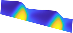
A sketch of the model geometry. The complex fluid has depth  $h(x,t)$ and a frictional contact density described by a spatially varying order parameter
 $\lambda (x,z,t)$ (represented by the colour map).

Assuming that the fluid is incompressible and inertia is negligible, conservation of mass and momentum demand that
 \begin{equation} \frac{\partial{{\hat{u}}}}{\partial{{\hat{x}}}} + \frac{\partial{{\hat{w}}}}{\partial{{\hat{z}}}} = 0 \end{equation}
and
 \begin{equation} \boldsymbol{0} = \rho {\boldsymbol{g}} - \boldsymbol{\nabla} {\hat{p}} + \boldsymbol{\nabla} \boldsymbol{\cdot} \hat{\boldsymbol{\tau}}, \end{equation}
where  ${\hat {p}}$ is the pressure,
 $\rho$ is the density, and
 ${\boldsymbol {g}} = (g \sin {\theta }, 0, -g \cos {\theta })$, with constant gravitational acceleration
 $g$ (we use the hat notation to denote dimensional variables; this decoration is removed below using suitable scalings to arrive at our dimensionless model). We take the deviatoric stress
 $\boldsymbol {{\hat {\tau }}}=\{{\hat {\tau }}_{ij}\}$ to be related to the rate of strains by the generalized Newtonian fluid model
 \begin{equation} {\hat{\tau}}_{ij} = {\hat{\mu}}(\lambda) \hat{\dot{\gamma}}_{ij} , \end{equation}
where
 \begin{equation} \hat{\dot{\boldsymbol{\gamma}}} = \{\hat{\dot{\gamma}}_{ij}\} = \boldsymbol{\nabla} \hat{\boldsymbol{u}} + (\boldsymbol{\nabla} \hat{\boldsymbol{u}})^{\rm T} , \end{equation}
and the second invariants of the tensors are  $\hat {\dot {\gamma }} = \sqrt {\frac 12\hat {\dot {\gamma }}_{ij}\hat {\dot {\gamma }}_{ij}}$ and
 ${\hat {\tau }} = \sqrt {\frac 12{\hat {\tau }}_{ij}{\hat {\tau }}_{ij}}$. The viscosity
 ${\hat {\mu }}(\lambda )$, is controlled by the parameter
 $\lambda ({\hat {x}},{\hat {z}},{\hat {t}})$.
At  ${\hat {z}}=0$ we adopt the no-slip condition. At the top surface
 ${\hat {z}}={\hat {h}}({\hat {x}},{\hat {t}})$, we ignore surface tension (in view of the relatively large scale of the films and waves featuring in experiments; see § 2.5), and adopt stress-free conditions. Thus
 \begin{equation} \boldsymbol{{\hat{u}}} = 0 \quad \text{at}\ {\hat{z}} = 0, \quad ({\hat{\tau}}_{ij} - {\hat{p}} \delta_{ij})n_j = 0 \quad \text{at}\ {\hat{z}} = {\hat{h}}({\hat{x}},{\hat{t}}), \end{equation}
where  $\boldsymbol {n}$ is the normal to the surface
 ${\hat {z}} = {\hat {h}}$. The kinematic condition implies
 \begin{equation} \frac{\partial{{\hat{h}}}}{\partial{{\hat{t}}}} + {\hat{u}} \frac{\partial{{\hat{h}}}}{\partial{{\hat{x}}}} = {\hat{w}} \quad \text{at} \ {\hat{z}} = {\hat{h}}({\hat{x}},{\hat{t}}). \end{equation}
2.2. Dimensionless leading-order formulation
To remove the dimensions from the equations, we introduce the scalings
 $$\begin{gather} {\hat{t}} = \frac{{\mathcal{L}}}{{\mathcal{U}}}t,\quad {\hat{x}} = {\mathcal{L}} x, \quad ({\hat{z}},{\hat{h}}) = {\mathcal{H}}(z,h), \end{gather}$$
 $$\begin{gather}{\hat{u}} = {\mathcal{U}} u, \quad {\hat{w}}=\varepsilon {\mathcal{U}} w,\quad {\hat{p}} = \rho g {\mathcal{H}} p \cos{\theta}, \quad {\hat{\tau}}_{ij} = \frac{\mu _{o} {\mathcal{U}}}{{\mathcal{H}}}\tau_{ij}, \quad {\hat{\mu}} = \mu _{o} \mu, \end{gather}$$
where  $\mu _{o}$ is a characteristic viscosity, and
 \begin{equation} {\mathcal{U}} = \frac{{\mathcal{H}}^3 \rho g}{{\mathcal{L}} \mu _{o}} \cos{\theta}.\end{equation}
With these scalings, and to leading order in  $\varepsilon$, (2.3) reduces to the lubrication equations
 \begin{equation} 0 = 1 - \frac{\partial{p}}{\partial{x}} + \frac{\partial{\tau_{xz}}}{\partial{z}} ,\quad 0 ={-}1 -\frac{\partial{p}}{\partial{z}}. \end{equation}
The dominant component of the rate of strain tensor is  $\dot {\gamma }_{xz} = \partial u/\partial z+O(\varepsilon ^2)$. Therefore, to leading order, the stress conditions in (2.5b) become
 \begin{equation} p= \tau_{xz} = 0 \quad \text{at} \ z=h(x,t). \end{equation}
The kinematic condition (2.7) is unchanged after scaling, but for the removal of the hats.
Equations (2.11) and (2.12) imply that the pressure is hydrostatic
 \begin{equation} p = h - z, \end{equation}
and the shear stress is given by
 \begin{align} \tau_{xz} &= (h-z)\left(1-\frac{\partial h}{\partial x}\right) \nonumber\\ &= \mu(\lambda)\frac{\partial u}{\partial z}. \end{align}
We write the shear stress in terms of its basal value
 \begin{equation} \tau_{xz} = (1-\zeta) \tau_b, \quad \tau_b = h \left(1-\frac{\partial h}{\partial x}\right) , \ \zeta = \frac{z}{h} .\end{equation}
In the shallow limit, the tensor invariants become approximated by  $\tau \approx |\tau _{xz}|$ and
 $\dot \gamma \approx |\dot \gamma _{xz}| \approx |\partial u / \partial z|$.
Finally, mass conservation integrated over the fluid layer implies
 \begin{equation} \frac{\partial{h}}{\partial{t}} + \frac{\partial{}}{\partial{x}}\int_0^h u \,{\rm d} z = \frac{\partial{h}}{\partial{t}} + \frac{\partial{}}{\partial{x}}\int_0^h(h-z)\frac{\partial{u}}{\partial{z}}\,{\rm d} z= 0. \end{equation}
Given
 \begin{equation} \frac{\partial{u}}{\partial{z}} \approx \dot\gamma = \frac{\tau}{\mu}, \end{equation}
we may substitute the relevant constitutive law into the final integral in (2.16) to arrive an evolution equation for the fluid thickness. Unfortunately, this reduction is complicated by the order parameter  $\lambda$ which, in general, retains an unknown spatial profile and satisfies its own evolution equation, as discussed below.
2.3. Constitutive model
In Darbois Texier et al.'s formulation of the Wyart & Cates's model, the order parameter  $\lambda (x,z,t)$ is identified as the local density of frictional contacts. In steady uniform shear, this density is dictated by the local shear stress:
 $\lambda = {\rm e}^{-\tau _*/\tau }$, where
 $\tau _*$ represents the characteristic stress for which short-range repulsion can be breached. Following earlier work (Chacko et al. Reference Chacko, Mari, Cates and Fielding2018; Richards et al. Reference Richards, Royer, Liebchen, Guy and Poon2019; Darbois Texier et al. Reference Darbois Texier, Lhuissier, Metzger and Forterre2023), we allow for both relaxation and diffusion of the frictional contacts by replacing the steady uniform shear relation by the evolution equation
 \begin{equation} \frac{\partial{\lambda}}{\partial{{\hat{t}}}}+ {\hat{u}}\frac{\partial{\lambda}}{\partial{{\hat{x}}}}+ {\hat{w}}\frac{\partial{\lambda}}{\partial{{\hat{z}}}} = \beta \dot\gamma \left[\exp\left(-\frac{\tau_*}{{\hat{\tau}}}\right) - \lambda\right] + K \nabla^2 \lambda , \end{equation}
where the relaxation rate is dictated by a multiple  $\beta$ of the local shear rate, and the diffusivity is
 $K$. The fluid rheology is then set by the viscosity law
 \begin{equation} \left.\begin{array}{ll@{}}
{\hat{\tau}} = {\hat{\mu}} \hat{\dot{\gamma}}, \quad
{\hat{\mu}} = {\mu _{o}\lambda_{o}^2}{({\lambda_{_O}} -
\lambda )^{{-}2}}, & \lambda < {\lambda_{_O}}, \\
\hat{\dot{\gamma}} = 0, & \lambda = {\lambda_{_O}},
\end{array}\right\} \end{equation}
where the characteristic viscosity  $\mu _{o}$ is related to the solvent viscosity constant
 $\eta _s$ defined by Darbois Texier et al. by
 \begin{equation} \mu _{o}= \frac{\eta_s}{(\phi_0-\phi)^2} . \end{equation}
In the model proposed by Wyart & Cates (Reference Wyart and Cates2014), the jamming fraction  ${\lambda _{_O}}$ is determined with reference to solid fraction
 $\phi$ and two other parameters
 \begin{equation} {\lambda_{_O}} = \frac{\phi_0 - \phi}{\phi_0-\phi_1} , \end{equation}
where  $\phi _0$ and
 $\phi _1$ are the jamming fractions for suspensions of frictionless and frictional particles, respectively. However, for the constitutive relation (2.19), all we require is the parameter
 ${\lambda _{_O}}$, in addition to the characteristic viscosity
 $\mu _{o}$.
Scaling as in § 2, we arrive at the (leading-order) dimensionless constitutive model for a thin film
 \begin{equation} {\mathcal{T}} \left( \frac{\partial{\lambda}}{\partial{t}}+ u\frac{\partial{\lambda}}{\partial{x}}+ w\frac{\partial{\lambda}}{\partial{z}} \right) = {\dot{\gamma}} \left[\exp\left(-\frac{\varUpsilon}{\tau}\right) - \lambda\right] + \kappa \frac{\partial^2\lambda}{\partial z^2} , \end{equation}
and
 \begin{equation} {\dot{\gamma}} = \tau \max\left(0, 1 - \frac{\lambda}{{\lambda_{_O}}}\right)^2 , \end{equation}
where the switch in (2.23) takes care of the yield condition implied by (2.19). Here, in order to ensure that the model combines time-dependent relaxation and vertical diffusion with the breaching of short-range repulsion, we have assumed that the following dimensionless groups are all order one:
 \begin{equation} {\mathcal{T}} = \frac{\varepsilon}{\beta} = \frac{{\mathcal{H}}}{{\mathcal{L}}\beta}, \quad \varUpsilon = \frac{{\mathcal{H}}\tau_*}{\mu _{o}{\mathcal{U}}} = \frac{\tau_*}{\rho g {\mathcal{H}} \tan\theta} , \quad \kappa = \frac{K}{\beta{\mathcal{U}}{\mathcal{H}}} . \end{equation}
In other words, the model corresponds to a particular distinguished limit of the physical parameters of the problem, and shares common points with other models used for thixotropic fluids (e.g. Mewis & Wagner Reference Mewis and Wagner2009; Hewitt & Balmforth Reference Hewitt and Balmforth2013; Larson & Wei Reference Larson and Wei2019). The thin-film theory that combines the constitutive law in (2.22)–(2.23) with (2.16) is similar to shallow ice models that explore thermo-viscous instabilities in glaciers (e.g. Clarke et al. Reference Clarke, Nitsan and Paterson1977; Hindmarsh Reference Hindmarsh2004).
The introduction of the diffusion term demands the addition of further boundary conditions for  $\lambda (x,z,t)$. We adopt the no-flux conditions
 \begin{equation} \frac{\partial{\lambda}}{\partial{z}} = 0 \quad {\rm at} \ z=0 \ \& \ z=h, \end{equation}
corresponding to the physical statement that frictional contacts between particles are neither created nor eliminated at the fluid surfaces. One might imagine that interfacial interactions could adjust contact densities locally, but without any further physical input, the no-flux condition seems least divisive.
2.4. The flow curve
The flow curve of a model fluid corresponds to the manner in which the shear stress  $\tau$ depends on shear rate
 ${\dot {\gamma }}$, under conditions of steady uniform shear. For the current constitutive law, the inverse of the flow curve can be expressed as
 \begin{equation} \dot\gamma = \tau \left[ 1 - {\lambda_{_O}}^{{-}1} \exp\left(-\frac{\varUpsilon}{\tau}\right) \right]^2 , \end{equation}
which is illustrated for a range of values of  ${\lambda _{_O}}$ (and
 $\varUpsilon =\frac 12$) in figure 2. At lower volume fractions, or higher values of
 ${\lambda _{_O}}$ (redder curves), the flow curve is monotonic; the viscosity increases smoothly with
 ${\dot {\gamma }}$, displaying a modest amount of continuous shear thickening. By contrast, at higher volume fraction, or lower
 ${\lambda _{_O}}$ (bluer curves), the flow curve bends back on itself at higher stresses to create distinctive non-monotonic stress–strain-rate curves. The criterion for the flow curve to fold back on itself is
 ${\lambda _{_O}}<2\textrm {e}^{-1/2}\approx 1.2131$. When this condition is met, the branches of the flow curve with negative slope are interpreted to be unstable, and any increase in shear rate past the turn back of the curve must prompt sudden, or discontinuous shear thickening. Such behaviour sets the scene for wave formation on inertialess films (Darbois Texier et al. Reference Darbois Texier, Lhuissier, Forterre and Metzger2020, Reference Darbois Texier, Lhuissier, Metzger and Forterre2023).
Flow curves in steady uniform shear for  $\varUpsilon =\frac 12$ and
 ${\lambda _{_O}}=0.4$,
 $0.75$,
 $0.95$, 1,
 $1.02$,
 $1.05$,
 $1.15$,
 $1.35$ and
 $2$ (increasing from blue to red, or as indicated by the arrow).

When  $1<{\lambda _{_O}}<2\textrm {e}^{-1/2}$, the folded back part of the flow curve eventually reaches a second fold point and then turns back to return to higher shear rate. The flow curve then adopts a characteristic S-shape with multiple stable branches over a range of shear rates. For
 ${\lambda _{_O}}<1$, however, the bent-back flow curve meets the yield point,
 ${\dot {\gamma }}=0$ and
 $\tau =\tau _{Y}=-\varUpsilon /\ln {\lambda _{_O}}$, without turning at a second fold point; for
 $\tau <\tau _{Y}$ the material does not deform.
Darbois Texier et al. (Reference Darbois Texier, Lhuissier, Metzger and Forterre2023) fit the flow curve in (2.26) to rheometer measurements of the suspensions that they use for flowing cornstarch experiments. Those fits work well when the shear thickening is continuous ( ${\lambda _{_O}}>2\textrm {e}^{-1/2}$), or up to the first turnaround of the flow curve when thickening is discontinuous (
 ${\lambda _{_O}}<2\textrm {e}^{-1/2}$). The bent-back portion of the flow curve is not calibrated in their rheometry, and no upper branch of an S-shaped curve was reliably found. Indeed, there is some controversy in the recent literature on discontinuous shear thickening as to whether a fluid-like upper branch even exists (Mari et al. Reference Mari, Seto, Morris and Denn2015b; Morris Reference Morris2020). Caution should therefore be exercised in adopting constitutive models like (2.22)–(2.23), particularly at higher stress levels. Here, we press on with the model in order to examine more closely its predictions for the dynamics of inertialess thin films, noting only that the stress levels attained never reach much beyond the first turnaround of the flow curve.
Note that the dimensionless model reduces to a Newtonian flow law by taking the limit,  ${\lambda _{_O}}\to \infty$. The flow curve also becomes Newtonian when
 $(\varUpsilon /\tau )\to \infty$ or
 $(\varUpsilon /\tau )\to 0$, although the two limits have a different effective viscosity. Nevertheless, unless both
 ${\mathcal {T}}$ and
 $\kappa$ also vanish, frictional contacts can still evolve in those two limits leading to time-dependent rheology.
2.5. Parameter settings
In addition to the dimensionless diffusivity  $\kappa$, the model in (2.15), (2.16), (2.22) and (2.23) contains three dimensionless rheological parameters,
 $\varUpsilon$,
 ${\mathcal {T}}$ and
 ${\lambda _{_O}}$. These parameters correspond to the stress needed for frictional contact, the relaxation time and the jamming threshold, respectively. In view of the definitions (2.21) and (2.24), suspensions prepared with varying solid fraction
 $\phi$ possess different values for
 ${\lambda _{_O}}$, but the same
 $\varUpsilon$ and
 ${\mathcal {T}}$.
Based on their rheometry, Darbois Texier et al. (Reference Darbois Texier, Lhuissier, Metzger and Forterre2023) quote  $\phi _0=0.52$,
 $\phi _1=0.43$,
 $\eta _s=9.1\times 10^{-4}$ Pa s and
 $\tau _*=12$ Pa, using a range of solid fractions
 $0.3\leq \phi \leq 0.47$. Their film experiments have mean depths of 1 cm or less. Such values imply that the parameter
 ${\lambda _{_O}}$ lies over the range 0.56–2.44, and
 $\varUpsilon \approx \frac 12$, which guide our parameter choices in figure 2 and hereon. For the relaxation time, Darbois Texier et al. did not measure any particular value, but quote estimates for frictional spheres from previous work (Chacko et al. Reference Chacko, Mari, Cates and Fielding2018; Richards et al. Reference Richards, Royer, Liebchen, Guy and Poon2019) of
 $\beta =10-10^{2}$, translating to dimensionless relaxation times of order
 $10^{-2}-10^{-3}$. As we shall see below in § 4, small values of
 ${\mathcal {T}}$ are problematic in the thin-film model (the distinguished limit taken in that model, in which
 ${\mathcal {T}}$ is taken to be order one, is also called into question, although one must simply set
 ${\mathcal {T}}=0$ when
 $\beta \gg \varepsilon$). In view of this, and the lack of any calibration, we leave open the choice for this parameter, along with that for
 $\kappa$. This dimensionless diffusivity is introduced chiefly so that vertical diffusion may assist in curing any mathematical problems in our thin-film theory, not necessarily as the gauge of a real physical effect. For that reason, we monitor the effect of varying this parameter, but mostly treat it as small.
3. Equilibria and linear stability
3.1. Base states
Solutions with the form of a steady sheet flow are given by
 \begin{equation} u=U(z), \quad \lambda = \varLambda(z), \quad \tau=1-z, \end{equation}
where the profiles  $U(z)$ and
 $\varLambda (z)$ follow from
 \begin{equation} U_z = (1-z) \max\left(0,1-\frac{\varLambda}{{\lambda_{_O}}}\right)^2, \quad \varLambda_{zz} = \frac{U_z}{\kappa} [{\rm e}^{-\varUpsilon/(1-z)} - \varLambda], \end{equation}
with  $U(0)=\varLambda _z(0)=\varLambda _z(1)=0$. Sample solutions to the prescribed-stress problem in (3.1) are displayed in figure 3. Examples with four values
 ${\lambda _{_O}}$ are presented, taking
 $\varUpsilon =\frac 12$, and diffusion constants of
 $\kappa =3\times 10^{-4}$ or
 $\kappa =0$. Because the stress
 $\tau =1-z$ increases monotonically on descending through the fluid layer, shear thickening occurs primarily near the underlying plane, and becomes most pronounced for the lowest values of
 ${\lambda _{_O}}$ (highest solid fractions).
(a) Flow profile,  $U(z)$, and (b) order parameter,
 $\varLambda (z)$, for steady uniform films with
 $\varUpsilon =\frac 12$,
 $\kappa =3\times 10^{-4}$ and
 ${\lambda _{_O}}=0.4$,
 $0.75$, 1 and
 $1.35$ (all solid blue). The (red) dashed lines show the solutions with
 $\kappa =0$. The inset replots the solutions on the
 $({\dot {\gamma }},\tau )$-plane and compares them with the steady-shear flow curves. The square for
 ${\lambda _{_O}}=0.4$ and
 $\kappa =0$ indicates the yield surface where
 $\varLambda ={\lambda _{_O}}$.

For  ${\lambda _{_O}}\gg 1$, the flow profile limits to the Nusselt profile,
 $U=z-\frac 12 z^2$, of a Newtonian fluid. With
 $\kappa =0$, on the other hand, we find the explicit solution
 \begin{align} U(z) = \int_0^z
(1-\tilde{z}) \left[ {\rm max} \left(0, 1 - \lambda_{_O}^{-1} {\rm e}^{-\varUpsilon/(1-z)} \right) \right]^2 \,{\rm d}\tilde{z} ,\quad
\varLambda(z) = \min({\lambda_{_O}}, {\rm
e}^{-\varUpsilon/(1-z)}).
\end{align}
The numerically computed solutions for  $\kappa =3\times 10^{-4}$ closely track this diffusionless solution in figure 3, except near the top and lower surfaces, where the no-flux condition exerts an effect, and for the case with
 ${\lambda _{_O}}=0.4$. For that lowest value of
 ${\lambda _{_O}}$, the diffusionless order parameter reaches the limit
 ${\lambda _{_O}}$ at a point within the fluid layer. This results in a yield surface below which material jams up and becomes rigid. With diffusion, however,
 $\varLambda (z)$ becomes smoothed and never reaches the yield point. When translated to loci on the
 $({\dot {\gamma }},\tau )$-plane (as in the inset to figure 3), the diffusionless solutions trace out part of the flow curve; the paths taken by the solutions with
 $\kappa =3\times 10^{-4}$ follow a similar vein.
For higher diffusivities  $\kappa$, the order parameter becomes more significantly smoothed, reducing the spatial viscosity variation and lifting the portraits of the solutions on the
 $({\dot {\gamma }},\tau )$-plane away from the flow curves; see figure 4. Near
 $\kappa =0.02$, the smoothing removes any fold back of the stress–strain-rate curves, and for
 $\kappa >1$, diffusion becomes sufficient to render
 $\varLambda$ almost uniform across the film (given the no-flux boundary conditions). A Newtonian-like, strong-diffusion solution then emerges with
 \begin{equation} U\sim \left(z-\frac{1}{2} z^2\right) \max\left(0,1-\frac{\varLambda}{{\lambda_{_O}}}\right)^2, \quad \varLambda\sim 2\int_0^1 (1-z)\,{\rm e}^{-\varUpsilon/(1-z)}\,{\rm d} z . \end{equation}
Note that (3.1) predicts that the limiting order parameter  $\varLambda$ exceeds
 ${\lambda _{_O}}$ for
 ${\lambda _{_O}}<0.44321$, implying that the entire layer plugs up with sufficient diffusion.
(a) Flow profile,  $U(z)$, (b)
 $\varLambda (z)$, and (c) portraits on the
 $({\dot {\gamma }},\tau )$-plane for steady uniform film solutions with
 $\varUpsilon =\frac 12$ and three values of
 ${\lambda _{_O}}$ and
 $\kappa$ (as indicated, and colour coded by
 $\kappa$). The dashed (green) lines show the limits for
 $\kappa \gg 1$.

3.2. Linear stability analysis
Infinitesimal perturbations to the base states above, with
 \begin{equation} h = 1+{\check\eta} \,{\rm e}^{{\rm i}kx+\sigma t}, \quad u = U(z)+\psi_z(z) \,{\rm e}^{{\rm i}kx+\sigma t}, \quad \lambda = \varLambda(z)+{\check\lambda}(z) \,{\rm e}^{{\rm i}kx+\sigma t}, \end{equation}
wavenumber  $k$ and (complex) growth rate
 $\sigma =\sigma _r+i\sigma _i$, satisfy
 $$\begin{gather} [\sigma + {\rm i}k U(1)] {\check\eta} ={-}{\rm i}k \psi(1), \end{gather}$$
 $$\begin{gather}\psi_{zz} = \left( 1 - \frac{\varLambda}{{\lambda_{_O}}}\right)^2 {\check\tau} - \frac{2}{{\lambda_{_O}}}(1-z) \left( 1 - \frac{\varLambda}{{\lambda_{_O}}}\right) {\check\lambda} , \end{gather}$$
 $$\begin{gather}{\mathcal{T}} [ (\sigma+{\rm i}kU) {\check\lambda} - {\rm i}k \varLambda_z\psi ] = \frac{\varUpsilon U_z {\check\tau} \,{\rm e}^{-\varUpsilon/(1-z)}}{(1-z)^2} + [{\rm e}^{-\varUpsilon/(1-z)} - \varLambda] \psi_{zz} - U_z {\check\lambda} + \kappa {\check\lambda}_{zz} . \end{gather}$$
Here,  $\psi (z)$ represents a streamfunction such that
 $(u,w)=(U+\psi _z\,\textrm {e}^{\textrm {i}kx+\sigma t},-\textrm {i}k\psi \,\textrm {e}^{\textrm {i}kx+\sigma t})$, and the shear stress perturbation has amplitude
 \begin{equation} {\check\tau} = [1 - {\rm i}k(1-z)]{\check\eta}. \end{equation}
The boundary conditions translate to  $\psi (0)=\psi _z(0)={\check \lambda }_z(0)={\check \lambda }_z(1)=0$.
Numerical results of the linear stability analysis are shown in figure 5, which plots the growth rate of the most unstable mode against wavenumber  $k$ for
 $(\kappa,{\mathcal {T}},\varUpsilon )=(10^{-3},10^{-2},\frac 12)$ at several values of
 ${\lambda _{_O}}$. With the highest values of
 ${\lambda _{_O}}$ of
 $1.2<2\textrm {e}^{-1/2}$ and
 $1.35$ (the lowest solid fractions; redder curves), all modes are stable, even though the base state for the first of these values possesses an S-shaped flow curve. The lower values of
 ${\lambda _{_O}}$ (higher solid fractions; bluer curves) are unstable for wavenumbers below a critical cutoff
 $k=k_{crit}$. The growth rate is maximized at the particular wavenumber
 $k=k_{max}$ indicated in the plots. As illustrated in figure 5(a,b) and discussed below in § 4.1, the growth rate and phase speed for
 $k\to 0$ can be predicted analytically.
(a) Growth rate,  $\sigma _r$, and (b) scaled phase speed,
 $-\sigma _i/(kU_*)$, against wavenumber
 $k$ for
 $(\kappa,{\mathcal {T}},\varUpsilon )=(10^{-3},10^{-2},\frac 12)$ and
 ${\lambda _{_O}}=\{\frac 34,\frac 78,1,1.1,1.2,1.35\}$ (from blue to red). Scaled phase speeds are shown only where
 $\sigma _r>-2$. The dashed line in (b) shows the prediction in (4.5) of § 4.1. The corresponding prediction for the growth rate is included in the inset of (a), which plots
 $\sigma _r/k^2$ for smaller wavenumber. The stars show the most unstable modes for
 ${\lambda _{_O}}<1.2$; the corresponding eigenfunctions,
 $\psi _z(z)$ and
 ${\check \lambda }(z)$, are shown in (c) and (d), normalized so that
 ${\check \eta }=1$; the real parts are shown by solid lines and the imaginary parts as dashed lines.

The most unstable modes have eigenfunctions (shown in figure 5c,d) which are characterized by strong perturbations in  $\lambda$ over the lower part of the fluid layer. These variations are predominantly opposite to the perturbations in speed
 $\psi _z$ and surface slope
 $\textrm {i}k{\check \eta }$. Such features imply that a local upturn in surface slope, corresponding to a local decrease in stress, weakens
 $\lambda$ and thence viscosity, to accelerate flow. Conversely, a local downturn in surface slope leads to an increasing stress, the strengthening of
 $\lambda$ and flow deceleration. In combination, wavey perturbations become amplified. In other words, the perturbations harness a material response mirroring the fold back of the flow curve for
 ${\lambda _{_O}}<2\textrm {e}^{-1/2}$, as described previously by Darbois Texier et al. (Reference Darbois Texier, Lhuissier, Forterre and Metzger2020).
Growth rates and phase speeds for varying  ${\lambda _{_O}}$ and
 ${\mathcal {T}}$ are plotted in figure 6. The degree of instability increases continually as the relaxation time decreases, indicating a singular limit for
 ${\mathcal {T}}\to 0$. Conversely, the instability becomes suppressed for sufficiently large relaxation time. The onset of instability also occurs for finite wavenumber as
 ${\lambda _{_O}}$ decreases below
 $\textrm {e}^{-1/2}$, most noticeably for higher
 ${\mathcal {T}}$. The phase speeds,
 $-\sigma _i/k$, plotted in figures 5 and 6 are scaled by the mean speed (flux) of the base solutions
 \begin{equation} U_* = \int_0^1 U(z)\, {\rm d} z. \end{equation}
At very low wavenumbers, and for smaller relaxation times, instability first appears for modes with phase speeds that are roughly twice the mean flow speed. This feature is discussed further below in § 4, and was exploited by Darbois Texier et al. to rationalize experimental observations. However, the most unstable modes over all wavenumbers have rather lower phase speeds, closer to and often less than the mean flow speed.
(a) Growth rate,  $\sigma _r$, and (b) scaled phase speed,
 $-\sigma _i/(kU_*)$, plotted as densities on the
 $(k,{\lambda _{_O}})$-plane, with
 $(\kappa,\varUpsilon )=(10^{-3},\frac 12)$, and
 ${\mathcal {T}}=10^{-3}$,
 $10^{-2}$,
 $0.1$ and
 $\frac 12$ (from right to left). The thicker red lines indicate the most unstable wavenumber
 $k_{max}$ for each
 ${\lambda _{_O}}$. The colour scales saturate at negative growth rates.

Growth rates as a function of  $k$ and
 $\kappa$ at fixed
 ${\lambda _{_O}}=1$ and
 ${\mathcal {T}}=0.1$ are shown in figure 7. This plot extends from close to the diffusionless limit (
 $\kappa \to 0$), to the strongly diffusive limit (
 $\kappa \gg 1$). The stability problem simplifies somewhat in the first of these limits because
 ${\check \lambda }$ becomes determines algebraically from
 $\psi$ and
 ${\check \tau }$ in (3.8) (bearing in mind that
 $\varLambda \to \textrm {e}^{-\varUpsilon /(1-z)}$ for
 $\kappa \to 0$), and one must solve only (3.7). Further discussion of the opposite limit of strong diffusion is given below in § 5. Unexpectedly, perhaps, instability persists in this latter limit, extending to increasingly high wavenumbers as
 $\kappa$ is raised. In other words, the diffusion of frictional contacts does not suppress instability, even though a sufficient increase in
 $\kappa$ eliminates any turn back in the local
 $({\dot {\gamma }},\tau )$-relation of the base state (see figure 4).
Density plots of (a) growth rate,  $\sigma _r$, and (b) scaled phase speed,
 $-\sigma _i/(kU_*)$ above the
 $(k,\kappa )$-plane for unstable modes with
 $({\lambda _{_O}},{\mathcal {T}},\varUpsilon )=(1,0.1,\frac 12)$. The thicker red line indicates the most unstable wavenumber
 $k_{max}$ for each
 $\kappa$. The colour scales saturate at negative growth rates. Below are plots of (c,e)
 $\sigma _r$, and (d,f)
 $-\sigma _i/(kU_*)$ against
 $k$ for the values of
 $\kappa$ indicated. The dashed lines show the limits
 $\kappa \to \infty$ (see § 5) and
 $\kappa \to 0$.

4. Rapid relaxation,  ${\mathcal {T}}\ll 1$

With a relatively rapid relaxation of the frictional contacts ( ${\mathcal {T}}\to 0$), the order parameter becomes determined by solving
 \begin{equation} {\check\kappa} \lambda_{\zeta\zeta} = (1-\zeta) \left(1 - \frac{\lambda}{{\lambda_{_O}}}\right)^2 [\lambda - {\rm e}^{-{\check\Upsilon}/(1-\zeta)}], \end{equation}
with
 \begin{equation} \tau_b = h(1-h_x),\quad \zeta=\frac{z}{h},\quad {\check\Upsilon} = \frac{\varUpsilon}{\tau_b}, \quad {\check\kappa} = \frac{\kappa}{h^2\tau_b}, \quad \lambda_\zeta(0)=\lambda_\zeta(1)=0, \end{equation}
on assuming the yield condition is never met. This problem, however, is identical to that for the base states in § 3.1, but for the replacements  $\kappa \to {\check \kappa }$ and
 $\varUpsilon \to {\check \Upsilon }$. Hence, we may write the solutions to both problems in terms of a single function, as either
 $\lambda = \varLambda (\zeta ; \varUpsilon,\kappa )$ or
 $\lambda = \varLambda (\zeta ; {\check \Upsilon },{\check \kappa })$.
Of particular importance is the flux function
 \begin{align} \int_0^h u(x,z,t)\, {\rm d} z &=\int_0^1 (h-z) u_z \, {\rm d} z \nonumber\\ &= h^2\tau_b \int_0^1 (1-\zeta)^2 \left(1 - \frac{\lambda}{{\lambda_{_O}}}\right)^2 {\rm d}\zeta = h^2 \tau_b {\mathcal{Q}}({\check\Upsilon},{\check\kappa}) . \end{align}
Armed with this flux function, we may now turn to the conservation of mass relation (2.16) and write the single evolution equation
 \begin{equation} h_t + \left[h^3(1-h_x) {\mathcal{Q}}\left(\frac{\varUpsilon}{h(1-h_x)},\frac{\kappa}{h^3(1-h_x)}\right) \right]_x = 0. \end{equation}
Note that the base states of § 3.1 have a flux, or mean velocity, of  $U_* = {\mathcal {Q}}(\varUpsilon,\kappa )$.
4.1. Revisiting linear stability
By introducing  $h=1+{\check \eta } \,\textrm {e}^{-\textrm {i}kx+\sigma t}$ into (4.4) and linearizing, we arrive at
 \begin{equation} \sigma ={-}{\rm i}k (3U_*-\varUpsilon {\mathcal{Q}}_1-3\kappa {\mathcal{Q}}_2) + k^2 (\varUpsilon {\mathcal{Q}}_1 +\kappa {\mathcal{Q}}_2 - U_*), \end{equation}
where
 \begin{equation} {\mathcal{Q}}_1 = \left[ \frac{\partial{{\mathcal{Q}}}}{\partial{{\check\Upsilon}}} \right]_{h=1} \quad {\rm and} \quad {\mathcal{Q}}_2 = \left[ \frac{\partial{{\mathcal{Q}}}}{\partial{{\check\kappa}}} \right]_{h=1}, \end{equation}
are the partial derivatives of the flux function evaluated for the base state. As long as  $\varUpsilon {\mathcal {Q}}_1 +\kappa {\mathcal {Q}}_2 > U_*$, the base state is therefore unstable. The growth rate and phase speed predicted by (4.5) are included in figure 5. These predictions match up with the numerical solutions for
 $k\ll 1$ in these figures because relaxation is relatively rapid in the small-wavenumber limit.
For higher wavenumber, the predictions from (4.5) fail to match the drop off in linear instability observed for the numerical solutions in figure 5. In fact, (4.5) predicts an unbounded increase in growth rate with wavenumber, the hallmarks of an ultraviolet catastrophe. In other words, in the limit of rapid relaxation, the linear thin-film problem becomes ill posed with the shortest wavenumbers growing fastest. As illustrated by the numerical solutions of the linear stability problem in figures 5 and 6, this drawback is cured by a finite relaxation time. However, the approach to the singular limit  ${\mathcal {T}}\to 0$ is evident in figure 6, where the range of unstable wavenumbers and maximum growth rate diverge as the relaxation time is decreased.
4.2. No diffusion
With  $\kappa =0$, the calculation of the flux function becomes simpler. In this case,
 $\varLambda =\textrm {e}^{-{\check \Upsilon }/(1-\zeta )}$ and
 \begin{equation} G(\tau_b) = \tau_b {\mathcal{Q}}({\check\Upsilon},{\check\kappa}) = \tau_b \int_0^1 (1-\zeta)^2 \left(1 - \frac{\lambda}{{\lambda_{_O}}}\right)^2 {\rm d}\zeta \equiv \frac{1}{\tau_b^2} \int_0^{\tau_b} {\tilde\tau} \varGamma({\tilde\tau})\,{\rm d}{\tilde\tau} , \end{equation}
where  $\varGamma (\tau )=\tau (1-{\lambda _{_O}}^{-1}\,\textrm {e}^{-\varUpsilon /\tau })^2$ is the inverse of the flow curve function (cf. (2.26)), which can be written in terms of exponential integrals.
The lubrication model now becomes
 \begin{equation} h_t + [h^2 G(\tau_b)]_x = 0 , \end{equation}
so that the linear growth rate can be read off as
 \begin{equation} \sigma ={-}{\rm i}k [2G(1)+G'(1)] - k^2 G'(1) . \end{equation}
Linear instability arises for
 \begin{equation} G'(1) = \int_0^1 {\tilde\tau}^2 \varGamma'({\tilde\tau}) \,{\rm d}{\tilde\tau}<0 , \end{equation}
which is equivalent to the instability condition quoted by Darbois Texier et al. The condition does not quite match the criterion,  $\varGamma '(1)<0$, which indicates when the fluid at the bottom of the layer in the base flow lies beyond the first turnaround of the flow curve (although it is an integral average of
 $\varGamma '(\tau )$ that is weighted to the base of the fluid layer). Flux functions
 $G(\tau _b)$ for the same values of
 ${\lambda _{_O}}$ and
 $\varUpsilon$ as displayed in figure 2 are illustrated in figure 8; an inset compares the stability indicator
 $G'(1)$ with
 $\varGamma '(1)$. Note that
 $G'(1)$ is numerically small, which is the origin of Darbois Texier et al.'s conclusion that the phase speeds of unstable waves are close to twice the mean flow speed (here
 $2G(1)\equiv 2U_*$).


To summarize, without a finite relaxation time, the linearized inertialess thin-film model is ill posed (a feature that likely carries over to the nonlinear versions in (4.4) and (4.8)). One might imagine that relaxing the thin-film approximation or including inertia could cure this ultraviolet catastrophe. In fact, as we show in Appendix A, where we briefly advance beyond the inertialess, thin-film limit (but omit diffusion), neither of these extensions suffices; a finite relaxation time is still needed. Surface tension, which has been omitted here, offers another possible physical regularization. The inclusion of that effect modifies the base shear stress in thin-film theory so that  $\tau _b = h(1-h_x+{\mathcal {S}} h_{xxx})$, where
 ${\mathcal {S}}$ is a suitable, dimensionless, Bond number (the hydrostatic pressure being replaced by
 $p = h-z - {\mathcal {S}} h_{xx}$; e.g. Chang Reference Chang1994; Ruyer-Quil & Manneville Reference Ruyer-Quil and Manneville2000). With this inclusion, a repetition of the analysis above simply replaces the factor
 $k^2$ in (4.5) or (4.9) with
 $k^2+{\mathcal {S}} k^4$. The divergence of the growth rate with
 $k$ is therefore exacerbated by surface tension.
5. Strong diffusion, $\kappa \gg 1$

As remarked in § 3.1, when diffusion of frictional contacts is relatively strong  $\kappa \gg 1$ (and the boundary conditions on
 $\lambda$ are no flux),
 $\varLambda (z)$ becomes almost uniform across the film for the base states of the linear stability analysis. In fact, this feature carries over to the full thin-film problem, which simplifies further in this limit: integrating (2.22) across the film, and then introducing the approximation
 $\lambda \sim \lambda (x,t)$, we find
 \begin{equation} ( h \lambda )_t + \left( \lambda \int_0^h u\,{\rm d} z \right)_x = \frac{1}{{\mathcal{T}}} \left(1 - \frac{\lambda}{{\lambda_{_O}}}\right)_+^2 \int_0^h \tau ({\rm e}^{-\varUpsilon/\tau} - \lambda)\, {\rm d} z, \end{equation}
and
 \begin{equation} V = \frac{1}{h}\int_0^h u\,{\rm d} z = \frac{1}{3} h\tau_b \left(1 - \frac{\lambda}{{\lambda_{_O}}}\right)_+^2,\end{equation}
where we have employed the short-hand notation,  $\max (0,X)=(X)_+$. Hence
 \begin{equation} \left.\begin{array}{c}
h_t + (hV)_x= 0, \quad \tau_b = h(1-h_x),\\ \displaystyle
(h\lambda)_t + (hV\lambda)_x = \dfrac{3V}{2{\mathcal{T}}} [
E(\tau_b) - \lambda ] , \quad E(\tau_b) =
\dfrac{2}{\tau_b^2} \int_0^{\tau_{b}} {\tilde\tau} \,{\rm
e}^{-\varUpsilon/{\tilde\tau}} \,{\rm d} {\tilde\tau} .
\end{array}\right\} \end{equation}
For a steady, uniform base state,  $h(x,t)=1$ and
 $\lambda (x,t)=\varLambda$, we recover the order parameter in (3.1). The linear stability of these base states follows from setting
 $h=1+{\check \eta } \,\textrm {e}^{\textrm {i}kx+\sigma t}$ and
 $\lambda = \varLambda + {\check \lambda } \,\textrm {e}^{\textrm {i}kx+\sigma t}$, linearizing in the amplitudes
 ${\check \eta }$ and
 ${\check \lambda }$ and then solving a quadratic equation for the growth rate
 $\sigma$ stemming from (5.3). Sample results are plotted in figure 9 for
 $({\mathcal {T}},\varUpsilon )=(0.1,\frac 12)$. As
 ${\lambda _{_O}}$ is decreases through the critical value
 $\lambda _{_{SD}}(\varUpsilon )=4\textrm {e}^{-\varUpsilon }-3\varLambda <2\textrm {e}^{-1/2}$ (with
 $\lambda _{_{SD}}(\frac 12)\approx 1.0965$), instability sets in at the largest wavenumbers. An ultraviolet catastrophe is avoided, however, and
 \begin{equation} \sigma_r \to \frac{(\lambda_{_{SD}}-{\lambda_{_O}})({\lambda_{_O}}-\varLambda)} {2{\mathcal{T}}{\lambda_{_O}}^2} \quad {\rm and} \quad -\frac{\sigma_i}{kU_*} \to 1 \quad {\rm for} \ k\gg1 . \end{equation}
For  ${\lambda _{_O}}$ further below
 $\lambda _{_{SD}}$, all wavenumbers become unstable, but the shortest waves remain the fastest growing. The predictions for the strong-diffusion limit were also included earlier in figure 7(c,d) and compared with numerical results for the full thin-film model. Evidently, there is no selection of a preferred wavelength in linear theory and a pronounced dependence of the nonlinear dynamics on initial condition is suggested. Therefore, in the full thin-film model, a preferred wavelength arises due to the relaxation, but not diffusion, of
 $\lambda$.
(a) Growth rates  $\sigma _r$ and (b) scaled phase speeds,
 $\sigma _i/(kU_*)$ on the
 $(k,{\lambda _{_O}})$-plane in the strong-diffusion limit, for
 $\varUpsilon =\frac 12$ and
 ${\mathcal {T}}=0.1$.

The simplicity of the strong-diffusion equations (5.3) suggests an avenue to interrogate the development of instabilities from low-amplitude, approximately linear perturbations into nonlinear waves. However, a device to limit the range of unstable wavenumbers is still required and the strong-diffusion limit, in which the frictional contact density becomes uniform across the depth of the fluid film, is itself probably unphysical. The exercise can nevertheless prove useful, permitting a certain amount of analytical headway into deciphering the nonlinear dynamics. In Appendix B, we follow this pathway, adding artificial diffusion-in- $x$ terms to remove instability at the highest wavenumbers. A notable feature exposed by this analysis is that the linear instability saturates at finite amplitude to form shock-like nonlinear waves, travelling at a speed that can be predicted analytically. The analysis further exposes how linear instability can extend into the limit of strong diffusion, even though the local stress–strain-rate relation of the base-flow profile is monotonic (cf. § 3.2).
6. Nonlinear waves
To provide an exploration of the nonlinear dynamics of unstable waves that avoids the strong-diffusion limit, we return to the full order parameter equation in (2.22) and capture the complete spatial dependence of  $\lambda (x,z,t)$. In Appendix C, we summarize the strategy we use to solve this problem numerically for spatially periodic domains of length
 $2{\rm \pi} /k$, with
 $k$ selected close to the wavenumber that is preferred when the relaxation time
 ${\mathcal {T}}$ and diffusivity
 $\kappa$ are finite.
Figure 10 displays a sample numerical solution. The initially small perturbation to the base state again amplifies exponentially according to the predictions of linear stability analysis (§ 3.2). Growth then saturates in the nonlinear regime, leading to the formation of a steadily propagating wave. The nonlinear wave travels slightly more slowly than the linear wave speed, which is in turn slightly slower than the mean flow. This dynamics matches that found in the strong-diffusion limit (see Appendix B), although the nonlinear wave profile in figure 10 is relatively smooth and shows no tendency to form a shock. The fall of the profile beyond the crest does, however, become somewhat steeper than the preceding rise. Note that computations are continued only up to times just beyond where linear instability saturates; any subsequent nonlinear dynamics, such as secondary instabilities, is not captured.
Nonlinear solution for  $({\lambda _{_O}},{\mathcal {T}},\kappa,k,A)=(1,0.1,10^{-3},10,2\times 10^{-4})$. (a) Snapshots of
 $\lambda (x,z,t)$ at five successive times (as indicated by the stars in (c)). The solutions are mapped onto the inclined plane. (b) The free surface position
 $h(x,t)$, shown in the frame of the final nonlinear wave, with spatial coordinate
 $\xi =k(x-c_nt)$, where
 $c_n\approx 0.05\approx 0.55U_*$. (c) Time series of the mean surface displacement
 $\sqrt {\langle (h-1)^2\rangle }$ (where
 $\langle \cdots \rangle$ denotes an average in
 $x$). The dashed line shows the growth predicted by linear stability analysis.

At early times, when the film is similar to the uniform base flow, the order parameter  $\lambda (x,z,t)$ is enhanced over the lower parts of the film by the elevated shear stress there. As the nonlinear wave develops, the flattening of the surface over the rise of the wave reduces the shear stress to lower
 $\lambda$ locally. Shear thickening then takes place primarily underneath the fall of the wave profile, enhancing the viscosity there to create the distinctive pattern in
 $\lambda$ seen in the snapshots in figure 10(a).
Further details of the final, steady nonlinear wave are shown in figure 11. In the first panel, a density map of  $\lambda$ is compared with contours of constant
 $\textrm {e}^{-\varUpsilon /|\tau |}$. Although the two are not perfectly aligned, the trends of both are similar, indicating that the local relation between
 $\dot \gamma$ and
 $\tau$ lies near, but does not follow, the steady-state flow curve. Shear thickening takes place primarily within the region where the stress exceeds the threshold,
 $|\tau |\approx 0.4$, implied by the first turn back of the flow curve (the black contour in figure 11a). The streamline plot in the second panel of figure 11 illustrates how the shear thickening and step conspire to create a recirculating cell underneath the crest of the nonlinear wave.
The final nonlinear wave from figure 10, showing (a) contours of constant  $\textrm {e}^{-\varUpsilon /|\tau |}$, superposed on a density map of
 $\lambda$, and (b) a selection of streamlines, superposed on a density map of
 $u/U_*$. Both are shown in the frame of the wave, with streamwise coordinate
 $\xi =k(x-c_nt)$. The black curve in (a) shows the contour
 $|\tau |\approx 0.4$, the stress above which discontinuous shear thickening is expected (cf. figures 2 and 3).

A selection of steady nonlinear wave profiles for varying  ${\lambda _{_O}}$ is shown in figure 12(a). As this parameter decreases and the linear instability becomes stronger, the wave height (measured in figure 12 as
 $\max (h)-\min (h)$) increases. Tracing the wave profiles back up to the onset of linear instability at larger
 ${\lambda _{_O}}$ suggests a supercritical transition (see panel b). At the smaller values of
 ${\lambda _{_O}}$, the nonlinear wave profile develops into relatively steep steps separated by long, almost linear sections. Below the steps, fluid discontinuously shear thickens throughout almost its entire depth, whereas the wave profile become almost flat between the steps, reflecting a very low shear stress. In other words, fluid gravitationally pools behind the sharp, shear-thickened steps, which implies that those features present effective barriers to the film flow.
(a) Steady nonlinear wave profiles for  $({\mathcal {T}},k,\varUpsilon,\kappa )=(0.1,10,\frac 12,10^{-3})$ and
 ${\lambda _{_O}}=\{0.9,1,1.05,1.07\}$ (colour coded, from red to blue). The profiles are plotted so that their crests are aligned, and the triangle shows unit slope (
 $h_x=1$). (b) Wave height,
 $\max (h)-\min (h)$, against
 ${\lambda _{_O}}$, for a wider set of computations. The stars indicate the values for
 ${\lambda _{_O}}$ in (a,b), and the vertical dot-dashed line indicates the linear stability boundary. The inset density plots show
 $\lambda (x,t)$ for the values of
 ${\lambda _{_O}}$ indicated.

The reduction of the net flux by the nonlinear waves is illustrated further in figure 13, which displays time series of the horizontal averages of the surface and depth-averaged speed  $u$ for the solutions also shown in figure 12. In all four examples, the net flow speed is reduced by the nonlinear wave, although the effect is minor near the linear stability threshold (for
 ${\lambda _{_O}}=1.07$). The instantaneous wave speed (measured using the position at the core of the wave where
 $h=1$ and
 $h_x<0$) is smaller still. At early times, this wave speed matches the prediction of linear theory, then falls sharply as the wave saturates, before converging to the final nonlinear wave speed
 $c_n< U_*$.
(a) Time series of three scaled speeds for  $({\mathcal {T}},k,\varUpsilon,\kappa )=(0.1,10,\frac 12,10^{-3})$ and
 ${\lambda _{_O}}=\{0.9,1,1.05,1.07\}$ (colour coded, from red to blue). The solid line shows the depth and
 $x$-averaged speed,
 $\langle h^{-1} \int _0^h u(x,z,t) \,\textrm {d} z \rangle$, the dashed line show the
 $x$-averaged surface speed,
 $\langle u(x,h,t) \rangle$, and the dotted line show the instantaneous wave speed (measured using the position where
 $h=1$ and
 $h_x<0$). All three are scaled by
 $U_*$. The stars indicate the final nonlinear wave speeds, which are plotted in (b) for a wider suite of computations. The vertical dot-dashed line again shows the linear stability threshold.

7. Discussion
The non-monotonic flow curves of certain complex fluids in steady, uniform shear can trigger hydrodynamic instabilities. For suspensions that display discontinuous shear thickening such as cornstarch, this effect plausibly rationalizes the large-amplitude waves seen on relatively slow, falling films (Darbois Texier et al. Reference Darbois Texier, Lhuissier, Forterre and Metzger2020, Reference Darbois Texier, Lhuissier, Metzger and Forterre2023). Here, we have examined a detailed theoretical model of such films, building on Darbois Texier et al.'s formulation of the constitutive law for steady, uniform shear proposed by Wyart & Cates (Reference Wyart and Cates2014). Employing that law for the local viscosity in an inertialess thin-film model is problematic: waves of all wavelength are predicted to be unstable, with a growth rate that diverges at high wavenumbers. We have demonstrated that the inclusion of both relaxation or diffusion across the film can control this ultraviolet catastrophe. On the other hand, neither inertia nor the extensional viscous stresses ignored in thin-film theory can cure the problem (a conclusion following from the extension of the thin-film model explored in Appendix A).
For the constitutive law that we have employed, relaxation removes unstable waves of small wavelength, to furnish a preferred wavenumber; diffusion, however, does not. The onset of linear instability sometimes, but not always, lies close to a long-wave stability criterion that can be established analytically. That criterion does not precisely coincide with the condition that the profile of the base flow samples the non-monotonic part of the flow curve under steady uniform shear, even in the limit that relaxation becomes arbitrarily fast. In fact, with a sufficiently long relaxation time, linear instability is suppressed altogether, even when discontinuous shear thickening arises in the base flow.
By solving the thin-film model numerically, we have constructed the steadily propagating nonlinear waves that result from the saturation of linear instability when disturbances reach finite amplitude. Changing the parameters of the constitutive law so that the rheology progresses from continuous to discontinuous shear thickening, we observe the emergence of low-amplitude waves on passing the linear instability threshold, in the usual manner of a supercritical transition. As the fluid becomes more shear thickening, the waves become stronger, taking the form of relatively steep steps, under which fluid is substantially thickened by elevated stresses. Between the steps, viscosity remains low and the fluid pools into long, almost flat, sections. Such phenomenology bears some similarities with that of the waves seen in laboratory experiments (Balmforth et al. Reference Balmforth, Bush and Craster2005; Darbois Texier et al. Reference Darbois Texier, Lhuissier, Forterre and Metzger2020, Reference Darbois Texier, Lhuissier, Metzger and Forterre2023). However, Balmforth et al. (Reference Balmforth, Bush and Craster2005) report that waves become very steep in front of their crests, often overturning there. Darbois Texier et al. do not comment on this aspect of their experiments, although the downward profiles of their ‘Oobleck waves’ also look to quickly steepen. Excessive wave steepening and overturning cannot be captured by the thin-film asymptotics inherent in the model presented here.
Similarly, the linear stability theory predicts that preferred wavelengths are relatively short, implying further limitations on thin-film theory: in the model, the dimensional wavelength,  $2{\rm \pi} k^{-1} {\mathcal {L}} = 2{\rm \pi} k^{-1} {\mathcal {H}} \cot \theta$, should greatly the fluid depth
 ${\mathcal {H}}$; i.e. the dimensionless wavenumber
 $k$ should be much less than
 $2{\rm \pi} \cot \theta$. For the slopes of the channels used in laboratory experiments (of order
 $10^\circ$), this translates to the constraint
 $k\ll O(30)$. Consequently, if relaxation times are relatively small, the predicted preferred wavelengths are too short to be accurately captured in the long-wave model (preferred wavenumbers are predicted to be
 $O(10)$ or smaller when
 ${\mathcal {T}}>0.1$).
The theoretically predicted linear wave speeds are also smaller than those observed experimentally by Balmforth et al. (Reference Balmforth, Bush and Craster2005) and Darbois Texier et al. (Reference Darbois Texier, Lhuissier, Forterre and Metzger2020, Reference Darbois Texier, Lhuissier, Metzger and Forterre2023), who both noted that waves travelled significantly faster than the mean flow. In the model, the waves travel closer to the mean flow speed (for finite relaxation time), unless the wavenumber is arbitrarily decreased below that of the most unstable mode. Moreover, because nonlinear waves invariably create shear-thickened barriers to flow, those disturbances invariably decelerate further on reaching finite amplitude in the model. It therefore seems challenging to explain the relatively fast experimental wave speeds. One immediate explanation for this discrepancy is that the spatially periodic setting and initialization of the model lead to differences with the experiments, in which waves develop along the channel from an inlet with its own dynamics.
In conclusion, thin-film theory incorporating instantaneous shear thickening within the framework of a generalized Newtonian fluid model predicts linearly unstable waves in the inertialess limit. However, this theory is not sufficient to explain the detailed properties (wavelengths and wave speeds) of the waves observed in flowing films of cornstarch solutions. Here, it has been shown that the addition of time-dependent relaxation of frictional contacts may partly help to save this situation. Overall, the instabilities observed on flowing films of discontinuously shear-thickening fluids provide interesting constraints on the underlying constitutive behaviour, as in some other flows cornstarch suspensions (e.g. Merkt et al. Reference Merkt, Deegan, Goldman, Rericha and Swinney2004; von Kann et al. Reference von Kann, Snoeijer, Lohse and van der Meer2011; Brown & Jaeger Reference Brown and Jaeger2014; Ovarlez et al. Reference Ovarlez, Le, Smit, Fall, Mari, Chatté and Colin2020; Bougouin et al. Reference Bougouin, Metzger, Forterre, Boustingorry and Lhuissier2024). In more general settings, one wonders whether phenomena of this kind act as practical rheometers to probe and inform the rheology of complex fluids or granular media (cf. Edwards & Gray Reference Edwards and Gray2015).
Acknowledgements
I thank the referees for their thoughtful comments which helped to improve the manuscript. I thank the Isaac Newton Institute for Mathematical Sciences, Cambridge, for support and hospitality during the programme ‘Anti-diffusive dynamics: from sub-cellular to astrophysical scales’ where part of the work on this paper was undertaken.
Funding
This work was supported by EPSRC grant no EP/K032208/1.
Declaration of interests
The author reports no conflict of interest.
Appendix A. Beyond the inertialess thin-film limit, with $\kappa =0$

Restoring inertia and the higher-order terms in  $\varepsilon$, the dimensionless conservation of momentum equations are
 $$\begin{gather} R (u_t + uu_x + wu_z) = \varepsilon \frac{\partial{\tau_{xx}}}{\partial{x}} + \frac{\partial{\tau_{xz}}}{\partial{z}} - \frac{\partial{p}}{\partial{x}} + 1, \end{gather}$$
 $$\begin{gather}\varepsilon^2 R (w_t + uw_x + ww_z) = \varepsilon^2 \frac{\partial{\tau_{xz}}}{\partial{x}} + \varepsilon \frac{\partial{\tau_{zz}}}{\partial{z}} - \frac{\partial{p}}{\partial{z}} - 1, \end{gather}$$
where the scaled Reynolds number is
 \begin{equation} R = \frac{{\mathcal{U}}^2}{g{\mathcal{H}}\cos\theta} = \varepsilon \frac{\rho{\mathcal{U}}{\mathcal{H}}}{\mu _{o}} . \end{equation}
The stress-free conditions at the surface can be written in the form
 \begin{equation} \tau_{xz} = \frac{2 \varepsilon h_x \tau_{xx}}{1-\varepsilon^2 h_x^2} \quad {\rm and} \quad p + \varepsilon \tau_{xx} = \frac{2 \varepsilon^3 h_x^2 \tau_{xx}}{1-\varepsilon^2 h_x^2} . \end{equation}
The additions above do not modify the base-state solutions,  $u=U(z)$ and
 $\lambda =\varLambda (z)$, of § 3.1. To reconsider linear stability, we again follow the breakdown in (3.1). On ignoring the spatial diffusion of
 $\lambda$ (so
 $\kappa =0$ and
 $\varLambda =\textrm {e}^{-\varUpsilon /(1-z)}$), it follows that
 $$\begin{gather} \psi_{zz} = \left( 1 - \frac{\varLambda}{{\lambda_{_O}}}\right)^{2} {\check\tau} - \frac{2(1-z)}{{\lambda_{_O}}} \left( 1 - \frac{\varLambda}{{\lambda_{_O}}}\right){\check\lambda} - \varepsilon^2 k^2 \psi, \end{gather}$$
 $$\begin{gather}{\check\tau}_z = {\rm i}k{\check\eta} + \varPi + 4\varepsilon^2 k^2 \psi_z \left( 1 - \frac{\varLambda}{{\lambda_{_O}}}\right)^{{-}2} + R [(\sigma+{\rm i}kU)\psi_z - {\rm i}kU_z\psi], \end{gather}$$
 $$\begin{gather}\varPi_z ={-} \varepsilon^2k^2 {\check\tau} - \varepsilon^2 k^2 R (\sigma+{\rm i}kU) \psi, \end{gather}$$
 $$\begin{gather}{\check\lambda} = \frac{\varUpsilon \,{\rm e}^{-\varUpsilon/(1-z)} (U_z {\check\tau} - {\rm i}k{\mathcal{T}}\psi)} {(1-z)^2[{\mathcal{T}} (\sigma+{\rm i}kU) + U_z]} , \end{gather}$$
on setting  $p+\varepsilon \tau _{xx} = 1-z + [{\check \eta } + (\textrm {i}k)^{-1}\varPi (z)] \,\textrm {e}^{\textrm {i}kx+\sigma t}$. Along with (3.6), the boundary conditions are
 \begin{equation} \psi(0)=\psi_z(0)=0 \quad {\rm and} \quad {\check\tau}(1) - {\check\eta} = \varPi(1) = 0. \end{equation}
In addition to the parameters  $({\lambda _{_O}},\varUpsilon,{\mathcal {T}},k)$, the system (A4)–(A7) also includes the aspect ratio
 $\varepsilon$ and scaled Reynolds number
 $R$. In fact, the former appears only in the combination
 $\varepsilon k$, which is what is assumed to be small in the main text.
A.1. Zero-wavenumber modes $(k=0)$

For zero-wavenumber modes with  $k=0={\check \eta }=\varPi =0$, the system simplifies to the second-order problem
 \begin{equation} {\check\tau}_{zz} = R \sigma \left(1-\frac{\varLambda}{{\lambda_{_O}}}\right) \left[ 1-\frac{\varLambda}{{\lambda_{_O}}} - \frac{2\varUpsilon\varLambda U_z}{(1-z)({\mathcal{T}}\sigma+U_z)} \right] {\check\tau} ,\quad {\check\tau}_z(0)={\check\tau}(1)=0. \end{equation}
This problem dictates the eigenvalue  $R\sigma$ as a function of
 ${\mathcal {T}}/R$ (given
 ${\lambda _{_O}}$ and
 $\varUpsilon$), and although it becomes trivial for
 $R=0$, the limit
 $R\to 0$ is singular.
Without relaxation ( ${\mathcal {T}}=0$), the differential equation is simply
 ${\check \tau }_{zz} = R\sigma \varGamma ' {\check \tau }$, where
 $\varGamma '=\varGamma '(1-z)$ is the slope of the inverse of the flow curve
 $\dot \gamma =\varGamma (\tau )$ in (2.26). Provided the flow curve is monotonic (
 ${\lambda _{_O}}>2\textrm {e}^{-1/2}$),
 $\varGamma '(1-z)>0$ and the problem has Sturm–Liouville form, implying an infinite set of decaying modes with
 $\sigma <0$. Once the flow curve turns back on itself, however,
 $\varGamma '(1-z)$ is positive only over the upper part of the fluid layer, and negative underneath. This allows for two infinite families of modes with real values for
 $\sigma$, one decaying (
 $\sigma <0$) and the other growing (
 $\sigma >0$). For both, the eigenvalues accumulate to
 $|\sigma |\to \infty$ as the number of spatial oscillations in
 $z$ increases. In other words, even beyond the inertialess, thin-film limit, the spectrum of unstable waves still suffers an ultraviolet catastrophe, this time for diverging vertical wavenumber.
With the introduction of relaxation, the growth rate of the unstable modes become limited from above, and mode collisions can occur to generate complex conjugate pairs. These features are illustrated in figure 14(a), which further demonstrates how an increase in relaxation time  ${\mathcal {T}}$ eventually suppresses all the unstable modes. The growing, real modes can be found implicitly using the WKB approximation
 \begin{equation} \left(n-\frac34\right) {\rm \pi}\sim \sqrt{R\sigma} \int_0^{z_*} \left(1-\frac{\varLambda}{{\lambda_{_O}}}\right)^{1/2} \left[ 1-\frac{\varLambda}{{\lambda_{_O}}} - \frac{2\varUpsilon\varLambda U_z}{(1-z)({\mathcal{T}}\sigma+U_z)} \right]^{1/2} {\rm d} z , \end{equation}
where  $n=1,2,\ldots$ and
 $z=z_*$ denotes the turning point where the integrand in (A10) vanishes; cf. figure 14(a). For
 ${\mathcal {T}}/R\to 0$, the approximation becomes explicit and exposes the divergence
 $R\sigma \propto n^2$ for large
 $n$.
(a) Numerically computed growth rates obtained from (A8) by tracking the first six zero-wavenumber modes for varying  ${\mathcal {T}}/R$ (solid blue lines). After modes collide and become complex conjugates, the growth rates
 $R\sigma _r$ and frequencies
 $R\sigma _i$ are plotted as (green) dashed lines. The (red) dotted lines show the WKB predictions from (A10) for
 $n=1,2,\ldots,6$; the red stars indicate the (explicit) limits for
 ${\mathcal {T}}/R\to 0$. (b) Shows an equivalent plot, but displaying results from solving the full system in (A4)–(A7), with
 $R=\varepsilon =k=1$; in this case, modes are always complex and remain distinct.

A.2. Finite wavenumber
The preceding results carry over to modes with finite  $k$, as illustrated in figure 14(b), where we solve the full system in (A4)–(A7) for
 $R = \varepsilon = k = 1$, and plot the resulting eigenvalues
 $\sigma$ against
 ${\mathcal {T}}$. The trends for finite wavenumber mirror those for
 $k=0$, except that the modes are now complex for all values of
 ${\mathcal {T}}$.
Results that parallel those presented in figures 5 and 6 of the main text, are shown in figure 15. Here, we plot growth rates and phase speeds as functions of wavenumber for three values of  ${\mathcal {T}}$ and varying
 $\varepsilon$. The solutions match up with the inertialess, thin-film results for lower wavenumbers and higher relaxation times (shown by the dashed lines). For given
 ${\mathcal {T}}$ and finite
 $\varepsilon$, the solutions begin to diverge from one another for values of
 $\varepsilon k$ that are order unity or larger. More surprisingly, modes do not become strongly stabilized for large
 $\varepsilon k$. Instead, at high
 $k$, growth rates converge to constant values that depend on
 $\varepsilon$ and
 ${\mathcal {T}}$. For low
 ${\mathcal {T}}$, the high
 $-k$ modes actually remain unstable. This behaviour results from a switch in mode structure, as illustrated by the insets in figure 15(b), which plot
 $\psi _z(z)$ for two of the modes. In the high-wavenumber limit, the modes develop rapid, decaying, spatial oscillations near the base of the layer, with a scale set by
 $\varepsilon k$.
(a,c,e) Growth rates  $\sigma _r$ and (b,d,f) corresponding scaled phase speeds
 $-\sigma _i/(kU_*)$ for
 ${\mathcal {T}}=10^{-3}$ (a,b),
 ${\mathcal {T}}=10^{-2}$ (c,d),
 ${\mathcal {T}}=0.1$ (e,f), all with
 $({\lambda _{_O}},\varUpsilon,\kappa,R)=(1,\frac 12,0,1)$. For each case, we show results for
 $\varepsilon =10^{-4+j/2}$,
 $j=0,1,\ldots,6$ (solid lines, from blue to red). The inertialess thin-film results (
 $\varepsilon =R=0$) are shown by the dashed lines. The horizontal dotted lines in (a,c,e) indicate the limits predicted from solving (A11). The insets in (b) show the spatial structure of
 $\psi _z(z)$ for the two modes indicated by stars (solid lines displaying real part and dot-dashed showing imaginary part).

To capture the boundary-layer structure of the large-wavenumber modes, we set  $z=\varepsilon k \varsigma$ and then take the limit,
 $\varsigma =O(1)$ and
 $\varepsilon k \gg 1$, in (A4)–(A7), to arrive at the Stokes-like problem
 \begin{align} \left( \frac{\partial^2 }{\partial \varsigma^2} - 1 \right)^2 \psi + \left( \frac{\partial^2 }{\partial \varsigma^2} - 1 \right) \left[ \frac{2{\lambda_{_O}}\varUpsilon (\psi_{\varsigma\varsigma}+\psi)} { ({\lambda_{_O}} \,{\rm e}^{\varUpsilon}-1) [{\mathcal{T}}(s+{\rm i}\varepsilon^{{-}1}\varsigma)+1] - 2 {\lambda_{_O}}\varUpsilon } \right] \sim 0 , \end{align}
where  $s=\sigma (1-{\textrm {e}^{-\varUpsilon }}/{{\lambda _{_O}}})^{-2}$. Equation (A11) can be solved numerically, subject to the boundary conditions
 $\psi (0)=\psi _\varsigma (0)=0$ and
 $(\psi,\psi _z)\to 0$ for
 $\varsigma \to \infty$, and using an initial guess for the eigenvalue
 $s$ based on the solution for
 $\sigma$ from (A4)–(A7). This problem is independent of
 $k$, but not
 $\varepsilon$, in agreement with the results shown in figure 15. The boundary-layer structure of
 $\psi _z$ is satisfyingly reproduced by the solutions to (A11); the resulting predictions for the limiting growth rate are included in figure 15(a,c,e).
Evidently, for small but finite relaxation times, shear-thickening streamwise viscous stresses (which introduce the final term on the left of (A11)) can promote instabilities at high wavenumber  $k$. For these instabilities, inertia plays no role (the inertial parameter
 $R$ does not feature in (A11)). Only when the relaxation time is sufficiently large do modes with large
 $k$ become damped. Consequently, a sufficiently large relaxation time is still required to select a preferred wavelength away the inertialess thin-film limit.
Appendix B. Nonlinear waves in the strong-diffusion limit
By arbitrarily adding small, artificial diffusion terms,  $\chi h_{xx}$ and
 $\chi (h\lambda )_{xx}$ with diffusivity
 $\chi$, to the equations in (5.3), the range of unstable wavenumbers becomes limited and a preferred wavenumber is selected. The device further enables one to compute nonlinear solutions to this reduced model. A solution computed in this fashion is displayed in figure 16, adopting a periodic spatial domain of length
 $2{\rm \pi} /k$, and beginning from a low-amplitude initial condition with
 $[h(x,0),\lambda (x,0)]=[1,10^{-4}\sin kx]$. The solution first amplifies according to the expected linear growth rate. Growth then saturates, leaving a steadily translating nonlinear wave that propagates at a wave speed of
 $c_n\approx 0.09$. The nonlinear wave corresponds to a gradual deepening of the fluid layer followed by a sharp downward step. At the step, the increased stress prompts significant shear thickening, locally and abruptly raising
 $\lambda (x,t)$.
Nonlinear dynamics in the strong-diffusion limit ( $\kappa \gg 1$) for
 ${\lambda _{_O}}=1$,
 $\varUpsilon =\frac 12$ and
 ${\mathcal {T}}=0.1$, in a domain of length
 $2{\rm \pi} /k={\rm \pi} /5$, computed by adding artificial diffusion terms to (5.3) with diffusivity
 $\chi =\frac 14\times 10^{-4}$. Plotted above are (a) time series of wave amplitude (
 $\sqrt {\langle (h-1)^2\rangle }$) and snapshots of (b)
 $h(x,t)$ and (c)
 $\lambda (x,t)$. In (a), the dot-dashed line is the expected linear growth rate. In (b,c), the snapshots are plotted in a frame translating with speed
 $c_n=0.09$, with coordinate
 $\xi =k(x-c_nt)$. Below, we plot (d)
 $h(x,60)$ and (e)
 $\lambda (x,60)$ (thicker, blue lines), aligned so that
 $h=1$ at
 $\xi =0$. The thinner (red) lines show additional solutions with
 $\chi =\frac 14\times 10^{-4}\times \{\frac 14,\frac 12,2,4\}$. Panels (f) and (g) show magnifications of (d,e) near
 $\xi =0$, plotting
 $h$ and
 $\lambda$ against
 $\xi /\sqrt \chi$. The dotted line in (d) shows the prediction from (B4), using the observed value of
 $V\approx c_n$; that in (e) shows
 $\lambda =E(\tau _b)$ with
 $\tau _b$ evaluated using the final snapshot of
 $h$ for
 $\chi =\frac 14\times 10^{-4}$.

The main solution shown in figure 16 adopts  $\chi =1.25\times 10^{-5}$ for the diffusivity of the added diffusion terms. Four additional solutions with different values of
 $\chi$ are also included in panels (d,e). The additional diffusivity exerts a minor effect on the strength of the nonlinear wave (i.e. the elevation change), but plays a key role in setting the sharpness of the steep step in the wave profile. Panels (f) and (g) replot the solutions in the vicinity of the step against the spatial variable
 $k(x-c_nt)/\sqrt \chi$ (with a translation to align them so that
 $h=1$ at the centre of the step). These magnifications illustrate how the width of this region is controlled by
 $\chi$, leading one to conclude that the steps must sharpen into discontinuities as
 $\chi \to 0$.
The onset of instability in the limit  $\kappa \gg 1$ arises for relatively short waves (
 $k\gg 1$, but still with
 $k\ll \varepsilon ^{-1}$ to maintain the validity of the asymptotic model equations). For such waves, the wave height
 $h-1$ becomes
 $O(k^{-1})$, because the wave slope remains order one away from the steep steps. Therefore, the first relation in (5.3) implies that
 $V\approx V(t)$. Figure 17 plots
 $V(x,t)$ for the solution displayed in figure 16, illustrating how this mean speed does become largely a function of only time, even though the wavenumber
 $k=10$ is not that large.
Mean speed  $V(x,t)$ for the solution of figure 16 with
 $\chi =\frac 14\times 10^{-4}$. In (a), the speed is plotted as a density on the
 $(x,t)$-plane. In (b), the blue dots plot
 $V$ over the spatial computational grid.

Continuing with the short-wave reduction of the problem, we may suitably approximate the implied shear stress  $\tau _b$, using
 $V\approx V(t)$ and taking
 $h\approx 1$. Then, the second equation in (5.3) reduces to
 \begin{equation} \lambda_t + V \lambda_x \approx \frac{3V}{2{\mathcal{T}}}\left[ E\left(\frac{3V\lambda_{O}^2}{({\lambda_{_O}}-\lambda)^2}\right) - \lambda\right] + \chi \lambda_{xx} \end{equation}
(assuming that  $\lambda$ remains below
 ${\lambda _{_O}}$, which is the case for the numerical solutions). If we neglect the diffusion term, set
 $V=\frac 13(1-\varLambda /{\lambda _{_O}})^2\equiv U_*$ and then linearize about the original base state
 $\lambda =\varLambda$, we recover the prediction for the growth rate and phase speed in (5.4). In other words, instability in the strong-diffusion limit can be rationalized as the result of discontinuous shear thickening at constant, depth-averaged shear rate
 $V/h\approx U_*$. Indeed, as illustrated in figure 18(a), plots of base stress
 $\tau _b$ against
 $U_*$ for decreasing values of
 ${\lambda _{_O}}$ display the familiar transition from monotonic to S-shaped curves, and the threshold for instability corresponds to where these ‘average flow curves’ first bend back at the stress of the base state (
 $\tau _b=1$).
(a) Base stress  $\tau _b$ against depth-averaged shear rate
 $V/h\approx U_*=\frac 13\tau _b[1-E(\tau _b)/{\lambda _{_O}}]_+^2$ for the values of
 ${\lambda _{_O}}$ indicated (and
 $\varUpsilon =\frac 12$). The base flow has
 $\tau _b=1$ (dot-dashed line) and the curve (in red) with
 ${\lambda _{_O}}\approx 1.0965$ is vertical there. (b) The potential,
 $\varPhi (\lambda )$, defined by
 $\varPhi '(\lambda ) = 3c_n(E-\lambda )/(2k^2\chi {\mathcal {T}})$, for
 $c_n=\{8.3,8.6,8.87,9.1,9.4\}\times 10^{-2}$ and
 $({\lambda _{_O}},\varUpsilon,{\mathcal {T}},k,\chi )=(1,\frac 12,0.1,10,\frac 14\times 10^{-4})$.

Equation (B1) further allows us to dissect the anatomy of the final steadily propagating nonlinear waves. For these states,  $V=c_n$ and (B1) reduces to the nonlinear oscillator equation
 \begin{equation} 0 \approx \frac{3c_n}{2k^2{\mathcal{T}}}\left[ E\left(\frac{3c_n\lambda_{O}^2}{({\lambda_{_O}}-\lambda)^2}\right) - \lambda\right] + \chi \lambda_{\xi\xi} , \end{equation}
on transforming into the frame of the wave, in which  $\lambda =\lambda (\xi )$ with
 $\xi =k(x-c_nt)$. The potential of the oscillator,
 $\varPhi (\lambda )$, with
 $\varPhi '(\lambda ) = 3c_n(E-\lambda )/(2k^2\chi {\mathcal {T}})$, is plotted in figure 18(b) for various choices for
 $c_n$. The potential has two maxima, with the second arising at
 $\lambda ={\lambda _{_O}}$. For
 $\chi \ll 1$, the diffusion term is relatively small away from the sharp step. Hence,
 $\lambda \approx \lambda _*$, where the fixed point
 $\lambda _*$ corresponds to the maximum of the potential at smaller
 $\lambda$, which is given implicitly by
 \begin{equation} \lambda_* = E\left(\frac{3c_n\lambda_{O}^2}{({\lambda_{_O}}-\lambda_*)^2}\right). \end{equation}
The step, however, is controlled diffusively over a distance of order  $\sqrt \chi$, as observed earlier, and corresponds to a (near-homoclinic) orbit of the oscillator that connects the fixed point
 $\lambda =\lambda _*$ to itself. Moreover,
 $\lambda$ must reach values close to
 ${\lambda _{_O}}$ on descending the step in order to account for the significant shear thickening and wave slope there. But if
 $c_n$ is too small, the potential maximum at
 $\lambda ={\lambda _{_O}}=1$ in figure 18(b) is smaller than that at
 $\lambda =\lambda _*$, implying the orbit cannot return to
 $\lambda _*$. Conversely, for the larger values of
 $c_n$ in the figure, the maximum at
 $\lambda ={\lambda _{_O}}$ is higher than that
 $\lambda =\lambda _*$, and the orbits returns to the lower fixed point before
 $\lambda$ reaches values close to
 ${\lambda _{_O}}$. In order for the orbit to achieve values close to
 ${\lambda _{_O}}$ before becoming reflected back to
 $\lambda _*$, the two maxima of the potential must therefore have comparable heights, which selects the nonlinear wave speed,
 $c_n\approx 0.089$.
For the nonlinear states in figures 16 and 17, the approximation  $h=1$ in (5.2) is somewhat limiting. Nevertheless, we see that
 $\lambda$ is indeed given by
 $\lambda =E(\tau _b)$ outside the step (see figure 16e). Moreover, if we retain
 $h$ in the definition in (5.2), the profile there is dictated by
 \begin{equation} h_x = 1 - \frac{\tau_b}{h} = 1 - \frac{3V\lambda_{O}^2}{h^2({\lambda_{_O}}-\lambda)^2} . \end{equation}
The prediction from (B4) (integrating from the point where  $h=1$, and using the final value of
 $V\approx c_n$ from figure 17) is compared with the computed solution in figure 16(d).
Appendix C. Numerical scheme
To solve the model (2.15), (2.16), (2.22) and (2.23) numerically, we consider periodic-in- $x$ domains with length
 $\ell =2{\rm \pi} /k$. We first map the fluid domain to a rectangle by transforming to the new variables
 $(x,\zeta )$, where again
 $\zeta =z/h(x,t)$). We then discretize the new spatial variables and evaluate derivatives using spectral differentiation matrices (supplementing Chebyshev matrices for
 $\partial /\partial \zeta$ with matrices for
 $\partial /\partial x$ based on the fast Fourier transform; Weideman & Reddy Reference Weideman and Reddy2000). The discrete spatial grid in
 $(x,\zeta )$ is therefore an
 $N\times M$ collection of collocation points, with
 $N$ in
 $\zeta$ and
 $M$ in
 $x$. Practically, we use
 $N=64$ and
 $M=128$ or 256. The resulting set of coupled ordinary differential equations is solved using MATLAB's ODE15s. As a rough approximation of a base state perturbed by an unstable mode, we use the initial conditions
 \begin{equation} h(x,0)=1 \quad {\rm and} \quad \lambda(x,\zeta,0) = \varLambda(z) + A\sin kx, \end{equation}
where  $A$ is a parameter (typically chosen to be
 $2\times 10^{-4}$) and
 $\varLambda (z)$ is one of the base-flow solutions of § 3.1. A similar strategy, coupling spectral differentiation matrices in
 $x$ with time integration using ODE15s, underscores the computations with the strong-diffusion equations (5.3) in Appendix B (although the spatial grid there contains 512 points).


 Open access

