





1 Introduction
Seasonal snow cover is the largest component of the Earth’s cryosphere, covering approximately one-third of the land surface each year (Lemke and others, Reference Lemke, Solomon, Qin, Manning, Chen, Marquis, Averyt, Tignor and Miller2007). It plays a fundamental role in the Earth’s radiative balance, influencing its climate, the hydrological cycle, the evolution of glaciers, biodiversity and numerous human activities (Tsai and others, Reference Tsai, Dietz, Oppelt and Kuenzer2019). Seasonal snowmelt is the main source of freshwater for over a billion people worldwide (Mankin and others, Reference Mankin, Viviroli, Singh, Hoekstra and Diffenbaugh2015), with implications for hydropower generation and the management of natural hazards such as avalanches (Castebrunet and others Reference Castebrunet, Eckert, Giraud, Durand and Morin2014). Snow cover also influences energy exchanges between the land surface and the atmosphere (Callaghan and others, Reference Callaghan2011), playing a critical role in the formation and melting of Arctic sea ice, as well as the mass balance of glaciers and ice sheets (Eisen and others, Reference Eisen2008; Chu, Reference Chu2014). Finally, meltwater contributes significantly to the hydrological cycle, supporting river flows in major mountainous regions such as the Himalayas and the Alps (Mankin and others, Reference Mankin, Viviroli, Singh, Hoekstra and Diffenbaugh2015).
Measurements of snow’s physical properties provide fundamental data for the development of snowpack evolution, hydrology, meteorological and climate models (Lehning and others, Reference Lehning1999; Pomeroy and others, Reference Pomeroy2007; Dutra and others, Reference Dutra, Viterbo, Miranda and Balsamo2012). Among these, the characterization of snow’s dielectric properties plays a crucial role in remote sensing, underpinning satellite-based techniques such as synthetic aperture radar (SAR) and field-based measurements such as ground-penetrating radar (Tiuri and others, Reference Tiuri, Sihvola and Nyfors1982; Bradford and others, Reference Bradford, Harper and Brown2009; Leinss and others, Reference Leinss, Wiesmann, Lemmetyinen and Hajnsek2015; Picard and others, Reference Picard, Leduc-Leballeur, Banwell, Brucker and Macelloni2022). Indeed, complex dielectric permittivity is directly related to the propagation speed and attenuation of electromagnetic waves in snow (Long and Ulaby, Reference Long and Ulaby2015), and allows the indirect estimation of key parameters such as snowpack density and liquid water content (LWC) (Kinar and others, Reference Kinar and Pomeroy2015). To ensure the accuracy of remotely sensed information, reliable in situ data are essential for validation (Colbeck, Reference Colbeck1978; Lucas and Harrison, Reference Lucas and Harrison1990; Palermo and others, Reference Palermo, Raparelli, Tuccella, Orlandi and Marzano2023). The estimation of density and LWC derived from dielectric permittivity is typically validated through independent physical measurements. Snow density is conventionally determined through gravimetric sampling, which involves extracting a known volume of snow and measuring its mass (Proksch and others, Reference Proksch, Rutter, Fierz and Schneebeli2016). Assessing LWC, however, is more complex and often relies on calorimetric techniques (Kinar and Pomeroy, Reference Kinar and Pomeroy2015). Recent evaluations of calorimetric constants and error propagation suggest that melting calorimetry has emerged as a robust field-ready alternative to the traditional ‘gold standard’ of freezing calorimetry, which is notoriously difficult to implement in situ (Barella and others, Reference Barella, Bavay, Carletti, Ciapponi, Premier and Marin2024). Nevertheless, the absence of standardized protocols for intercomparing dielectric and calorimetric data complicates the harmonization of datasets across different sites and snow conditions, ultimately limiting the generalizability of existing models (Barella and others, Reference Barella, Bavay, Carletti, Ciapponi, Premier and Marin2024; Di Paolo and others, Reference Di Paolo, Cosciotti, Lauro, Mattei and Pettinelli2020; Techel and others, Reference Techel and Pielmeier2011; Webb and others, Reference Webb, Marziliano, McGrath, Bonnell, Meehan, Vuyovich and Marshall2021).
For in situ measurements, various techniques have been developed to measure the dielectric permittivity of snow, using approaches ranging from capacitive sensors to free-space techniques and time-domain reflectometry (Denoth and others, Reference Denoth, Foglar, Weiland, Mätzler, Aebischer, Tiuri and Sihvola1984; Hallikainen and others, Reference Hallikainen, Ulaby and Abdelrazik1986; Di Paolo and others, Reference Di Paolo2015; Kinar and Pomeroy, Reference Kinar and Pomeroy2015). Capacitive sensors measure only real permittivity and therefore do not allow for the direct determination of the LWC. To derive it, it is necessary to measure an independent parameter, generally snow density and combine it with the real part of permittivity using empirical models (Denoth and others, Reference Denoth, Foglar, Weiland, Mätzler, Aebischer, Tiuri and Sihvola1984; Kendra and others, Reference Kendra, Ulaby and Sarabandi1994). On the other hand, resonant probes represent one of the most promising solutions thanks to their simplicity of use, the speed of measurement, the high spatial resolution and the ability to simultaneously determine the real and imaginary parts of permittivity (Tiuri and others, Reference Tiuri, Sihvola, Nyfors and Hallikainen1984; Sihvola and Tiuri, Reference Sihvola and Tiuri1986; Kendra and others, Reference Kendra, Ulaby and Sarabandi1994; Bradford and others, Reference Bradford, Harper and Brown2009). Since the 1980s, various types of instruments have been proposed and developed. Among the first, Tiuri and others (Reference Tiuri, Sihvola and Nyfors1982) proposed an open coaxial resonator with a fork structure, capable of measuring complex permittivity at frequencies around 1 GHz. Subsequently, Aebischer and Mätzler (Reference Aebischer and Mätzler1983) developed a cylindrical resonator (called resometer) designed to measure the real part of the permittivity of the surface and volume of snow, again at frequencies around 1 GHz. Aebischer and Mätzler also introduced a degenerate parallel-wire resonator, known as a saw resonator, for measuring real permittivity at 1.192 and 2.360 GHz, especially suited for hard crusty snow and ice (see Denoth and others (Reference Denoth, Foglar, Weiland, Mätzler, Aebischer, Tiuri and Sihvola1984) for details). Sihvola and Tiuri (Reference Sihvola and Tiuri1986) improved the snow fork, consisting of an open-ended parallel-wire transmission line, capable of measuring complex permittivity at approximately 1 GHz, although limited in the presence of snow with high LWCs (<10%). Kendra and others (Reference Kendra, Ulaby and Sarabandi1994) presented an improved version of the snow fork, equipped with four prongs, which allowed for more stable complex permittivity measurements. Finally, Mätzler (Reference Mätzler1996) proposed an open-ended coaxial resonator specifically designed for snow measurements: its cylindrical geometry was intended to characterize a well-defined volume of snow, while the probe featured a sharpened tip designed to minimize disturbance of the snow structure during insertion. Despite recent progress, significant limitations persist in these measurement techniques. First, these resonators are not readily available through commercial channels. Furthermore, the underlying hardware is often based on legacy designs, and retrieval methods rely on simplifications caused by the limited computational power on board such devices in previous decades. Moreover, these probes operate at a single frequency, typically around 1 GHz, which prevents them from characterizing the dielectric dispersion of snow across a broader spectrum. This limitation is particularly critical for analyzing very wet snow (Hallikainen and others, Reference Hallikainen, Ulaby and Abdelrazik1986; Picard and others, Reference Picard, Leduc-Leballeur, Banwell, Brucker and Macelloni2022; Hossan and others, Reference Hossan2025).
In this context, the present study introduces a methodology based on admittance measurements to characterize the complex dielectric permittivity of snow. This approach utilizes three-wire resonant probes interfaced with a portable Vector Network Analyzer (VNA), offering a field-deployable solution for dielectric characterization of wet snow. To validate this method against gravimetric and calorimetric references, we evaluated two distinct in situ data acquisition protocols. The first protocol prioritizes vertical profiling, maintaining spatial coherence by performing measurements at a 20 cm offset. The second protocol focuses on the precise co-location of calorimetric and dielectric sensors, utilizing time-series analysis to capture the diurnal evolution of the snowpack. By benchmarking various retrieval algorithms, this study seeks to reconcile legacy techniques and establish a new reference for wet snow characterization using resonance probes. Ultimately, this work provides a practical framework for acquiring high-quality datasets, supporting the broader validation of remote sensing observations (Bradford and others, Reference Bradford, Harper and Brown2009; Picard and others, Reference Picard, Leduc-Leballeur, Banwell, Brucker and Macelloni2022).
2 Materials and methods
2.1 Measurement setup
Dielectric measurements are performed using a portable Vector Network Analyzer—Rohde & Schwarz ZVH4. The instrument operates over a frequency range from 100 kHz to 3.6 GHz, sampled with 1201 points. However, to prevent the excitation of higher-order propagating modes, the measurements are performed up to 2 GHz, below the cutoff frequency of the probes in a medium with typical permittivity values of wet snow (Pozar, Reference Pozar2011).
The instrument is connected through a coaxial cable ( ${Z_{\text{cable}}} = 50\text{}\Omega$) to a three-wire probe consisting of three stainless steel electrodes having a diameter of (0.39 ± 0.01) cm and spaced (2.00 ± 0.01) cm apart (Fig. 1a). The end of each electrode has been sharpened to facilitate insertion into the material under test. The central electrode is electrically connected to the inner conductor of the coaxial cable, while the two outer electrodes are connected to the probe body and to the outer conductor (ground) of the coaxial line. This configuration forms an open-ended three-wire transmission line supporting resonant propagation modes within the surrounding dielectric medium. The head of the probe consists of an N-type connector and a stainless steel bar to which the electrodes are anchored (called hereafter probe head, Fig. 1b). Three different probes are available, with lengths of 100, 200 and 300 mm: the first two were used for field measurements, while the longer probe was used only in the laboratory for measurements with reference materials. The probes can be connected to the coaxial cable through the N-type connector.
The three-wire probes (a) and the probe head without the electrodes (b).

The choice of probe length represents a compromise between the spatial scale of the measurement and the number of resonances available within the investigated frequency range. In particular, the appropriate length depends on the spatial scale of the snow properties to be characterized and on the sampling volume of the reference measurements used for comparison. In the present study, the cylindrical sampler used for the calorimetric measurements had a length of approximately 15 cm; therefore, the 200 mm probe provided a suitable compromise between spatial representativeness and the number of available resonances and was used most extensively during the field campaigns. The 300 mm probe, although providing a greater number of resonances, was not used in the field because its greater length makes insertion into the snowpack less practical.
To perform calorimetric measurements, a calorimeter consisting of a container with a double insulating wall was used. The lid of the calorimeter is made of an insulating material to ensure thermal stability. A thermometer is inserted through the lid, providing direct contact with the interior for accurate temperature measurement. A known mass of water M w at a known initial temperature T w is placed inside the calorimeter, acting as a melting agent. The equilibrium temperature T f reached after inserting the snow sample, of mass M s and volume V s, allows for the estimation of W. The volume of snow V s is given by the volume of the sampler, allowing the determination of snow density as ρ s = M s/V s. According to Barella and others (Reference Barella, Bavay, Carletti, Ciapponi, Premier and Marin2024), the volumetric LWC of snow is given by
 \begin{equation}W = \frac{{M_{\text{s}}}}{{V_{\text{s}}}{\rho_{\text{w}}}}\left\{ 1-\frac C{{L_{\text{f}}}}\left[ \frac{\left( {M_{\text{w}}}+E \right)\left( {T_{\text{w}}}-{T_{\text{f}}} \right)}{{M_{\text{s}}}}-\left( {T_{\text{f}}}-{T_{\text{s}}} \right) \right] \right\}\end{equation}
where T s = 273 K, C is the water specific heat, E is the calorimetric constant and Lf is the ice fusion latent heat.
2.2 Dielectric permittivity estimation
When a dielectric material is subjected to an electromagnetic field, its permittivity, or relative dielectric constant, can be described as a complex and frequency-dependent quantity (Von Hippel, Reference Von Hippel1954; Jol, Reference Jol2009)
 \begin{equation}\varepsilon \left(\,f \right) = \varepsilon {^{\prime}}\left( f \right) - j\varepsilon {^{\prime \prime}}\left(\,f \right)\end{equation}
where f is the frequency and j is the imaginary unit: the real part ε′ represents the material’s capability to store electromagnetic energy, while the imaginary part ε′′ accounts for energy dissipation (losses). One of the methods for estimating the dielectric permittivity of a material is to analyze the propagation of an electromagnetic signal within a transmission line (Pozar, Reference Pozar2011), connected at one port of a VNA. Figure 2 provides an overview of the dielectric retrieval methodology adopted in this work. The corresponding theoretical relationships are described below.
Workflow of the dielectric retrieval methodology adopted in this work. The scheme summarizes the calibration procedure, the retrieval of complex dielectric permittivity from the resonant probe response and the subsequent inversion of wet snow dielectric models to estimate snow density and liquid water content.

Considering a signal propagating through a coaxial transmission line with length L and the impedance of the cable Z cable, the scattering coefficient is related to the input impedance of the line Z in by
 \begin{equation}{S_{11}} = \frac{{Z_{\text{in}}}-{Z_{\text{cable}}}}{{Z_{\text{in}}}+{Z_{\text{cable}}}}\end{equation}
For an open-ended line, the input impedance is determined by L, the wave number k = ω/v, where ω = 2πf and v is the signal propagation velocity, and the characteristic impedance Zc
 \begin{equation}{\text{Z}_{\text{in}}} = -\text{j}\frac{{\text{Z}_{\text{c}}}}{\text{tan}\left( \text{kL} \right)}\end{equation}
From transmission line theory, if the line terminates in a material with relative permittivity ε, the wave number becomes  $k = {k_0}\sqrt {\varepsilon } $, where k 0 = ω/c is the vacuum wave number and c is the speed of light in vacuum (Pozar, Reference Pozar2011). From Eqn (4), we can relate the input admittance Y in to the dielectric permittivity of the material (Ramo and others, Reference Ramo, Whinnery and Van Duzer2008; Lauro and others, Reference Lauro2017)
 \begin{equation}{Y_{{\text{in}}}} = {\text{j}}{{\text{Y}}_{\text{c}}}\sqrt {\varepsilon } {\text{tan}}\left( {{k_0}\sqrt {\varepsilon } L} \right)\end{equation}
where Yc is the characteristic admittance of the probe. The parameters Yc and L will be estimated during the calibration procedures.
Since the VNA measures the complex reflection coefficient S11, including both amplitude and phase information, the complex input admittance of the probe can be obtained by inverting Eqn (3) as
 \begin{equation}{\text{Y}_{\text{in}}} = \frac 1{{\text{Z}_{\text{cable}}}}\frac{1-{\text{S}_{11}}}{1+{\text{S}_{11}}}\end{equation}
with Z cable = 50 Ω, the impedance of the coaxial cable. Once the probe input admittance has been retrieved from the measured S11, the resonant behavior of the transmission line can be used to estimate the dielectric properties of the surrounding medium. From Eqn (5), the real part of the probe input admittance can be expressed as
 \begin{align}&\Re\{Y_{in}\} \nonumber \\ & =Y_c\frac{\kappa\cot(k_0nL)[1-\tanh^2(k_0\kappa L)]+n\tanh(k_0\kappa L) [1+\cot^2(k_0nL)]}{\cot^2(k_0nL)+\tanh^2(k_0\kappa L)}\end{align}
where n and κ represent the real and imaginary parts of the complex refractive index (Von Hippel, Reference Von Hippel1954)
 \begin{equation}\sqrt{\varepsilon} = n-j\kappa\end{equation}
linked to the dielectric permittivity by the relations
 \begin{equation}\varepsilon ' = {n^2}-{\kappa^2}\end{equation}
 \begin{equation}\varepsilon '' = 2n\kappa.\end{equation}
The dielectric retrieval is based on the identification of the resonant frequencies of the open-ended transmission line. The signal propagating along the line undergoes resonances whenever the length of the line corresponds to an odd multiple of a quarter of the wavelength (Pozar, Reference Pozar2011). When this condition occurs, the resonant frequencies fm are given by
 \begin{equation}{f_m} = \left( {2m + 1} \right)\frac{c}{{4n\left( {{f_m}} \right)L}}m \in \mathbb{N}\end{equation}
where n(fm) is the real part of the complex refractive index at the resonant frequency; at these frequencies, the real part of the line input admittance has a maximum, since the condition  ${k_0}nL = \left( {2m + 1} \right)\frac{\pi }{2}$ is verified in Eqn (7). Figure 3 reports, as an example, the trend of the input admittance’s real part of tap water at 20°C according to Eqn (7). Equation (11) indicates that the resonance frequencies approximately scale as
 $1/L$, thus longer probes provide a larger number of resonances within a fixed frequency range: for a real permittivity value of 3, the 100 mm probe provides approximately two resonances within the 0.2–2 GHz measurement range, whereas the 200 mm probe provides approximately five resonances.
Resonances in the probe’s real part of input admittance for permittivity values of tap water at 20°C and L = 0.2 m.

Once the resonant frequencies and the corresponding resonance widths have been identified from the admittance spectrum, the real and imaginary parts of the complex refractive index can be retrieved following the approach proposed for open-ended resonant probes (Sihvola and Tiuri, Reference Sihvola and Tiuri1986; Kendra and others, Reference Kendra, Ulaby and Sarabandi1994). From Eqn (11), n(fm) is obtained as
 \begin{equation}n\left( {f_m} \right) = \left( 2m+1 \right)\frac c{4{f_m}L}\end{equation}
while, under resonance conditions, Eqn (7) simplifies to
 \begin{equation}\mathfrak{R} \left\{ {Y_{\text{in}}}\left( {f_m} \right) \right\} = {Y_{\text{c}}}\frac{n\left( {f_m} \right)}{\text{tanh}\left[ {k_0}\left( {f_m} \right)\kappa L \right]}\end{equation}
by inverting Eqn (13) κ(fm) can be retrieved as
 \begin{equation}\kappa \left( {f_m} \right) = \frac 1{{k_0}\left( {f_m} \right)L}\text{arctanh}\left[ \frac{n\left( {f_m} \right){Y_{\text{c}}}}{\mathfrak{R} \left\{ {Y_{\text{in}}}\left( {f_m} \right) \right\}} \right]\end{equation}
Substituting Eqn (12) and Eqn (14) into Eqn (9) and Eqn (10), the real and imaginary parts of the relative dielectric constant are obtained. The retrieved values of n(f m) and κ(f m) are then substituted into Eqn (9) and Eqn (10) to estimate the real and imaginary parts of the dielectric permittivity.
The identification of the admittance peak is affected by the limited number of frequency sampling points of the instrument; for this reason, it is preferable to use the full width at half maximum of the resonance  $\Delta {f_m}$. A suitable procedure to estimate this parameter consists in approximating the admittance resonance with a Lorentzian function, as commonly adopted in microwave resonator analysis (Petersan and Anlage, Reference Petersan and Anlage1998):
 \begin{equation}\mathfrak{R} \left\{ {Y_{\text{in}}} \right\} = \frac{{Y_{\text{c}}}}{{k_0}L}\frac n{\kappa}\frac 1{{\left( \frac{f-{f_m}}{f\kappa /n} \right)^2}+1}\end{equation}
The maximum value at the resonant frequency is  $\mathfrak{R} \left\{ {Y_{in}}\left( {f_m} \right) \right\} = \frac{{Y_{c0}}}{{k_0}L}\frac n{\kappa}$, and defining
 $\Delta {f_m} = {f_m^{+}}-{f_m^{-}}$ as the frequency range, bounded by the frequencies
 ${f_{\text{m}}^{+}}$ and
 ${f_{\text{m}}^{-}}$ at which the real part of the admittance equals half of its maximum value, the following condition is obtained from Eqn (15)
 \begin{equation}{\left( \frac{{f_m^\pm}-{f_m}}{\frac{{f_m^\pm}\kappa}{n}} \right)^2} = 1\end{equation}
The following derivation assumes that the resonance broadening is predominantly controlled by dielectric losses in the surrounding medium. Since typically  $\kappa \lt \lt n$ for the investigated materials, solving Eqn (16) for
 ${f_{\text{m}}^\pm}$ and applying a first-order approximation yields
 \begin{equation}f_m^ \pm = \frac{{{f_m}}}{{1 \mp \frac{\kappa }{n}}} \simeq {f_m}\left( {1 \pm \frac{\kappa }{n}} \right)\end{equation}
 \begin{equation}\Delta {f_m} = 2{f_m}\frac{\kappa}{n}\end{equation}
Combining Eqn (10) and Eqn (18), the imaginary part of the dielectric permittivity can be expressed directly as a function of the resonance width:
 \begin{equation}\varepsilon ''\left( {{f_m}} \right) = n{\left( {{f_m}} \right)^2}\frac{{{\Delta }{f_m}}}{{{f_m}}}\end{equation}
Equation (19) assumes that the resonance broadening is dominated by dielectric losses in the surrounding medium and that additional contributions due to radiation, conductor and coupling losses are negligible. An example of the application of the resonant method is reported in Section S1 of the Supplementary Material.
To obtain consistent dielectric retrievals from the resonant response of the probes, dedicated calibration and de-embedding procedures are required. Table 1 summarizes the main quantities, symbols and calibration parameters used in the dielectric retrieval procedure.
Summary of the main quantities, symbols and calibration parameters used in the dielectric retrieval procedure.

Table 1 Long description
Three columns list, Symbol, Definition, and Determination method for quantities used in a dielectric retrieval procedure. S11 is the complex reflection coefficient measured by the VNA, determined by direct VNA measurement. Zcable is the coaxial cable impedance, given as nominal 50 ohms. Yin and Yinmeas are probe input admittance and input admittance measured with the probe embedded in the material, both determined using equation 6. Yel is electrode admittance after de embedding, and Zcal and Lcal are calibrator characteristic impedance and electrical length, all determined by the de embedding procedure. Yincal is input admittance measured with the calibrator, determined by the de embedding procedure using equation 6. Yc, L, Ylf, and Clf are characteristic admittance of the probe, effective electrical length of the probe, low frequency admittance, and low frequency capacitance measured in air, each determined by probe calibration in air. fm is resonance frequency, and delta fm is resonance full width at half maximum, both determined by resonance peak identification, with delta fm also referencing equation 17.
2.3 Probe calibration procedure
Before each measurement, the experimental setup is calibrated to remove the effect of the cable and probe head, and to estimate the characteristic parameters of the probe (namely, Y c and L). The calibration procedure was repeated before each field measurement session in order to minimize possible instrumental drifts and temperature-related variations during field operations.
A first calibration step consists of the standard VNA calibration procedure to compensate for cable attenuation and to establish the reference plane position of the cable end: this procedure has been performed using the manufacturer’s calibration kit (ZV-Z170 FEMALE) with a DC resistance of (50.0 ± 0.5) Ω (Rohde and Schwarz, Reference Rohde and Schwarz2025), which allows for short, open and load calibrations to be applied directly at the measurement plane and stored in the VNA memory.
A second calibration step is performed to remove the contribution of the probe head and N-type connector, using a custom calibrator (see Fig. 1b): it has been designed to replicate the probe head, except for the lack of the three stainless steel electrodes. In this way, the probe can be modeled as two cascaded transmission-line sections: the probe head (i.e. the calibrator) and the electrodes. According to the transmission line theory and the standard de-embedding procedures, the input admittance of the electrodes can be written as
 \begin{equation}{Y_{\text{el}}} = \frac{{Y_{\text{in}}^{\text{meas}}}-{Y_{\text{in}}^{\text{cal}}}}{1-{Z_{\text{cal}}^2}{Y_{\text{in}}^{\text{cal}}}{Y_{\text{in}}^{\text{meas}}}}\end{equation}
where  ${Y_{\text{in}}^{\text{meas}}}$ is the input admittance measured with the probe embedded in the material under test,
 ${Y_{\text{in}}^{\text{cal}}}$ is the input admittance measured with the calibrator, Z cal and L cal are the characteristic impedance and the electrical length of the calibrator, respectively. This procedure allows the contribution of the probe head and connector to be removed from the measured probe response: Y el is the quantity that should replace the term Y in present in the first member of Eqn (7).
A final calibration step is performed with the probe in air to estimate the characteristic admittance  ${Y_{\text{c}}}$ and the effective electrical length of the probe L. In fact, at low frequencies, it is possible to approximate tan(kL) ≈ kL in Eqn (5), yielding the low-frequency admittance
 \begin{equation}{Y_{\text{lf}}} = j{Y_{\text{c}}}\frac{\omega}{c}\varepsilon L = j\omega {C_{\text{lf}}}\varepsilon\end{equation}
defining  ${C_{\text{lf}}} = \frac{{Y_{\text{c}}}}{c}L$. The real part of the permittivity from Eqn (21) is
 \begin{equation}\varepsilon ' = \frac{\mathfrak{I} \left\{ {Y_{\text{lf}}} \right\}}{\omega {C_{\text{lf}}}}\end{equation}
and, being ε′ = 1 in air, we obtain
 \begin{equation}{C_{\text{lf}}} = \frac{\mathfrak{I} \left\{ {Y_{\text{lf}}} \right\}}{\omega}\end{equation}
while the electrical length L is obtained from the resonance frequencies measured in air using Eqn (12) as
 \begin{equation}L = \frac{2m+1}{4}\frac c{{f_m}}m \in \mathbb{N}\end{equation}
allowing the estimation of Y c from Eqn (21).
2.4 Estimation of uncertainty
The dielectric permittivity uncertainties are obtained through the standard propagation formula (ISO/IEC GUIDE 98-3, 2008) from Eqn (9) and Eqn (10) as
 \begin{equation}{u_{\varepsilon '}} = \sqrt {{{\left( {\frac{{\partial \varepsilon '}}{{\partial n}}{u_n}} \right)}^2} + {{\left( {\frac{{\partial \varepsilon '}}{{\partial \kappa }}{u_\kappa }} \right)}^2}} = 2\sqrt {{{\left( {n{u_n}} \right)}^2} + {{\left( {\kappa {u_\kappa }} \right)}^2}} \end{equation}
 \begin{equation}{u_{\varepsilon ''}} = \sqrt {{{\left( {\frac{{\partial \varepsilon ''}}{{\partial n}}{u_n}} \right)}^2} + {{\left( {\frac{{\partial \varepsilon ''}}{{\partial \kappa }}{u_\kappa }} \right)}^2}} = 2\sqrt {{{\left( {\kappa {u_n}} \right)}^2} + {{\left( {n{u_\kappa }} \right)}^2}} \end{equation}
where un and uκ are the uncertainties in the real and imaginary parts of the complex refractive index that can be obtained from Eqn (12) and Eqn (17) as
 \begin{equation}{u_n} = \sqrt {{{\left( {\frac{{\partial n}}{{\partial {f_m}}}{u_{{f_m}}}} \right)}^2} + {{\left( {\frac{{\partial n}}{{\partial L}}{u_L}} \right)}^2}} \end{equation}
 \begin{equation}{u_\kappa } = \sqrt {{{\left( {\frac{{\partial \kappa }}{{\partial {f_m}}}{u_{{f_m}}}} \right)}^2} + {{\left( {\frac{{\partial \kappa }}{{\partial {\Delta }{f_m}}}{u_{{\Delta }{f_m}}}} \right)}^2} + {{\left( {\frac{{\partial \kappa }}{{\partial n}}{u_n}} \right)}^2}} \end{equation}
In Eqns (27) and (28), uL is obtained from the maximum half-range of L values obtained from the resonances in air, while  ${u_{{\Delta }{f_m}}} = \frac{{{\Delta }f}}{{\sqrt 6 }}$ is obtained assuming a uniform distribution within the sampling interval Δf, and
 ${u_{{f_m}}} = \frac{{{\Delta }f}}{{\sqrt {12} }}$. The estimated uncertainties were subsequently used as weighting factors in the averaging procedure of the dielectric permittivity values retrieved from the different resonances and of the corresponding estimates of density and LWC. The resulting weighted averages were used to construct the vertical profiles for the June campaign and the temporal trends for the July campaign (Figs 9 and 10 for dielectric permittivity, and Figs 11 and 12 for density and LWC).
2.5 Models for the estimation of density and LWC
In general, the dielectric permittivity of dry snow at microwave frequencies depends solely on its density (Tiuri & Sihvola, Reference Tiuri, Sihvola, Nyfors and Hallikainen1984): in particular, Di Paolo and others (Reference Di Paolo, Cosciotti, Lauro, Mattei and Pettinelli2020) demonstrated that all the models proposed in the literature are well described by the polynomial relationship proposed by Robin and others (Reference Robin, Evans and Bailey1969). Wet snow, which is composed of a mixture of air, ice and water, exhibits more complex behavior. Several semi-empirical relationships have been proposed in the literature to relate the complex dielectric permittivity of wet snow to its density ρ s and LWC W (expressed as a volume percentage).
Among these, one of the most used at microwave frequencies is the model developed by Sihvola and Tiuri (Tiuri and others, Reference Tiuri, Sihvola, Nyfors and Hallikainen1984; Sihvola and Tiuri, Reference Sihvola and Tiuri1986; Bradford and others, Reference Bradford, Harper and Brown2009), indicated as ‘S-86’. It assumes that water content affects the real part and imaginary parts of wet snow ( $\varepsilon _{\text{s}}{\prime}$ and
 $\varepsilon '{'_{\text{s}}}$), according to the following equations
 \begin{equation}\varepsilon {'_d} = 1 + 1.7{\rho _d} + 0.7{\rho _d}^2\end{equation}
 \begin{equation}{\Delta }\varepsilon {'_{\text{s}}} = \varepsilon {'_{\text{s}}} - \varepsilon {'_{\text{d}}} = 8.7W + 70{W^2}\end{equation}
 \begin{equation}\varepsilon '{'_{\text{s}}}\left( {1{\text{ GHz}}} \right) = 0.9W + 7.5{W^2}\end{equation}
where  ${\varepsilon_{\text{d}}^\prime}$ and ρd are respectively the dry snow real permittivity and density relative to that of water, while
 ${\Delta }\varepsilon _{\text{s}}{\prime}$ is the increase in real permittivity due to the presence of liquid water. According to Sihvola and Tiuri (Reference Sihvola and Tiuri1986), the real part can be assumed frequency-independent in the VNA frequency range, while the imaginary part is approximated as linearly dependent on frequency. Therefore, to convert the VNA frequencies to 1 GHz, the following relation is used
 \begin{equation}\varepsilon '{'_{\text{s}}}\left( {1{\text{ GHz}}} \right) = \frac{{{{10}^9}}}{f}\varepsilon ''\left( f \right)\end{equation}
where f is the frequency in Hz. This relation, proposed by Sihvola and Tiuri (Reference Sihvola and Tiuri1986), is used here as an empirical normalization to facilitate comparison between dielectric retrievals obtained at different resonant frequencies and 1 GHz wet-snow models, and is not intended to represent the complete frequency dependence of wet-snow dielectric losses. W and ρ d are obtained by inverting Eqns (29)–(31), while wet snow density ρ s is obtained using the relation
 \begin{equation}{\rho _{\text{s}}} = {\rho _{\text{d}}}\left( {1 - W} \right) + W\end{equation}
In addition to the Sihvola and Tiuri formulation, several models have been developed in the literature to describe the dielectric permittivity of wet snow. In this work, the models proposed by Tinga and others (Reference Tinga, Voss and Blossey1973), Wiesmann and others (Reference Wiesmann and Mätzler1999), Mätzler and Wiesmann (Reference Mätzler and Wiesmann2012), Colbeck (Reference Colbeck1980), Hallikainen and others (Reference Hallikainen, Ulaby and Abdelrazik1986), Denoth (Reference Denoth1989) and Kendra and others (Reference Kendra, Ulaby and Sarabandi1994) are also considered, indicated respectively by the acronyms ‘T-73’, ‘W-99’, ‘M-12’, ‘C-80’, ‘H-86’, ‘D-89’ and ‘K-94’. Table 2 summarizes the main characteristics of the considered models. The main differences between these models concern the mixing theory used, the assumption on the shape of ice and water inclusions, the frequency dependence, the use of semi-empirical relations that include density and LWC and their applicability under different wet snow saturation regimes.
Summary of the main wet snow dielectric permittivity models considered in this study, including acronym, model type, main assumptions, frequency information, estimated dielectric quantities and wet snow regime applicability. The table is intended to provide a comparative overview of the models considered.

Table 2 Long description
Columns list authors, acronym, type, main assumptions, frequency information, retrieved quantities, and wet snow regime applicability for eight dielectric permittivity models. Tinga and others and others 1973, acronym T 73, is mixing theory based with a three component mixture and water coating around ice grains in an air matrix, with indirect frequency via constituent permittivities, retrieving epsilon prime and epsilon double prime, and regime applicability not treated. Colbeck 1980, acronym C 80, is mixing theory based, distinguishes pendular and funicular regimes using different host media, uses indirect frequency through constituent dielectric properties from 20 megahertz to 6 gigahertz, retrieves epsilon prime and epsilon double prime, and has an explicit pendular funicular transition. Hallikainen and others 1986, acronym H 86, is semi empirical with a modified Debye formulation, has empirical frequency information reflecting Debye type water dispersion from 3 to 37 gigahertz, retrieves epsilon prime and epsilon double prime, and is calibrated for the pendular regime. Sihvola and Tiuri 1986, acronym S 86, is semi empirical with a polynomial relationship between permittivity, density and liquid water content in the pendular regime, has empirical frequency information with linear scaling of epsilon double prime with frequency around 1 gigahertz, retrieves epsilon prime and epsilon double prime, and is calibrated for the pendular regime. Denoth 1989, acronym D 89, is empirical with a polynomial relationship for epsilon prime as a function of density and liquid water content, calibrated from 10 megahertz to 2 gigahertz, retrieves epsilon prime only, and does not treat regime applicability. Wiesmann and others 1999, acronym W 99, is semi empirical with effective permittivity linearly related to liquid water content and water inclusions modeled through empirical depolarization factors, includes Debye relaxation of liquid water and frequency dependent ice losses from 5 to 100 gigahertz, retrieves epsilon prime and epsilon double prime, and is mainly valid for low to moderate liquid water content. Kendra and others 1994, acronym K 94, is semi empirical with a Debye formulation for epsilon double prime and an empirical fit for delta epsilon prime, has explicit Debye type frequency dependence around 1 gigahertz, retrieves epsilon prime and epsilon double prime, and is mainly valid for low to moderate liquid water content. Matzler and others 2012, acronym M 12, is semi empirical using a Maxwell Garnett mixing rule for water inclusions in dry snow with experimentally determined depolarization factors, includes Debye relaxation of liquid water and frequency dependent ice losses from 5 to 100 gigahertz, retrieves epsilon prime and epsilon double prime, and assumes low liquid water content conditions.
The ‘T-73’ model describes wet snow as a three-component mixture in which liquid water forms a coating around the ice grains, both immersed in an air matrix: the dielectric effect is obtained through the Tinga–Voss–Blossey mixing theory considering a mixture of randomly arranged ellipsoids characterized by the depolarization factors. The ‘W-99’ and ‘M-12’ models are based on formulations implemented in the MEMLS (Microwave Emission Model of Layered Snowpacks) framework, in which the permittivity of wet snow is obtained by adding the contribution of liquid water to that of dry snow, the dielectric properties of which are determined by the Maxwell–Garnett mixing rule for prolate spheroidal inclusions, while water inclusions are described by empirically determined depolarization factors.
The ‘C-80’ model introduced a classification of wet snow that considers different water saturation regimes within the snowpack: in particular, a distinction is made between the pendular regime, in which water is present as isolated inclusions between the ice grains, and the funicular regime, in which water forms a continuous phase in the pore space; based on the volumetric fractions of the various components, the medium hosting the inclusions is the air or the dry snow matrix.
The ‘H-86’ model is semi-empirical and based on a formulation according to a modified Debye model to describe the complex permittivity of wet snow in a wide range of microwave frequencies: the dielectric response is expressed as a function of the snow density and the LWC, assuming a relaxation frequency equal to that of water at 0°C. ‘D-89’ model is given by an empirical relation for the real part of wet snow dielectric permittivity, expressed by a polynomial relating it to its density and its water content. Finally, ‘K-94’ is an empirical model that links W to ε″ via a Debye relation, while the link between Δε′ and W is obtained via a fit on measurements obtained by freezing calorimetry.
2.6 Field measurement description
Snowpack property measurements were conducted in Val Senales, in the province of Bolzano (Trentino-Alto Adige, Italy), during the 2024 summer season, in the context of two measurement campaigns carried out respectively on 5–6 June and 4–5 July. The June measurement sites were located in Lazaun and Langgrubtal, both at approximately 2600 m a.s.l., while the July site was near the Bella Vista Refuge, at 2850 m a.s.l. (Fig. 4).
Geographic distribution of study sites within the upper Senales catchment, Italy. Locations indicate where in situ snowpack measurements were conducted to validate the proposed approach during the field campaigns of 5–6 June and 4–5 July 2024.

Figure 4 Long description
The geographic distribution of study sites within the upper Senales catchment, Italy, for snowpack measurements. The main map highlights parts of Europe, including Germany, France, Switzerland, Italy, Croatia and Bosnia and Herzegovina. An inset map zooms into the specific locations in Italy where the campaigns took place. Three colored markers indicate the sites: a red marker for the 5 June campaign, a yellow marker for the 6 June campaign and a green marker for the 4-5 July campaign. The inset map provides detailed topographical information and labels for the specific areas of interest.
The June snow profiles were acquired from two sub-valleys within the upper Senales catchment to sample the effects of contrasting slope aspects. The first profile was recorded on a north-facing slope on 5 June and the second on a south-facing slope on 6 June. As illustrated in Fig. 5, both profiles exhibit a similar stratigraphy, with recent snow accumulations that are undergoing active melt and are marked by a distinct deposition of Saharan dust. In the north-exposed profile (Fig. 5a), the internal structure of the upper layer is characterized by a series of discontinuous ice lenses. These features originated from a prior melt event followed by a cold period and significant solid precipitation, which preserved the refrozen layers. In contrast, these ice features have already disappeared in the south-facing profile (Fig. 5b), most probably due to higher solar irradiance and more advanced melting. In the basal layers of both profiles, the depth hoar is currently undergoing a morphological transition. As the seasonal melt progresses and the temperature gradient decreases, these faceted crystals are rounding. In July, the snowpack at the south-exposed Bellavista test site had reached an advanced state of melt, with a total snow depth of approximately 60 cm (Fig. 5c). The surface layer was composed of melt forms characterized by a rough micro-topography of suncups. At the soil-snow interface, the snowpack was heavily saturated, indicating significant LWC and active runoff.
Observed snow profiles at the three study sites: (a) Lazaun (5 June 2024), (b) Langgrubtal (6 June 2024) and (c) Bellavista (same profile for 4 July and 5 July 2024). All symbols and abbreviations follow the International Classification for Seasonal Snow on the Ground (Fierz and others, Reference Fierz2009).

Figure 5 Long description
The diagram consists of three sub-images labeled a, b and c, each representing snow profiles at different sites. In sub-image a, the profile is divided into layers with labels on the right indicating features such as Saharan dust, melt forms labeled MF, ice lenses series and rounding depth hoar labeled DHxr. The height is marked on the left from 0 to 140 centimeters. Sub-image b shows a similar structure with layers labeled melt forms MF, Saharan dust and rounding depth hoar DHxr, with height also marked from 0 to 140 centimeters. Sub-image c is smaller, showing a profile with sun cups, melt forms MF and a slush MFsl plus water layer, with height marked from 0 to 60 centimeters. Each sub-image illustrates the stratigraphy and features of the snowpack at the respective sites.
The two field campaigns were designed to study the impact of spatial heterogeneity on the comparison between dielectric, calorimetric and gravimetric observations, adopting two different measurement protocols (Fig. 6). During the June campaign, two snow pits were excavated over the course of two days in two different sites, acquiring vertical profiles side by side along their walls (Fig. 6a). First, snow sampling was carried out for calorimetric and density analyses; subsequently, dielectric measurements were performed at the same vertical height, but at a lateral distance of approximately 10 cm from the sampling point. This procedure was repeated at vertical intervals of approximately 5 cm until the base of the snow pit. All measurements (dielectric, calorimetric and gravimetric) were acquired synchronously, but along parallel profiles spaced approximately 10 cm apart; consequently, local differences between profiles are expected (Techel and others, Reference Techel and Pielmeier2011). In contrast, during the July campaign, a protocol was adopted that favored the synchrony and co-location of the measurements, with the aim of analyzing, as far as possible, the same volume of snow to minimize the effect of heterogeneity and improve the direct comparability between dielectric and reference measurements (Fig. 6b). The snow pit was dug on the evening of the first day and measurements were conducted in three time intervals: from 17:00 to 19:00 on 4 July 2024, from 6:00 to 7:00 and from 10:00 to 13:00 on 5 July 2024 (local time, UTC+2). Along the wall of the snow pit, several measuring points were selected at different heights from the ground (Fig. 7). At each point, data were initially acquired with the three-wire probe, and calorimetric and density measurements were subsequently taken at the same point. For each elevation, the measurements were repeated at horizontal distances of approximately 20 cm, while along the vertical profile the measurement points were spaced approximately 10 cm apart, according to the scheme shown in Fig. 6b.
Design of the measurement protocols: (a) parallel offset acquisition (June protocol); (b) co-located acquisition (July protocol).

Photos of field measurements during the July 2024 campaign, with the different sampling points in the snow pit.

Dielectric measurements were performed using the probes immediately after performing the field calibration procedures. The probes were inserted horizontally into the pit wall, and after each measurement, they were left in the snow to keep their temperature constant and dried to avoid the presence of residual water. Calorimetric and density measurements were performed using a cylindrical sampler inserted horizontally into the snowpack. The collected snow sample was weighed with a digital scale and then inserted into the calorimeter, measuring the equilibrium temperature reached by mixing it with water at a known temperature (see Section 2.1).
3 Results
3.1 Measurements with reference materials
In order to test the proposed method, measurements were carried out using reference materials with known dielectric properties, at the temperature of 20°C. Specifically, the materials used were tap water, ethanol (96% v/v), and glass beads. Tap water and ethanol are polar materials whose dielectric behavior can be approximated using a Debye-type dielectric formulation including conductive losses
 \begin{equation}\varepsilon \left( f \right) = {\varepsilon _\infty } + \frac{{{\varepsilon _{\text{s}}} - {\varepsilon _\infty }}}{{1 + {\text{j}}\frac{f}{{{f_{{\text{rel}}}}}}}} - {\text{j}}\frac{\sigma }{{2{\pi }f{\varepsilon _0}}}\end{equation}
The Debye parameters of these materials, in terms of static dielectric permittivity ε s, optic dielectric permittivity ε ∞, relaxation frequency f rel and static conductivity σ, are reported in Table 3. The measurements were carried out by fully inserting the probes into containers filled with the reference materials. A series of five repeated measurements was performed for each probe and for each material. The complex permittivity spectra were obtained using the resonances of the different probes (see Section 2.2).
Debye parameters of reference materials at 20°C (from Stogryn, Reference Stogryn1971; Weerts and others, Reference Weerts, Huisman and Bouten2001; Mattei and others, Reference Mattei, Lauro, Pettinelli and Vannaroni2013; Kaatze and Uhlendorf, Reference Kaatze and Uhlendorf1981).

Table 3 Long description
Debye parameters at 20 degrees Celsius are listed for three materials, with columns epsilon s, epsilon infinity, frel in gigahertz, and sigma in siemens per meter. Tap water has epsilon infinity 4.9, frel 18.5 gigahertz, and sigma 6.5 times 10 to the minus 2 siemens per meter. Ethanol has epsilon infinity 4.7, frel 0.9 gigahertz, and sigma 8 times 10 to the minus 5 siemens per meter. Glass beads have epsilon infinity 1, frel approximately 330 gigahertz, and sigma 0 siemens per meter.
An example of the dielectric permittivity spectrum obtained in tap water with the probes is shown in Fig. 8. A step-by-step example of the dielectric retrieval procedure applied to the tap-water measurements is provided in the Supplementary Material. The measurements were performed using three probes of length 100, 200 and 300 mm. The measured trends of real and imaginary permittivity are compared with the behavior predicted by the Debye model, including conductive losses associated with dissolved ions, using the values of ε s and σ obtained by performing a nonlinear fit on the data; the best fit results are reported in Table 4. It can be observed that the retrieved dielectric behavior is broadly consistent with the expected frequency-dependent response of tap water over the investigated frequency range, confirming that the proposed method provides results consistent with those expected by the literature. From the comparison with the predicted ε s and σ values (Table 1), it is observed that for tap water and glass beads there is excellent agreement. For ethanol, it must be considered that the sample is not pure: considering a mixture composed of 96% by volume of ethanol and 4% of water, using the Silberstein linear mixing formula (Sihvola, Reference Sihvola1999), an effective static permittivity of 26.9 is obtained, comparable with the estimate.
Permittivity spectrum of tap water measurements (T = 20°C) compared with the Debye-type model of Eqn (34) using best-fit parameters: (a) real part; (b) imaginary part.

Figure 8 Long description
A scatter plot titled, Real part. The x-axis label is, f (Hz), with a multiplier shown as, times 10 superscript 8. The x-axis has tick labels 0, 1, 2, 3, 4. The y-axis label is, epsilon prime, with tick labels 70, 75, 80, 85, 90. Three marker types are shown with vertical error bars at multiple frequencies between about 0.3 and 3.2 on the x-axis scale. A horizontal dashed line is drawn near epsilon prime about 80. The image B showing a scatter plot titled, Imaginary part. The x-axis label is, f (Hz), with a multiplier shown as, times 10 superscript 8. The x-axis has tick labels 0, 1, 2, 3, 4. The y-axis label is, epsilon double prime, with tick labels 0, 10, 20, 30, 40, 50, 60. A legend lists, 100 mm, 200 mm, 300 mm and, Best fit (Debye model). Three marker types are shown with vertical error bars at multiple frequencies between about 0.3 and 3.2 on the x-axis scale. A dashed curve starts near about 55 at low frequency and decreases toward about 5 by around 3 on the x-axis scale.
Best-fit parameters for test materials.

Table 4 Long description
Three materials are listed with epsilon s and conductivity in siemens per meter. Ethanol has epsilon s 27.5 plus or minus 0.1 and conductivity 4 plus or minus 2 times ten to the minus five. Water has epsilon s 80.5 plus or minus 0.5 and conductivity 6.7 plus or minus 0.1 times ten to the minus two. Glass beads have epsilon s 3.34 plus or minus 0.02 and conductivity 1.0 plus or minus 0.4 times ten to the minus nine. Across the three materials, water has the largest values in both columns and glass beads have the smallest.
3.2 Snow complex permittivity analysis
The vertical profiles of complex permittivity for the measurements collected in June 2024 are shown in Fig. 9. The real and imaginary permittivity values are obtained, for each height, as weighted averages using the uncertainties of the estimates at the various resonances as weights. The uncertainties estimated from the propagation analysis described in Section 2.4 are therefore used to weight the dielectric permittivity values retrieved at different resonant frequencies. The values of ε″ s obtained at frequencies higher than 1 GHz are converted to 1 GHz using Eqn (32), following the formulation proposed by Sihvola and Tiuri (Reference Sihvola and Tiuri1986). This conversion allows dielectric measurements retrieved at different resonant frequencies to be consistently compared with wet snow dielectric models, many of which were originally developed and validated around 1 GHz. It is observed that the 100 and 200 mm probes show consistent real permittivity values, while for imaginary permittivity, larger differences are found, especially for heights below 50 cm and above 110 cm for the 6 June profiles due to the variability of LWC (Techel and others Reference Techel and Pielmeier2011).
Complex permittivity vertical profiles for June 2024 measurements: (a) and (b), 5 June 2024; (c) and (d), 6 June 2024.

Figure 9 Long description
Four line graphs show complex permittivity vertical profiles for June 2024 measurements. The graphs are labeled a) and b) for 5 June 2024 and c) and d) for 6 June 2024. Graph a) shows epsilon prime versus H (cm) from 0 to 140, with epsilon prime values ranging from 2.4 to 3. The series with square markers indicates a fluctuating pattern with several peaks and troughs, showing no clear trend. Graph b) displays epsilon double prime (1 GHz) versus H (cm) from 0 to 140, with values from 0 to 0.2. The series with square markers shows a generally decreasing trend with minor fluctuations. Graph c) presents epsilon prime versus H (cm) from 0 to 140, with values from 2 to 4. Two series are shown: one with circle markers (100 mm) and one with square markers (200 mm). The circle marker series shows a smoother increase compared to the square marker series, which has more fluctuations. Graph d) illustrates epsilon double prime (1 GHz) versus H (cm) from 0 to 140, with values from 0 to 0.15. Two series are shown: one with circle markers (100 mm) and one with square markers (200 mm). The circle marker series shows a more consistent decrease compared to the square marker series, which fluctuates more. Overall, the graphs highlight differences in measurement spacing and trends between the two days, with 6 June showing more pronounced differences between the 100 mm and 200 mm series. Epsilon prime and epsilon double prime profiles show varying trends and fluctuations across different depths.
The values of complex permittivity obtained from the measurements performed in July 2024 are shown in Fig. 10. As in the previous case, the values and uncertainties were obtained by performing a weighted average on the values estimated at the various resonance frequencies using the propagated uncertainties described in Section 2.4. It can be observed that the real part of the permittivity shows a decreasing trend between the evening measurements on 4 July and the dawn measurements on 5 July, from maximum values of 3.5 down to approximately 2.5, and then increases again during the morning of 5 July. Comparison with permittivity models.
Real (a) and imaginary permittivity trends (b) for July 2024 measurement campaign.

Figure 10 Long description
A The y-axis is labeled, epsilon prime, ranging from 2.5 to 4.0 in increments of 0.5. The x-axis is labeled, Heights (cm), with many tick labels from 45 down to 0 and then from 0 up to 45. Two vertical dashed lines divide the plot into three sections. A legend shows two series: 200 mm and 100 mm. The 200 mm series is plotted with square markers and vertical error bars. It starts near epsilon prime about 3.6 at height 45, then generally decreases as height approaches 0, reaching about 2.6 near heights close to 0. After the first dashed line, several 200 mm points rise to around 3.0 to 3.7. The 100 mm series is plotted with circular markers and vertical error bars on the right side of the plot, with values mostly between about 3.1 and 3.9 across the heights shown, including several points near 3.8 to 3.9 and others near 3.2 to 3.5. b The y-axis is labeled, epsilon double prime (GHz), ranging from 0.0 to 0.4 in increments of 0.1. The x-axis is labeled, Heights (cm), with many tick labels from 45 down to 0 and then from 0 up to 45. Two vertical dashed lines divide the plot into three sections. A legend shows two series: 200 mm and 100 mm. The 200 mm series uses square markers with vertical error bars. It begins near about 0.18 at height 45 and generally decreases toward about 0.05 to 0.08 near heights close to 0, with small fluctuations. Near the middle section, several 200 mm points increase to around 0.12 to 0.20. The 100 mm series uses circular markers with vertical error bars on the right side, with values mostly between about 0.08 and 0.22, including one point near about 0.30 and many points clustered around about 0.10 to 0.16.
The complex dielectric permittivity data are compared with the selected models (see Section 2.5) to verify the extent to which field measurements can validate these models. The comparison is done by calculating the permittivity from the models using as input the density and LWC data measured in the field using gravimetric and calorimetric methods, respectively, and comparing it with that measured using the probes. Only the data acquired during the July campaign are used, since the co-located acquisition protocol minimizes the impact of horizontal heterogeneity and allows a more direct comparison between dielectric, gravimetric and calorimetric measurements (see Section 2.6). The models’ ability to reproduce the measurements is evaluated by the coefficient of determination (R 2), the bias, defined as the difference between the estimated mean value and the measured one, and the root mean square error (RMSE). The results of the analysis are reported in Table 5, distinguishing between the real and imaginary parts of the dielectric permittivity. The comparison is intended primarily to assess the practical consistency between measured and modeled dielectric behavior under the investigated wet snow conditions.
Comparison between models and measurements of dielectric permittivity (July co-located dataset).

Table 5 Long description
Metrics are reported for each model under two sections, real part and imaginary part, each with columns for R2, RMSE, and Bias. For the real part, R2 values range from 0.63 for T minus 73 to 0.79 for D minus 89; RMSE ranges from 0.15 for D minus 89 and K minus 94 to 0.21 for T minus 73; Bias ranges from minus 0.50 for H minus 86 to 0.38 for K minus 94. Real part values by model are: M minus 12, R2 0.70, RMSE 0.18, Bias minus 0.15; T minus 73, 0.63, 0.21, minus 0.18; W minus 99, 0.70, 0.18, minus 0.17; C minus 80, 0.66, 0.20, minus 0.30; H minus 86, 0.64, 0.20, minus 0.50; S minus 86, 0.76, 0.17, minus 0.34; D minus 89, 0.79, 0.15, 0.11; K minus 94, 0.73, 0.15, 0.38. For the imaginary part, R2 values range from 0.59 for T minus 73 to 0.81 for S minus 86 and K minus 94; RMSE ranges from 0.020 for S minus 86 and K minus 94 to 0.029 for T minus 73; Bias ranges from minus 0.07 for C minus 80 and H minus 86 to minus 0.02 for T minus 73. Imaginary part values by model are: M minus 12, R2 0.77, RMSE 0.022, Bias minus 0.03; T minus 73, 0.59, 0.029, minus 0.02; W minus 99, 0.77, 0.022, minus 0.03; C minus 80, 0.70, 0.025, minus 0.07; H minus 86, 0.75, 0.023, minus 0.07; S minus 86, 0.81, 0.020, minus 0.03; K minus 94, 0.81, 0.020, minus 0.03. For D minus 89, the imaginary part columns contain no values.
As can be seen, the different dielectric models provide comparable overall performances, although no single model systematically outperforms the others for all metrics and for both components of the complex dielectric permittivity. In particular, the D-89 model provides the highest coefficient of determination and the lowest RMSE for the real part, while the S-86 and K-94 models provide the best agreement for the imaginary part. Among the considered formulations, the S-86 model was selected for the subsequent retrieval of snow density and LWC because it provides one of the most balanced overall agreements for both the real and imaginary parts of the dielectric permittivity, while also offering a practical inversion for the simultaneous estimation of density and LWC. It should however be noted that the preference for the S-86 model represents an empirical conclusion derived from the July co-located dataset and from the specific wet snow conditions investigated in this work.
3.3 Density and LWC estimates
The vertical profiles of density and LWC obtained by applying S-86 model (Eqns (29)–(33)) to permittivity measurements are plotted in Fig. 11 for the campaign of June 2024. The figure also shows the density and the LWC obtained with gravimetric (sampler) and calorimetric methods, respectively. On the 5 June campaign (Fig. 11a), the density retrieved by gravimetric measurements shows high and relatively uniform values, ranging between 465 and 572 kg m−3, with higher values toward the bottom of the pit. On the other hand, for the campaign performed on 6 June the density values ranged between 391 and 559 kg m−3, with a less uniform trend and lower densities in the lower layers. The values of density estimated from dielectric properties with the 200 mm probe range between 345 and 608 kg m−3, with a profile generally consistent with the gravimetric one, with some gaps due to the exclusion of values with very high uncertainties and a very low-density value at the height of 110 cm. The following day (Fig. 11b), the 100 mm probe shows values between 327 and 652 kg m−3 compatible with those retrieved from gravimetric measurements for heights above 45 cm; the 200 mm probe also provides compatible values (241–601 kg m−3) above 40 cm, with lower uncertainties and good consistency with both the 100 mm probe and the sampler; both probes give lower density values under 45 cm.
Vertical profiles of density and LWC for measurements on 5 June (a) and 6 June (b).

Figure 11 Long description
Four scatter and line plots show vertical profiles of snow density and liquid water content (LWC) for measurements conducted on 5 June 2024 and 6 June 2024. All plots show height from 0 to 140 cm on the vertical axis. For 5 June 2024 (a), the density profile compares gravimetric measurements with estimates obtained using the 200 mm probe. Gravimetric density values range approximately from 400 to 570 kg m−3, while the 200 mm probe estimates range approximately from 350 to 620 kg m−3, with a pronounced low value at about 110 cm. The LWC profile compares calorimetric measurements with estimates obtained using the 200 mm probe. Calorimetric values range approximately from 0 to 3.5%, while the probe-derived values range approximately from 3 to 11%, with the highest value occurring at about 115 cm. For 6 June 2024 (b), the density profile compares gravimetric measurements with estimates obtained using the 100 mm and 200 mm probes. Gravimetric values range approximately from 350 to 550 kg m−3, while the 100 mm and 200 mm probe estimates range approximately from 330 to 650 kg m−3 and from 250 to 570 kg m−3, respectively. The LWC profile compares calorimetric measurements with estimates obtained using the 100 mm and 200 mm probes. Calorimetric values range approximately from 1 to 7%, while the 100 mm and 200 mm probe estimates range approximately from 2 to 8% and from 1 to 6.5%, respectively. Horizontal error bars indicate measurement uncertainties. The profiles show variations in density and LWC with height and differences between the reference measurements and the probe-derived estimates.
The LWC obtained by calorimetry shows values between 0–5.7% on 5 June (Fig. 11a), with a profile that is almost constant in the first 25 cm, followed by greater variability and a subsequent rise in the deeper layers. On 6 June, the values range between 1.7% and 7.2%, with a uniform trend up to about 55 cm, followed by a rapid decline. On 5 June, the 200 mm probe returned LWC values between 2.8–11.1%, with a maximum in the first 30 cm and lower and more constant values lower down. On 6 June (Fig. 11b), the 100 mm probe showed values between 2.3–7.9%, generally consistent with calorimetric estimates, especially in the lower layers, while the 200 mm probe showed values between 1.0–7.1%, with a profile similar to that of the 100 mm probe but with lower average values. Generally, the density and LWC profiles obtained with the probes are realistic and comparable with the calorimetric and gravimetric ones, supporting the capability of the proposed dielectric approach to provide realistic estimates of snow density and LWC.
Figure 12 shows the trends of density and LWC measured in the snow pit during the July measurement campaign. Snow density estimated from dielectric properties is systematically greater than those obtained with the sampler, with incompatible values within the uncertainties, especially for the measurements on 4 July; in the measurements on 5 July (10:00), the overestimation occurs mainly for the measurements with the 100 mm probe; on the contrary, on 5 July (6:00), the probe and the sampler return compatible density values, both in the average value and in the individual measurements. For what concerns LWC, in the measurements collected on 4 July the values estimated via VNA show an overestimation of the LWC, especially in the measurements closer to the surface of the pit; on 5 July (6:00), the values of the probes are more in agreement with the calorimeter, with a slight overestimation only in some measurements; on 5 July (10:00) measurements, the 200 mm probe shows a greater overestimation of the LWC, while the 100 mm probe shows average values more similar to the calorimeter but with greater variability. Overall, the dielectric estimates reproduce the main vertical trends of density and LWC observed with the reference methods.
LWC and density trends (retrieved with S-86 model) for the July 2024 measurements from 17:00 to 19:00 on 4 July (a), from 6:00 to 7:00 on 5 July (b) and from 10:30 to 13:00 on 5 July (c).

Figure 12 Long description
Three panels of scatter plots illustrate density and liquid water content trends over height for July 2024 measurements. Panel A represents data from 17:00 to 19:00 on 4 July. Panel B covers 06:00 to 07:00 on 5 July. Panel C spans 10:30 to 13:00 on 5 July. Each panel contains two plots: the top plot shows density in kg m−3 and the bottom plot shows liquid water content (LWC) in percent, both plotted against height in cm. In panel A, gravimetric measurements are compared with estimates from the 200 mm probe. In panels B and C, gravimetric measurements are compared with estimates from the 100 mm and 200 mm probes. Error bars indicate measurement uncertainties. In panel A, density values range approximately from 550 to 700 kg m−3, while LWC values range approximately from 4 to 9%. In panel B, density values range approximately from 550 to 620 kg m−3, with LWC values mainly between 2 and 6%. In panel C, density values range approximately from 450 to 780 kg m−3, while LWC values range approximately from 5 to 10%. The probe-derived and reference measurements generally show similar vertical trends, with differences between the measurements varying with height and measurement period.
To allow a simpler comparison between the values of snow density and LWC retrieved by dielectric properties and those measured applying gravimetric and calorimetric methods, all the data are reported in Table 6 in terms of weighted mean and standard deviation: the LWC values are compatible within the uncertainties, while the density values are generally consistent except for the 4 July measurements, for which an overestimation by the probes is observed.
Density and LWC average values and standard deviations derived with S-86.

Table 6 Long description
Measurements are reported by date for density rho s in kilograms per cubic meter and liquid water content in percent, each given as an average plus or minus a standard deviation. Density has two columns, Sampler Probes and Calorimetry, and liquid water content has two columns, Sampler Probes and Probes. On 5 June 2024, density is 521 plus or minus 26 for Sampler Probes and 539 plus or minus 60 for Calorimetry, and liquid water content is 4.1 plus or minus 2.3 for Sampler Probes and 5.1 plus or minus 1.7 for Probes. On 6 June 2024, density is 492 plus or minus 45 and 448 plus or minus 86, and liquid water content is 4.9 plus or minus 2.6 and 3.3 plus or minus 1.7. On 4 July 2024 at 17:00, density is 557 plus or minus 20 and 638 plus or minus 34, and liquid water content is 5.5 plus or minus 0.9 and 6.6 plus or minus 1.4. On 5 July 2024 at 06:00, density is 577 plus or minus 18 and 585 plus or minus 19, and liquid water content is 3.5 plus or minus 0.8 and 4.1 plus or minus 0.9. On 5 July 2024 at 10:00, density is 579 plus or minus 17 and 635 plus or minus 120, and liquid water content is 6.2 plus or minus 1.1 and 7.5 plus or minus 2.0.
To compare the density and LWC values obtained with the probes and those obtained by the gravimetric and calorimetric methods, a correlation analysis was performed. Figure 13 shows scatter plots comparing dielectric retrievals obtained from all the probe resonances and reference measurements, while Table 7 reports Pearson’s correlation coefficients (r) between the estimates of density and LWC, together with the corresponding p-values and the number of points. For this correlation analysis, the individual estimates obtained from the different probe resonances were retained as separate observations, rather than combined through the uncertainty-weighted averaging procedure used to derive the vertical profiles. Thus, each point in Fig. 13 and each observation included in N corresponds to an individual resonance-derived estimate. Considering a significance level of 5%, density values show a significant correlation only on 6 June and 5 July (10:30), while for the other days the correlation is low or null: this may be related to the limited variability in the density values of the sampled snow, which shows a maximum on 6 June and 5 July (10:30) (see Fig. 12 and Table 6). In contrast, the LWC estimates show statistically significant correlations with the exception of the 5 June measurements: this could indicate that the dielectric method is much more sensitive to LWC variations than to density, as observed in previous studies (Sihvola and Tiuri, Reference Sihvola and Tiuri1986; Kendra, Ulaby, Sarabandi, Reference Kendra, Ulaby and Sarabandi1994). The scatter plots provide a direct visualization of these differences. As expected, the June measurements show a substantial dispersion around the one-to-one line, particularly for density, indicating limited point-scale agreement between dielectric and reference measurements. This behavior is consistent with the acquisition protocol adopted during the June campaign, in which dielectric, calorimetric and gravimetric measurements were performed on parallel profiles separated by approximately 10 cm (see Figs 6 and 7). In contrast, the July co-located measurements show a markedly improved agreement, particularly for LWC, with higher correlation coefficients and lower RMSE values. These results confirm that spatial heterogeneity represents one of the main sources of uncertainty in the comparison between dielectric and reference measurements and highlight the importance of performing all measurements on the same snow volume, as previously underlined by Techel and Pielmeier (Reference Techel and Pielmeier2011).
Correlation plots between the individual resonance-derived dielectric estimates and the reference measurements of snow density (top row) and LWC (bottom row). Each point represents an individual resonance-derived estimate, while each column corresponds to a different measurement interval. The black dashed line represents the condition of perfect agreement (1:1), while the red line represents the linear regression.

Figure 13 Long description
Ten scatter plots divided into two sets: Density and Liquid Water Content (LWC). Each plot compares resonance-derived estimates against reference measurements over five dates: 05 Jun 2024, 06 Jun 2024, 04 Jul 2024, 05 Jul 2024 at 6:00 and 05 Jul 2024 at 10:00. Density plots: - X-axis labeled Gravimetric density in kg per m superscript 3, ranging from 200 to 500. - Y-axis labeled Density in kg per m superscript 3, ranging from 200 to 500. - Each plot includes a black dashed line representing perfect agreement (1:1) and a red line for linear regression. - 05 Jun 2024: Points cluster around 300 to 420 kg per m superscript 3, showing moderate scatter. - 06 Jun 2024: Points spread across 250 to 470 kg per m superscript 3, indicating more scatter. - 04 Jul 2024: Points lie close to the diagonal, showing better agreement. - 05 Jul 2024 6:00 and 10:00: Points closely follow the diagonal, indicating strong agreement. LWC plots: - X-axis labeled Calorimetric LWC in percent, ranging from 0 to 12. - Y-axis labeled LWC in percent, ranging from 0 to 12. - Each plot includes a black dashed line for perfect agreement and a red line for linear regression. - 05 Jun 2024: Points scattered, with many between 0 to 6 percent, showing low agreement. - 06 Jun 2024: Points extend from near 0 to 10 percent, indicating moderate agreement. - 04 Jul 2024: Points lie close to the diagonal, showing strong agreement. - 05 Jul 2024 6:00 and 10:00: Points closely follow the diagonal, indicating strong agreement. Each plot includes text blocks listing N, r, p and a linear equation. Key statistics show varying correlation coefficients, with stronger agreement in July measurements, particularly for LWC. The plots highlight systematic bias and agreement levels across different dates, with July showing improved correlation and reduced scatter.
Pearson’s correlation coefficients r and p-values for density and LWC estimates at different dates.

Table 7 Long description
Pearson correlation results are listed by date for two measures, Density and LWC, each with columns for N, r, and p value. For Density, 5 June 2024 has N 41, r 0.02, p value 0.91; 6 June 2024 has N 67, r 0.28, p value 0.02 with an asterisk; 4 July 2024 17:00 has N 29, r 0.21, p value 0.27; 5 July 2024 6:00 has N 24, r 0.08, p value 0.70; and 5 July 2024 10:00 has N 28, r 0.47, p value 0.01 with an asterisk. For LWC, 5 June 2024 has N 22, r 0.25, p value 0.27; 6 June 2024 has N 35, r 0.66, p value 1.9 times 10 to the minus 5 with an asterisk; 4 July 2024 17:00 has N 29, r 0.80, p value 2.3 times 10 to the minus 7 with an asterisk; 5 July 2024 6:00 has N 24, r 0.83, p value 5.7 times 10 to the minus 7 with an asterisk; and 5 July 2024 10:00 has N 28, r 0.79, p value 7.2 times 10 to the minus 7 with an asterisk.
* Significant at p < 0.05.
To further assess the relationship between dielectric-derived and reference quantities across the full range of observed snow conditions, an aggregate analysis was performed. When all campaigns were pooled, density showed a moderate positive correlation with the reference measurements ( $r = 0.64$), whereas the correlation decreased to
 $r = 0.25$ after removing campaign-specific means. This indicates that the higher correlation observed for the pooled dataset is not solely due to point-to-point covariation within individual campaigns, but is partly associated with differences in mean density among campaigns. The analysis based on the five campaign means also showed a strong positive correlation (
 $r = 0.92$), consistent with a substantial contribution of between-campaign differences to the pooled relationship. The corresponding analysis for LWC yielded a similar pooled correlation
 $r = 0.63$, while the within-campaign centered correlation remained relatively high (
 $r = 0.65$), indicating a stronger within-campaign association for LWC than for density. The complete aggregate analysis is reported in Section S2 of the Supplementary Material (Tables S2—S3 and Figure S4).
4. Discussion
The methodology presented in this study has proven effective and accurate in determining the dielectric properties of reference materials, providing dielectric spectra broadly consistent with the expected Debye-type dielectric behavior of water. This confirms the reliability of the three-wire resonant probes and the adopted analysis procedure.
Field measurements allowed us to characterize the properties of the snowpack in two different campaigns, highlighting the method’s strengths and limitations. In June, vertical permittivity profiles could be reconstructed with good consistency between the 100 and 200 mm probes, while in July, repeated point measurements clearly highlighted the diurnal evolution of the snowpack’s dielectric properties, with distinctive signals related to nighttime refreezing and subsequent daytime melting.
The comparison with other models in the literature (Table 5) shows that the most consistent results, in terms of correlation and bias, were obtained with the S-86 model during the July co-located measurements: for this reason, this model was applied for the retrieval of density and LWC profiles from dielectric measurements and for comparison with gravimetric and calorimetric estimates. For the June campaign, a good average compatibility is observed, with some local differences, while in the July campaign a systematic overestimation of density by the probes is obtained, more evident in wetter snow (Table 6). As expected, regarding LWC, the June measurements show average values compatible with calorimetry, but with weak correlation; in contrast, the July data show much stronger correlations and the ability of the dielectric method to follow the diurnal evolution of the LWC, albeit with a slight overestimation. The improved agreement observed for LWC during the July measurements (Fig. 13) can be attributed to the synchronous acquisition procedure at the same point on the snowpack, which reduces the effect of horizontal heterogeneities. The comparison between the two protocols highlighted the importance of minimizing spatial effects in validating dielectric measurements against calorimetric and gravimetric measurements. The co-located protocol can be considered as the most suitable for result intercomparison (Denoth and others, Reference Denoth, Foglar, Weiland, Mätzler, Aebischer, Tiuri and Sihvola1984). Nevertheless, some discrepancies remain even under co-located conditions, suggesting that spatial representativeness is not the sole source of disagreement between dielectric and reference measurements.
The behavior of the S-86 model further indicates that part of the residual mismatch may originate from the simplifying assumptions underlying the dielectric models. Indeed, the results show that the S-86 model has good efficiency in estimating the LWC while it shows more evident limitations in estimating the density in the presence of wet snow. This behavior may be compatible with the transition from the pendular to the funicular regime described in previous studies for wet snow (Colbeck, Reference Colbeck1980; Denoth, Reference Denoth1982; Sihvola and Tiuri, Reference Sihvola and Tiuri1986), since the high density and moderate-to-high LWC observed during the July campaign likely approached conditions close to the pendular–funicular transition range discussed in the literature. However, the present dataset does not allow this hypothesis to be verified conclusively, and additional measurements under controlled conditions will be required to better distinguish the effects of snowpack heterogeneity, dielectric-model assumptions and wet snow microstructural changes on density retrievals.
The main limitations of this study are related to the specific snowpack conditions encountered during the two campaigns, characterized by very dense snow and moderate-to-high LWC. Further tests under different conditions (fresh, dry or low-LWC snow) will therefore be necessary to fully evaluate the method’s robustness. Furthermore, the influence of spatial heterogeneity in the snowpack suggests the need for additional synchronous acquisitions between probes, density sampler and calorimeter, with the aim of sampling the same snow volume (Denoth and others, Reference Denoth, Foglar, Weiland, Mätzler, Aebischer, Tiuri and Sihvola1984; Techel and others, Reference Techel and Pielmeier2011). The July co-located measurements further indicate that synchronous acquisitions significantly reduce the impact of spatial heterogeneity and improve the consistency between dielectric and reference measurements, representing a robust methodological protocol that can be used as a reference standard for future snowpack measurements. However, the aggregate analysis shows that co-location alone does not fully resolve the discrepancies, particularly for density, for which the within-campaign correspondence remains weak. The broadband capability of the proposed methodology already allows the identification of multiple resonances over a frequency interval between 200 MHz and 2 GHz, improving the robustness and consistency of the dielectric retrievals. In the present study, however, the retrieved ε′′ values were empirically normalized to 1 GHz to facilitate comparison with existing wet snow dielectric models. A further development of the method could therefore consist of exploiting the full broadband dielectric information provided by the probes, avoiding frequency normalization and enabling a more complete characterization of the dispersive dielectric behavior of wet snow.
Despite these limitations, the method’s strong sensitivity to LWC variations is particularly relevant from a hydrological perspective. LWC controls fundamental processes such as snowpack drainage, the onset of seasonal melting, and the progressive water transport inside the snowpack, which are crucial for water resource management and for snow and hydrological models. The ability to obtain rapid, non-destructive and easily repeatable LWC measurements therefore represents a significant contribution to operational monitoring and the calibration and validation of microwave remote sensing observations. In this context, the results obtained indicate that the proposed methodology has the potential to improve the quality of in situ datasets and support hydrological and climate applications.
5. Conclusions
In conclusion, this work presents a methodology for in situ characterization of snow dielectric properties using resonant probes connected to a portable VNA. This methodology is based on techniques previously proposed in the literature but has the significant advantage of exploiting modern technologies easily applicable in the field and using a well-defined algorithm for both probe calibration and the estimation of complex dielectric permittivity and related uncertainties. Measurements performed on reference materials with known dielectric properties were used to verify the reliability of the method and its ability to reconstruct dielectric spectra at the various probe’s resonant frequencies. The two measurement campaigns carried out in the Alps in June and July 2024 allowed the methodology to be tested in situ under natural wet snow conditions characterized by dense snow and moderate-to-high LWC.
The need for a direct comparison with gravimetric density and calorimetric LWC estimates led to the development of a synchronous and co-located acquisition protocol which, during the July campaign, reduced the effect of small-scale spatial heterogeneity within the snowpack. The improvement observed under co-located conditions demonstrates that measurement representativeness is a critical factor in wet snow dielectric studies and highlights the importance of acquiring dielectric, calorimetric and gravimetric measurements on the same snow volume whenever possible. The complex permittivity values measured using this protocol showed good consistency between the two probes and were compared with dielectric estimates obtained from selected models available in the literature, indicating that the Sihvola and Tiuri model provides one of the most consistent overall agreements with the experimental data collected under the investigated snow conditions. The application of this model highlighted the stronger sensitivity of the dielectric method to LWC variations compared with snow density. The aggregate analysis further showed that, although the pooled density estimates exhibited a moderate positive correlation with the reference measurements, the within-campaign correlation was substantially weaker, indicating that the pooled relationship is partly driven by differences in mean density among campaigns. On the other hand, the within-campaign correlation for LWC remained relatively high, supporting the greater sensitivity of the dielectric method to point-to-point LWC variations. Density retrieval generally showed larger variability and greater sensitivity to wet snow conditions and spatial heterogeneity, while LWC estimates showed encouraging agreement with calorimetric measurements, particularly during the July co-located acquisitions, where strong correlations and reduced RMSE values were observed. The results also suggest that part of the remaining disagreement with gravimetric and calorimetric measurements may be related not only to dielectric-model limitations, but also to the structural complexity and small-scale spatial heterogeneity of wet snow, as well as to differences in the spatial representativeness of the measurement techniques.
The applicability of these conclusions should, however, be considered in the context of the investigated snow conditions, which were limited to dense and relatively wet summer snowpacks. Further field experiments performed under a wider range of snow conditions, including dry snow, fresh snow and low-LWC snowpacks, will therefore be necessary to evaluate the robustness and general applicability of the proposed methodology, improve the validation of dielectric models, and better characterize the frequency-dependent dielectric behavior of snow over a broader range of wetness conditions.
Supplementary material
The supplementary material for this article can be found at https://doi.org/10.1017/jog.2026.10220.
Acknowledgements
The study presented in this paper was supported by the project ‘PNRR-M4C2-I1.1-PRIN 2022-PE10-SnowMed - Apennine snow cover in the Mediterranean climate region: multi- sensor data, observations, modeling and trend analysis-F53D2300228 0001-Finanziato dall’U.E. – NextGenerationEU’.

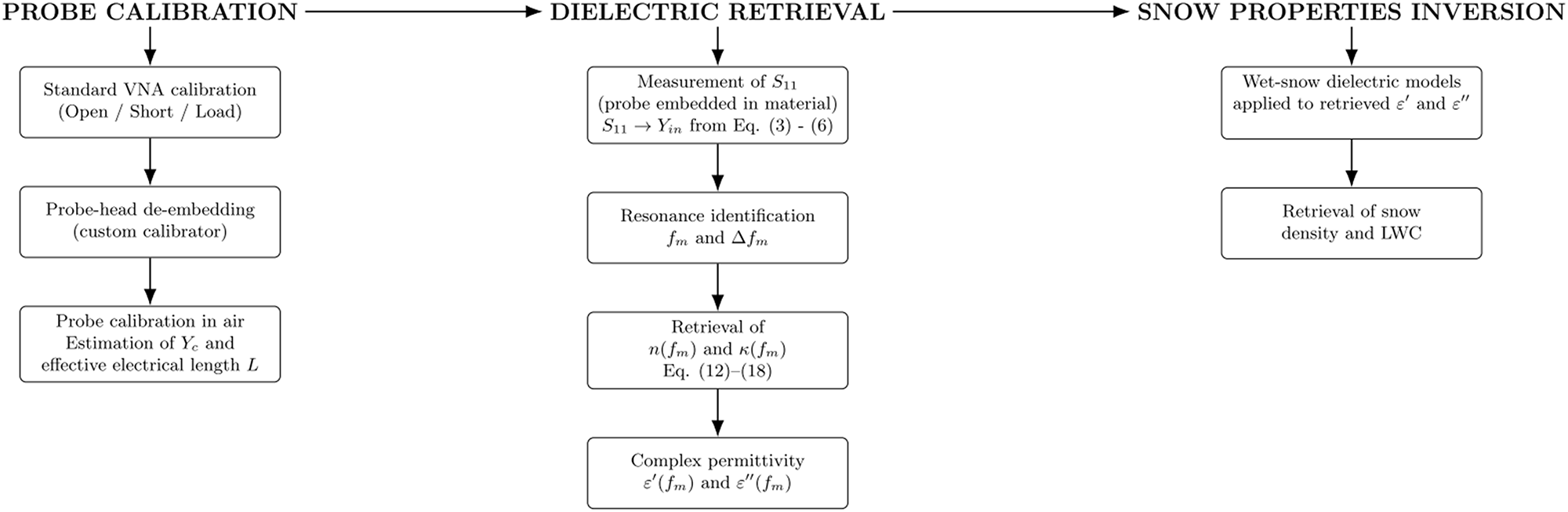


 Open access

