Role of Klebanoff modes in active flow control of separation: direct numerical simulations

Shirzad Hosseinverdi; Hermann F. Fasel

doi:10.1017/jfm.2018.489

Role of Klebanoff modes in active flow control of separation: direct numerical simulations

Published online by Cambridge University Press: 10 July 2018

Shirzad Hosseinverdi

and

Hermann F. Fasel

Show author details

Shirzad Hosseinverdi*: Affiliation:
Department of Aerospace and Mechanical Engineering, University of Arizona, Tucson, AZ 85721, USA
Hermann F. Fasel: Affiliation:
Department of Aerospace and Mechanical Engineering, University of Arizona, Tucson, AZ 85721, USA
*: †Email address for correspondence: shirzadh@email.arizona.edu

Article contents

Abstract
Introduction
Computational framework
Results
Conclusion
References

Rights & Permissions

Abstract

Our previous research has shown that an active flow control strategy using two-dimensional (2-D) harmonic blowing and suction with properly chosen frequency and amplitude can significantly reduce the separation region, delay transition to turbulence and can even relaminarize the flow. How such effective flow control for transition delay and relaminarization is affected by free-stream turbulence (FST) remains an open question. In order to answer this question, highly resolved direct numerical simulations (DNS) are carried out where very low-amplitude isotropic FST fluctuations are introduced at the inflow boundary of the computational domain. With FST the effectiveness of the flow control is not diminished, and the extent of the separated flow region is reduced by the same amount as for the zero FST case. However, a striking difference observed in the DNS is the fact that in the presence of even very low levels of FST, the flow transitions shortly downstream of the reattachment location of the bubble, contrary to the case without FST. It appears that this different behaviour for even very small levels of FST is caused by an interaction between the high-amplitude 2-D disturbances introduced by the flow control forcing and 3-D Klebanoff modes (K-modes) that are generated by the FST. The streamwise elongated streaks due to the K-modes cause a spanwise-periodic modulation of the basic flow and subsequently of the primary 2-D wave. The disturbances associated with this modulation exhibit strong growth and initiate the breakdown process to turbulence. Linear secondary instability investigations with respect to low-frequency 3-D disturbances are carried out based on the linearized Navier–Stokes equations. The response of the forced flow to the low-frequency 3-D disturbances reveals that the time-periodic base flow is unstable with respect to a wide range of 3-D modes. In particular, the wavelength associated with the spanwise spacing of the K-mode falls into the range of, and is in fact very close to, the most unstable 3-D disturbances. Results from the secondary instability analysis and the comparison with DNS results, support the conjecture that the forcing amplitude has a major impact on the onset and amplification rate of the K-modes: lowering the forcing amplitude postpones the onset of the growth of the K-modes and reduces the growth rate of the K-modes for a given FST intensity. The net effect of these two events is a delay of the transition onset. Nevertheless, the instability mechanism that governs the transition process is the same as previously identified, i.e. interaction of the K-mode and 2-D primary wave. Furthermore, for low levels of FST, the amplitude of the low-frequency K-modes scales linearly with the FST intensity in the approach boundary layer up to the secondary instability regime.

JFM classification

Boundary Layers: Boundary layer separation Flow Control: Flow Control Instability: Transition to turbulence

Information

Type: JFM Papers
Information: Journal of Fluid Mechanics , Volume 850 , 10 September 2018, pp. 954 - 983
DOI: https://doi.org/10.1017/jfm.2018.489 [Opens in a new window]
Copyright: © 2018 Cambridge University Press

1 Introduction

For flight vehicles, successful active flow control (AFC) strategies to mitigate the detrimental effects of boundary-layer separation for lifting surfaces could lead to significant performance gains. This is especially true for unmanned aerial vehicles (UAVs) which, due to the usually small wing dimensions and low air speeds, often operate within a Reynolds-number flight regime, for which a strong interaction exists between separation and transition. Hydrodynamic instabilities and the laminar-to-turbulent transition process have a profound impact on the mean flow topology and the unsteady behaviour of unforced/forced laminar separation bubbles (LSBs). Therefore, an improved understanding of the relevant physical mechanisms governing separation and separation control in general, and the transition process in particular, especially in the presence of free-stream turbulence, is required.

The laminar–turbulent transition process in boundary layers can be understood as a progression of stages, which depend on many parameters, such as Reynolds number, pressure gradient, environmental disturbances, etc. (Morkovin, Reshotko & Herbert Reference Morkovin, Reshotko and Herbert1994). In the framework of spatially growing perturbations in ‘quiet’ free-stream disturbance environments, which are typical of flight conditions, the transition process can be broken down into four major stages (according to Morkovin et al. Reference Morkovin, Reshotko and Herbert1994): receptivity, linear ‘eigenmode’ growth, secondary instability and nonlinear breakdown. Receptivity in the present context refers to the process through which external disturbances (such as free-stream turbulence, acoustic waves or surface roughness, etc.) penetrate the boundary layer and generate instability modes such as the Tollmien–Schlichting (TS) waves. For a zero-pressure-gradient (ZPG) flat-plate boundary layer, transition can be initiated by the exponential growth of TS waves when the critical Reynolds number, $Re_{cr}$ , is exceeded. An adverse pressure gradient (APG) has a destabilizing effect, effectively decreasing the critical Reynolds number. If the adverse pressure gradient is strong enough, the flow separates: the resulting velocity profile in the separated region becomes inviscidly unstable (often referred to as Kelvin–Helmholtz instability) due to the presence of an inflection point in the velocity profile. The switchover from the viscous TS instability mechanism in the approaching attached boundary layer to the inviscid Kelvin–Helmholtz (KH) instability leads to growth rates that are much larger compared to the growth rates associated with TS instabilities for the attached boundary layer. As a result, high-frequency, two-dimensional or weakly oblique disturbances can rapidly reach large (nonlinear) amplitudes within the separated region, leading to the commonly observed periodic shedding of spanwise coherent vortical structures that are often referred to as ‘rollers’. At this stage, secondary instabilities can take hold, which subsequently leads to a rapid breakdown to small-scale three-dimensional (3-D) structures and eventually to a fully turbulent flow (see Marxen et al. Reference Marxen, Lang, Rist and Wagner2003; Diwan & Ramesh Reference Diwan and Ramesh2009; Marxen & Henningson Reference Marxen and Henningson2011; Marxen, Lang & Rist Reference Marxen, Lang and Rist2012; Balzer & Fasel Reference Balzer and Fasel2016).

Previous studies have shown that active flow control that exploits the shear-layer instability is both effective and efficient for controlling laminar separation bubble at low Reynolds numbers (Jones, Sandberg & Sandham Reference Jones, Sandberg and Sandham2008; Postl, Balzer & Fasel Reference Postl, Balzer and Fasel2011; Embacher & Fasel Reference Embacher and Fasel2014; Benton & Visbal Reference Benton and Visbal2016). The primary convective instability strongly amplifies the disturbance waves (within the Kelvin–Helmholtz frequency range of the separated shear layer), that are introduced upstream of the separation location, until they saturate to finite nonlinear amplitudes, leading to the commonly observed periodic shedding of spanwise coherent vortical structures. The presence of the large-amplitude waves (or vortices) facilitates an exchange of momentum, which limits the extent of the separation region.

The onset of unsteadiness in LSBs must not necessarily be caused by the spatial growth of incoming disturbances (convective instability) as observed by Spalart & Strelets (Reference Spalart and Strelets2000) and Jones et al. (Reference Jones, Sandberg and Sandham2008). Besides the ‘amplifier characteristics’ of the LSBs, Huerre & Monkewitz (Reference Huerre and Monkewitz1990) showed that LSBs can also act as oscillators where the disturbance waves propagate in both the downstream and upstream directions while being amplified in time, independent of external excitations, and ultimately result in vortex shedding leading to transition. This type of instability, which is not limited to separated flows, is called ‘absolute/global instability’. For a separation bubble, two parameters play an important role in the context of absolute instability: (i) the height of the bubble and (ii) the magnitude of the reverse flow (Rodríguez & Theofilis Reference Rodríguez and Theofilis2010). In general, a reverse flow of approximately 7–10 % of the free-stream velocity is required for the onset of an absolute instability. Rodríguez, Gennaro & Juniper (Reference Rodríguez, Gennaro and Juniper2013) demonstrated that the nature of such an instability mode is a global centrifugal instability, which requires a reverse flow with a magnitude of 7–8 % of the free-stream velocity.

In addition to reducing the extent of the separated flow region, Embacher & Fasel (Reference Embacher and Fasel2014) have shown that high-amplitude 2-D disturbance waves with a properly chosen frequency and amplitude can suppress the secondary absolute instability and thus delay transition and even relaminarize the flow downstream of reattachment. In these high-order accurate numerical simulations, the effects of realistic operation conditions, such as free-stream turbulence, noise and vibrations were neglected. Therefore, the question arises whether the observed transition delay and relaminarization of the flow is still possible in a ‘real’ environment as encountered in free flight or wind/water tunnel experiments.

From experiments (Klebanoff Reference Klebanoff1971; Kendall Reference Kendall1985, Reference Kendall1990), theoretical and numerical studies (Leib, Wundrow & Goldstein Reference Leib, Wundrow and Goldstein1999; Ricco, Luo & Wu Reference Ricco, Luo and Wu2011; Goldstein Reference Goldstein2014) and direct numerical simulations (Jacobs & Durbin Reference Jacobs and Durbin2001; Brandt, Schlatter & Henningson Reference Brandt, Schlatter and Henningson2004; Balzer & Fasel Reference Balzer and Fasel2016), it is well known that free-stream turbulence (FST) can cause the formation of streamwise elongated streaks inside the laminar boundary layer, the so-called Klebanoff modes (K-modes). The K-mode is manifested in the form of a significant distortion in the u-velocity component in the spanwise and wall-normal directions. K-modes are fundamentally different from Tollmien–Schlichting waves. Characteristic features of the K-mode are its low frequency, low spatial growth rate and spanwise length scale of a few boundary-layer thicknesses.

The interaction of TS waves and streamwise streaks (or K-modes) in a ZPG boundary layer has been investigated using numerical simulations (Fasel Reference Fasel2002; Liu, Zaki & Durbin Reference Liu, Zaki and Durbin2008a ), secondary stability analysis (Liu, Zaki & Durbin Reference Liu, Zaki and Durbin2008b ) and experiments (Fransson et al. Reference Fransson, Brandt, Talamelli and Cossu2005). A key result was that, while streaks of large or small spanwise wavelengths reduce the growth rate of the primary TS waves, they can also enhance secondary instabilities by promoting the formation of $\unicode[STIX]{x1D6EC}$ vortices. Another important observation in the direct numerical simulations of Fasel (Reference Fasel2002) and Liu et al. (Reference Liu, Zaki and Durbin2008a ) was that the spanwise wavelengths of the $\unicode[STIX]{x1D6EC}$ -structures were related to the spanwise wavelength of the streaks, which is much smaller than the one obtained from classical secondary instability, i.e. fundamental and subharmonic resonances without the presence of streaks (Herbert Reference Herbert1988). Furthermore, secondary instability investigations using a Floquet analysis of a ZPG boundary layer distorted by Klebanoff modes and (saturated) TS waves by Liu et al. (Reference Liu, Zaki and Durbin2008b ) predicted that the ‘wide’ streaks ( $\unicode[STIX]{x1D6FD}\unicode[STIX]{x1D6FF}_{1}=0.54$ ) promote both fundamental and subharmonic secondary instabilities ( $\unicode[STIX]{x1D6FD}$ and $\unicode[STIX]{x1D6FF}_{1}$ correspond to the spanwise wavelength and displacement thickness, respectively). In contrast, for the ‘narrow’ streak case ( $\unicode[STIX]{x1D6FD}\unicode[STIX]{x1D6FF}_{1}=1.35$ ), the secondary instability is dominated by a detuned instability.

For airplane applications, it is reasonable to assume that surface roughness and free-stream turbulence can provide the disturbances that influence laminar–turbulent transition. Both have to be considered when investigating separation and separation control. The main objective of the present numerical investigations is to gain insight into the underlying physical mechanisms governing active flow control applied to LSBs in the presence of low levels of free-stream turbulence. Towards this end, possible interactions of instability modes induced by FST and the disturbances introduced by the forcing applied for the control in a strong APG boundary layer are investigated. In particular, highly resolved direct numerical simulation (DNS) data are scrutinized using instantaneous flow visualizations, spectral analysis, proper orthogonal decomposition and secondary instability analysis (SIA) with the goal of understanding whether FST affects the surprising effectiveness of 2-D harmonic excitation for transition delay and relaminarization as found by Embacher & Fasel (Reference Embacher and Fasel2014). Towards this end, very low-amplitude isotropic FST velocity and vorticity fluctuations are introduced at the inflow boundary of the computational domain and a response of separated flow to the forcing in the presence of FST is investigated. Our main focus in this paper will be on low levels of FST, as this is more relevant for free flight and high-quality water/wind tunnel experiments. Furthermore, a main focus is on controlled LSBs where relaminarization and transition delay is achievable in the absence of FST.

The paper is organized as follows: in the next section, § 2, the computational set-up, the free-stream turbulence generation and disturbance generation for the flow control are introduced. A detailed discussion of the results is provided in § 3. A summary of the results and the contributions of the paper are given in § 4.

2 Computational framework

An extensively validated high-order accurate Navier–Stokes solver developed in our Computational Fluid Dynamics (CFD) Laboratory was employed for the present numerical simulations (Meitz & Fasel Reference Meitz and Fasel2000). The simulation code solves the three-dimensional, unsteady incompressible Navier–Stokes equations in vorticity–velocity formulation

(2.1)

$$\begin{eqnarray}\displaystyle & \displaystyle {\displaystyle \frac{\unicode[STIX]{x2202}\unicode[STIX]{x1D74E}}{\unicode[STIX]{x2202}t}}=\unicode[STIX]{x1D735}\times (\boldsymbol{u}\times \unicode[STIX]{x1D74E})+{\displaystyle \frac{1}{Re}}\unicode[STIX]{x1D6FB}^{2}\unicode[STIX]{x1D74E}, & \displaystyle\end{eqnarray}$$

where the vorticity, $\unicode[STIX]{x1D74E}$ , is defined as the negative curl of the velocity $\unicode[STIX]{x1D74E}=-\unicode[STIX]{x1D735}\times \boldsymbol{u}$ . In the above equation, the global Reynolds number is defined as $Re=U_{\infty }^{\ast }L_{\infty }^{\ast }/\unicode[STIX]{x1D708}^{\ast }$ , where $U_{\infty }^{\ast }$ and $L_{\infty }^{\ast }$ are reference velocity and length scales, respectively, and $\unicode[STIX]{x1D708}^{\ast }$ is the kinematic viscosity. The asterisk is used to denote dimensional quantities. Coordinates and velocities were made dimensionless with $L_{\infty }^{\ast }$ and $U_{\infty }^{\ast }$ , respectively.

With the definition of vorticity and using the fact that both the velocity and vorticity vector fields are solenoidal, the Poisson equations for the velocity components are obtained,

(2.2)

$$\begin{eqnarray}\displaystyle \unicode[STIX]{x1D6FB}^{2}\boldsymbol{u}=\unicode[STIX]{x1D735}\times \unicode[STIX]{x1D74E}. & & \displaystyle\end{eqnarray}$$

The governing equations are solved in a three-dimensional Cartesian coordinate system where the streamwise, wall-normal and spanwise directions are denoted by $x$ , $y$ and $z$ , respectively, and the corresponding velocity and vorticity components are denoted by ( $u$ , $v$ , $w$ ) and ( $\unicode[STIX]{x1D714}_{x}$ , $\unicode[STIX]{x1D714}_{y}$ , $\unicode[STIX]{x1D714}_{z}$ ), respectively.

The governing equations are integrated in time using an explicit fourth-order accurate Runge–Kutta scheme. All derivatives in the streamwise and wall-normal directions are approximated with fourth-order accurate compact differences. In the wall-normal direction, an exponential grid stretching is used in order to cluster grid points near the wall. Note that the finite difference approximations for the derivatives with respect to y are constructed for a non-equidistant grid instead of using a coordinate transformation. The flow field is assumed to be periodic in the spanwise direction. Therefore, the flow field is expanded in Fourier cosine and sine series with a pseudo-spectral treatment of the nonlinear terms. More details on the DNS code can be found in Meitz & Fasel (Reference Meitz and Fasel2000) and Balzer & Fasel (Reference Balzer and Fasel2016).

2.1 Simulation set-up

The computational domain for the DNS is the same as that used by Balzer & Fasel (Reference Balzer and Fasel2016) (see figure 4 in Balzer & Fasel Reference Balzer and Fasel2016) which was guided by the experimental investigations of laminar separation bubbles by Gaster (Reference Gaster1967), specifically series I case VI. In the experiments, laminar separation was generated on a flat plate through the close proximity of an auxiliary wing that is mounted inverted in the wind tunnel. This model geometry is designed such that it models a flow with similar physical properties as the flow over an airfoil but at reduced geometric complexity.

The velocity scale is chosen according to the tunnel speed in the experiments, $U_{\infty }^{\ast }=6.64~(\text{m}~\text{s}^{-1})$ . The reference length scale is $L_{\infty }^{\ast }=0.0254~(\text{m})$ . This length scale does not, however, correspond to a scale with physical meaning. It is chosen because the experimental data were reported in inches. The computational domain for the DNS is defined as $5\leqslant x\leqslant 19.4$ , $0\leqslant y\leqslant 2$ , and the domain width in the spanwise direction is $L_{z}=2$ . All the simulations presented in this work are carried out using the same computational grid with a resolution of $N_{x}\times N_{y}\times N_{z}=1801\times 300\times 250\approx 135$ million grid points. The grid spacing is uniform in the streamwise direction. The grid resolution in wall units, $\unicode[STIX]{x1D6E5}^{+}$ , within the separation bubble and in the redeveloping turbulent boundary layer downstream of the reattachment point is $\unicode[STIX]{x0394}x^{+}\leqslant 5.3$ , $\unicode[STIX]{x0394}z^{+}\leqslant 5.3$ and $\unicode[STIX]{x0394}y_{w}^{+}\leqslant 0.5$ , where $\unicode[STIX]{x1D6E5}^{+}$ is calculated according to $\unicode[STIX]{x1D6E5}^{+}=Re\sqrt{c_{f}/2}\unicode[STIX]{x1D6E5}$ . The grid resolution in the presented simulations is slightly finer compared to the resolutions used in Balzer & Fasel (Reference Balzer and Fasel2016).

At the inflow boundary all velocity and vorticity components are specified. Specifically, the velocity and vorticity components of a two-dimensional (2-D) steady-state basic flow (obtained from the Blasius solution) and superposing the velocity and vorticity fluctuations from the FST model, are prescribed as Dirichlet conditions. The displacement thickness Reynolds number at the inflow is $Re_{\unicode[STIX]{x1D6FF}_{1}}=407.8$ . In addition, for maintaining the fourth-order accuracy of the code near the inflow boundary, the streamwise derivatives of all dependent variables are prescribed as well.

A v-velocity distribution is applied as a Dirichlet boundary condition at the upper boundary for generating the favourable to adverse pressure gradients that induce laminar separation on the flat plate. It is chosen such that the resulting downstream pressure gradient closely matches that of the wind tunnel experiments by Gaster (Reference Gaster1967). More details and validation regarding the free-stream boundary condition can be found in Balzer & Fasel (Reference Balzer and Fasel2016).

At the outflow boundary, all second derivatives in the streamwise direction are set to zero. In addition, a buffer domain in region $18.1\leqslant x\leqslant 19.4$ , as proposed by Meitz & Fasel (Reference Meitz and Fasel2000), is employed in order to smoothly dampen out the fluctuations generated inside the domain and to prevent upstream contamination.

2.2 Free-stream turbulence generation

The methodology adopted here to generate free-stream disturbances at the inflow boundary of the computational domain is similar to that proposed by Jacobs & Durbin (Reference Jacobs and Durbin2001) and Brandt et al. (Reference Brandt, Schlatter and Henningson2004) i.e. a superposition of eigenmodes from the continuous spectra of the Orr–Sommerfeld (OS) and homogeneous Squire (SQ) operators

(2.3)

$$\begin{eqnarray}\displaystyle & \displaystyle \boldsymbol{u}^{\prime }(x_{0},y,z,t)=\mathop{\sum }_{\unicode[STIX]{x1D714}}\mathop{\sum }_{k_{z}}\mathop{\sum }_{k_{y}}A(k)\unicode[STIX]{x1D731}(y;\unicode[STIX]{x1D714},k_{y},k_{z})\text{e}^{\text{i}(k_{z}z-\unicode[STIX]{x1D714}t)}, & \displaystyle\end{eqnarray}$$

where $\unicode[STIX]{x1D714}$ is the angular disturbance frequency, $k_{y}$ and $k_{z}$ are the wall-normal and spanwise wavenumbers, respectively with $k=(\unicode[STIX]{x1D714}^{2}+k_{y}^{2}+k_{z}^{2})^{0.5}$ . The dispersion relation $k_{x}=\unicode[STIX]{x1D714}/U_{\infty }$ was used in (2.3) to express the streamwise wavenumber in terms of the angular frequency. In the same manner, the inflow disturbance vorticity field is calculated from the disturbance velocity field as $\unicode[STIX]{x1D74E}^{\prime }=-\unicode[STIX]{x1D6FB}\times \boldsymbol{u}^{\prime }$ . The coefficients $A(k)$ determine the contribution of the eigenfunctions to the total turbulent kinetic energy. The eigenfunction $\unicode[STIX]{x1D731}$ is a normalized weighted superposition of OS and SQ eigenmodes as follows

(2.4)

$$\begin{eqnarray}\displaystyle \unicode[STIX]{x1D731}=[\unicode[STIX]{x1D6F7}_{u},\unicode[STIX]{x1D6F7}_{v},\unicode[STIX]{x1D6F7}_{w}]^{T}={\displaystyle \frac{1}{E_{\unicode[STIX]{x1D731}}}}[\text{e}^{\text{i}\unicode[STIX]{x1D703}_{1}}\cos (\unicode[STIX]{x1D719})\unicode[STIX]{x1D731}_{OS}+\text{e}^{\text{i}\unicode[STIX]{x1D703}_{2}}\sin (\unicode[STIX]{x1D719})\unicode[STIX]{x1D731}_{SQ}]^{\text{T}}. & & \displaystyle\end{eqnarray}$$

Here $\unicode[STIX]{x1D703}_{1}$ , $\unicode[STIX]{x1D703}_{2}$ and $\unicode[STIX]{x1D719}$ are uniformly distributed random numbers, and $\unicode[STIX]{x1D731}_{OS}$ and $\unicode[STIX]{x1D731}_{SQ}$ represent the OS and SQ continuous modes. The normalization is such that the energy of each disturbance mode is 1. This leads to an expression for $E_{\unicode[STIX]{x1D731}}$ :

(2.5)

$$\begin{eqnarray}\displaystyle & \displaystyle E_{\unicode[STIX]{x1D731}}={\displaystyle \frac{1}{y_{max}}}\int _{0}^{y_{max}}{\displaystyle \frac{1}{2}}(\unicode[STIX]{x1D6F7}_{u}\unicode[STIX]{x1D6F7}_{u}^{\ast }+\unicode[STIX]{x1D6F7}_{v}\unicode[STIX]{x1D6F7}_{v}^{\ast }+\unicode[STIX]{x1D6F7}_{w}\unicode[STIX]{x1D6F7}_{w}^{\ast })\,\text{d}y. & \displaystyle\end{eqnarray}$$

The complex conjugate is denoted by the asterisk. The velocity fluctuations at the inflow model the specified energy spectrum. Various analytic forms for the energy spectrum exist. For the simulations presented in this work, the von Kármán energy spectrum is employed for distributing the turbulent kinetic energy among the various modes,

(2.6)

$$\begin{eqnarray}\displaystyle E(k)=Tu^{2}L_{11}{\displaystyle \frac{1.196(kL_{11})^{4}}{0.558[1+(kL_{11})^{2}]^{17/6}}}. & & \displaystyle\end{eqnarray}$$

The turbulent integral length scale, $L_{11}$ , determines the wavenumber associated with the maximum in the $E(k)$ distribution and Tu is the FST intensity. For large scales (small $k$ ) the spectrum is asymptotically proportional to $k^{4}$ . For small scales (large $k$ ) the spectrum matches Kolmogorov’s $k^{-5/3}$ law.

To obtain isotropic turbulence, several wavenumbers $k$ have to be selected in the domain $k_{min}\leqslant k\leqslant k_{max}$ , where the limiting wavenumbers are determined by the domain size and the computational resolution. For the present simulations, $k_{min}=2$ and $k_{max}=100$ was chosen. It is worth noting that the smallest and largest spanwise wavenumbers which are resolved by the DNS are $k_{z,min}=2.09$ and $k_{z,max}=131.95$ . For the present investigations, the wavenumber space ( $k$ ) was divided into 40 equidistant concentric spherical shells. Modes on a given shell have an identical wavenumber magnitude $k$ and a limited number, $N_{p}$ , of disturbance modes then selected on each shell where to each mode a wave vector $\boldsymbol{k}=[\unicode[STIX]{x1D714},k_{y},k_{z}]^{\text{T}}$ is associated such that $k=|\boldsymbol{k}|$ . After choosing the angular frequency, wall-normal and spanwise wavenumbers, the eigenvalue $\unicode[STIX]{x1D6FC}$ of the continuous spectrum can be obtained from analytical expression (see Grosch & Salwen Reference Grosch and Salwen1978; Jacobs & Durbin Reference Jacobs and Durbin2001) and then, the associated eigenmodes are obtained from the numerical solution of the homogenous OS/SQ system together with proper boundary conditions (see Brandt, Henningson & Ponziani Reference Brandt, Henningson and Ponziani2002). The coefficients of each terms in (2.3) are given by $A(k)=\sqrt{2E(k)\unicode[STIX]{x0394}k/N_{p}}$ , where $\unicode[STIX]{x0394}k$ is the difference in wavenumber between two shells. Finally, upon choosing the parameters $L_{11}$ and $Tu$ , the inflow velocity and vorticity disturbance fields can be entirely determined. In summary, the approach adopted in this paper to generate free-stream fluctuations is very similar to the procedure presented by Brandt et al. (Reference Brandt, Schlatter and Henningson2004).

It is worth noting that this approach using the homogenous SQ operator and a weighted superposition of eigenfunctions to generate inlet perturbations, avoids ‘abnormal anisotropy’ behaviour with respect to streamwise velocity in the coupled OS and SQ (inhomogeneous) system as pointed out by Dong & Wu (Reference Dong and Wu2013) and Wu & Dong (Reference Wu and Dong2016). Furthermore, the evolution of the disturbances downstream of the inflow boundary of the computational domain is computed by the complete Navier–Stokes equations and therefore non-parallel and nonlinear effects are fully taken into account.

For the present investigation, the turbulent integral length scale was chosen as $L_{11}=5\unicode[STIX]{x1D6FF}_{1,0}$ which is the same $L_{11}$ used in Balzer & Fasel (Reference Balzer and Fasel2016). Here $\unicode[STIX]{x1D6FF}_{1,0}$ is the displacement thickness at the inflow boundary. A detailed description of the implementation and validation results are provided in Hosseinverdi, Balzer & Fasel (Reference Hosseinverdi, Balzer and Fasel2012) and Balzer & Fasel (Reference Balzer and Fasel2016).

2.3 Flow control: harmonic blowing and suction through a 2-D slot

In the present simulation, high-amplitude, two-dimensional disturbance waves are generated upstream of the separation location by specifying a wall-normal velocity component across a narrow blowing and suction slot at the wall. The forcing function for the harmonic blowing and suction (HBS) simulations has the form

(2.7)

$$\begin{eqnarray}\displaystyle & \displaystyle v_{f}(x,t)=B\cdot S(x)\cdot \sin (2\unicode[STIX]{x03C0}f_{hbs}t), & \displaystyle\end{eqnarray}$$

where $B$ is the maximum forcing amplitude and $f_{hbs}$ represents the forcing frequency. The shape function, $S(x)$ , is a polynomial which is zero outside the suction/blowing slot such that smooth derivatives near boundaries of the suction/blowing slot are obtained:

(2.8)

$$\begin{eqnarray}\displaystyle S(x)={\displaystyle \frac{1}{48}}\left\{\begin{array}{@{}ll@{}}+729\unicode[STIX]{x1D713}^{5}-1701\unicode[STIX]{x1D713}^{4}+972\unicode[STIX]{x1D713}^{3}, & \unicode[STIX]{x1D713}={\displaystyle \frac{x-x_{s}}{x_{f}-x_{s}}};\quad x_{s}\leqslant x\leqslant x_{f},\\ -729\unicode[STIX]{x1D713}^{5}+1701\unicode[STIX]{x1D713}^{4}-972\unicode[STIX]{x1D713}^{3}, & \unicode[STIX]{x1D713}={\displaystyle \frac{x_{e}-x}{x_{e}-x_{f}}};\quad x_{f}\leqslant x\leqslant x_{e}.\end{array}\right. & & \displaystyle\end{eqnarray}$$

The downstream locations $x_{s}$ , $x_{e}$ and $x_{f}$ correspond the beginning, the end and the centre of the slot, respectively. This shape function guarantees zero net volume flux through the disturbance slot at any time instant.

3 Results

Results obtained from the 3-D DNS of the uncontrolled and controlled separation bubbles in the absence and presence of FST are discussed in this section. The main focus will be directed towards the response of a forced (‘controlled’) LSB to vortical perturbations generated by free-stream turbulence.

For the cases with forcing, 2-D disturbance waves were introduced upstream of the separation location at $x_{f}=9.5$ (the beginning of the adverse pressure gradient). The width of the forcing slot was 0.2. The frequency of the actuation is the same for the zero and non-zero FST cases and it is set to $f_{hbs}^{\ast }=240~(\text{hz})$ based on hydrodynamic results from instability analyses, see Hosseinverdi & Fasel (Reference Hosseinverdi and Fasel2017). The forcing frequency is very close to the natural shedding frequency of the unforced separation bubbles.

3.1 Main features of uncontrolled flow

Prior to the detailed discussion of the investigations for the controlled flow, results obtained from 3-D DNS for the uncontrolled case are presented in order to understand the relevant length scales of the LSBs in the presence and the absence of FST. For the simulation with FST, a full spectrum of isotropic FST with an intensity of $Tu=0.005\,\%$ is introduced at the inflow boundary of the computational domain as discussed above.

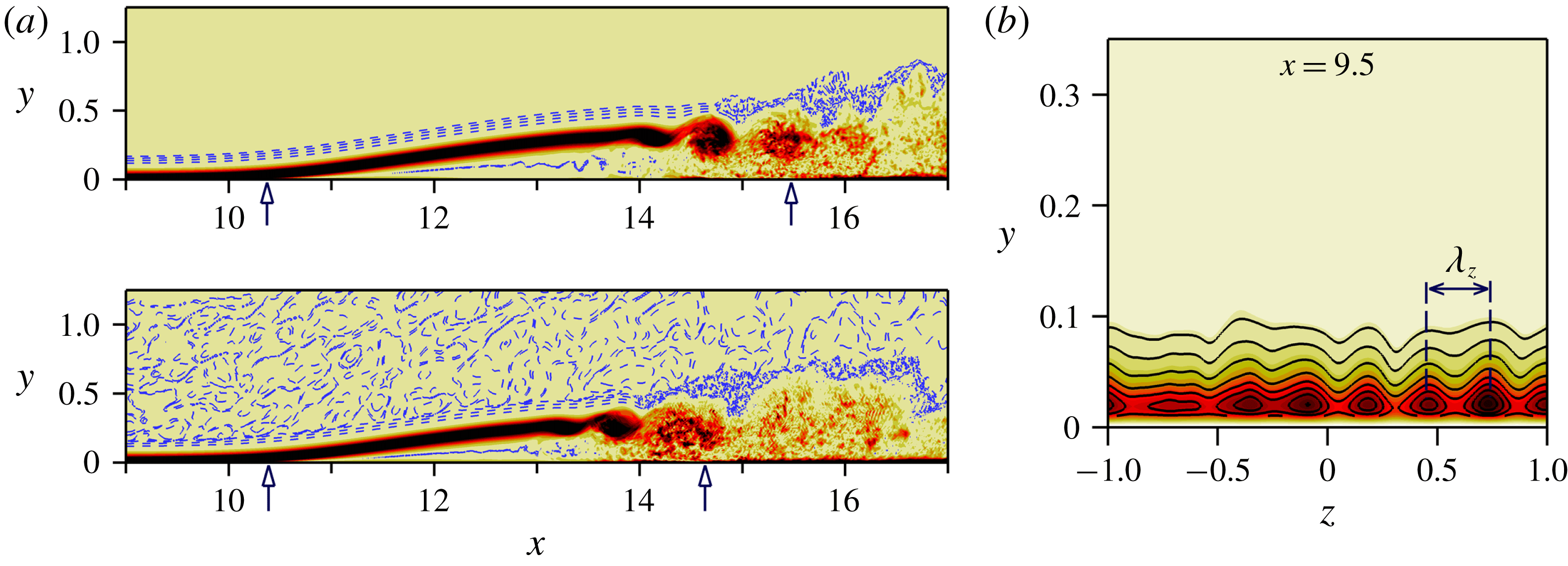
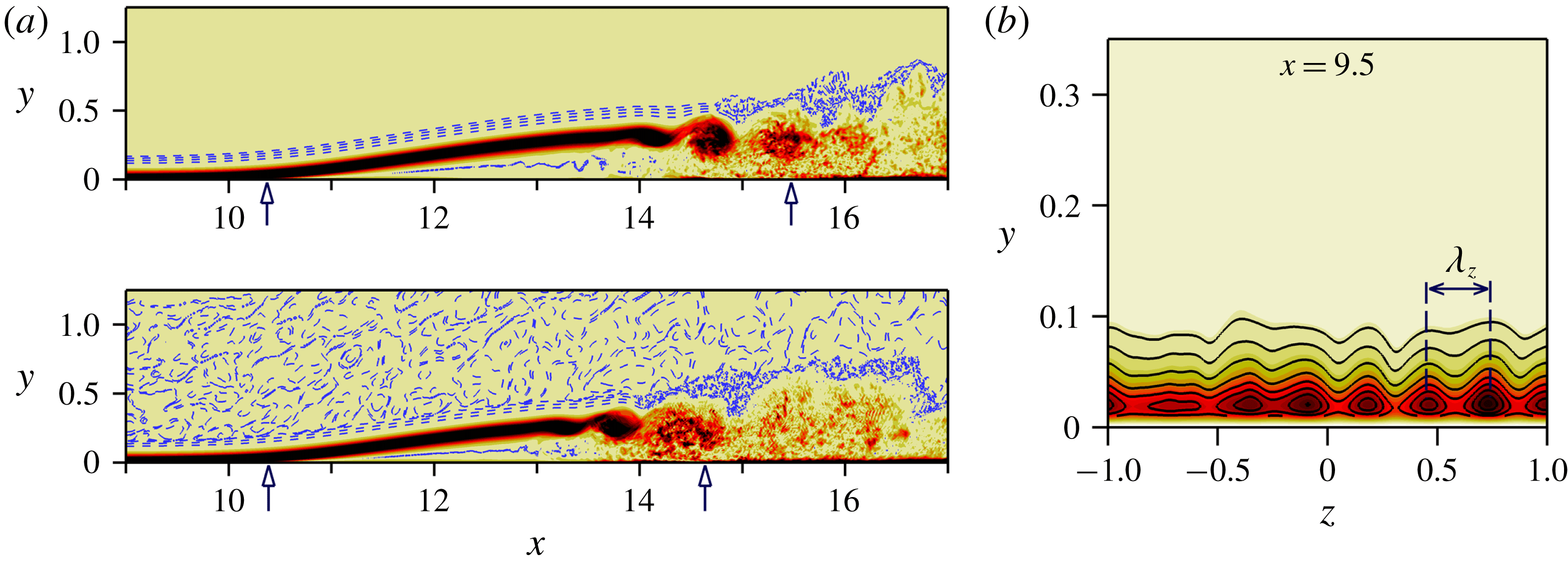
Instantaneous contours of spanwise vorticity, $\unicode[STIX]{x1D714}_{z}$ , of the uncontrolled flow for the two cases, $Tu=0$ and $Tu=0.005\,\%$ , are presented in figure 1(a) together with the contour lines of $\text{ln}|\unicode[STIX]{x1D714}_{z}|$ . A logarithmic scale was employed because the vorticity associated with the FST fluctuations in the free stream is much smaller than the vorticity associated with the near-wall structures for the case with FST. For the zero FST environment, the free stream is undisturbed (top plot). From the contours of $\unicode[STIX]{x1D714}_{z}$ -vorticity, it can be seen that the separated shear layer ‘rolls up’ and grows in intensity due to the Kelvin–Helmholtz instability as it is convected downstream. This is followed by shedding of strong spanwise coherent vortices (often referred to as ‘rollers’), finally leading to turbulent reattachment.

Hydrodynamic instability of laminar separated shear layers makes the LSB highly susceptive to the free-stream turbulence. Therefore, the onset of transition is moved upstream when the FST is introduced at the inflow, which in turn, leads to a slight reduction of the separated flow region. The free-stream vortical disturbances permeate into the boundary layer and induce low-frequency u-velocity distortions inside the laminar boundary layer – known as Klebanoff modes – as illustrated in figure 1(b) by the contours of $\overline{u^{\prime }u^{\prime }}$ at $x=9.5$ with a preferred spanwise wavelength of $\unicode[STIX]{x1D706}_{z}\approx L_{z}/7$ .

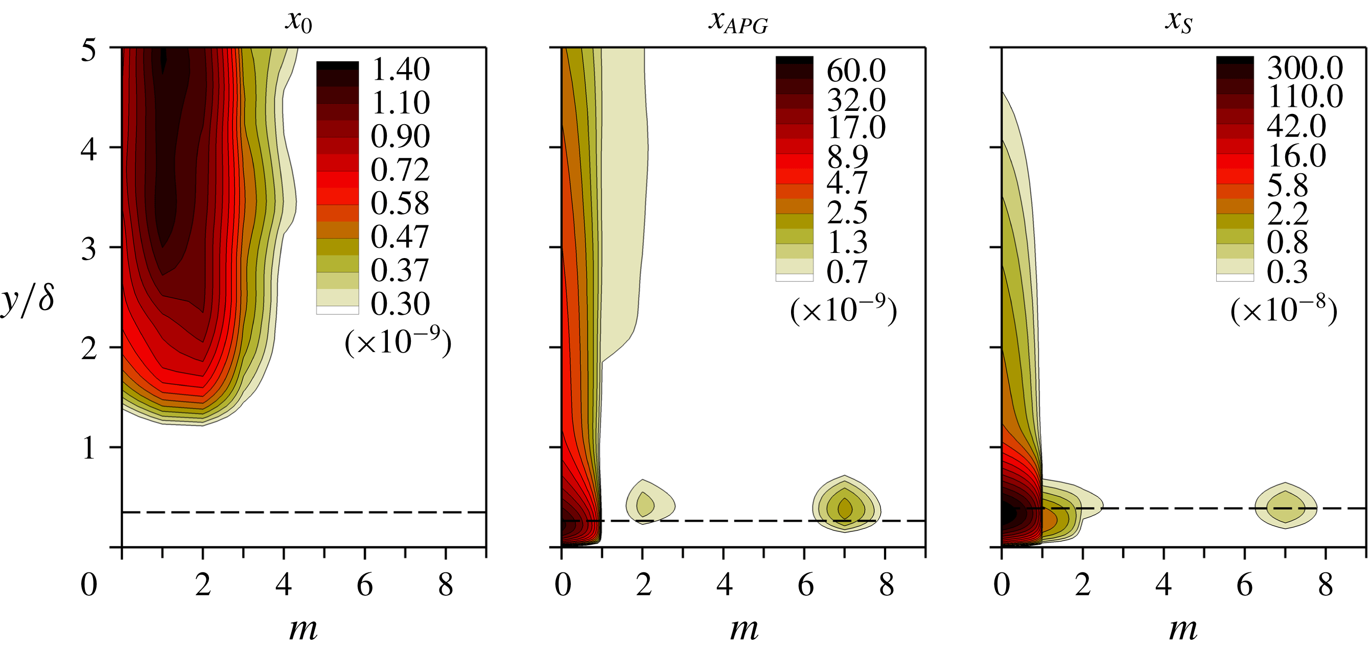
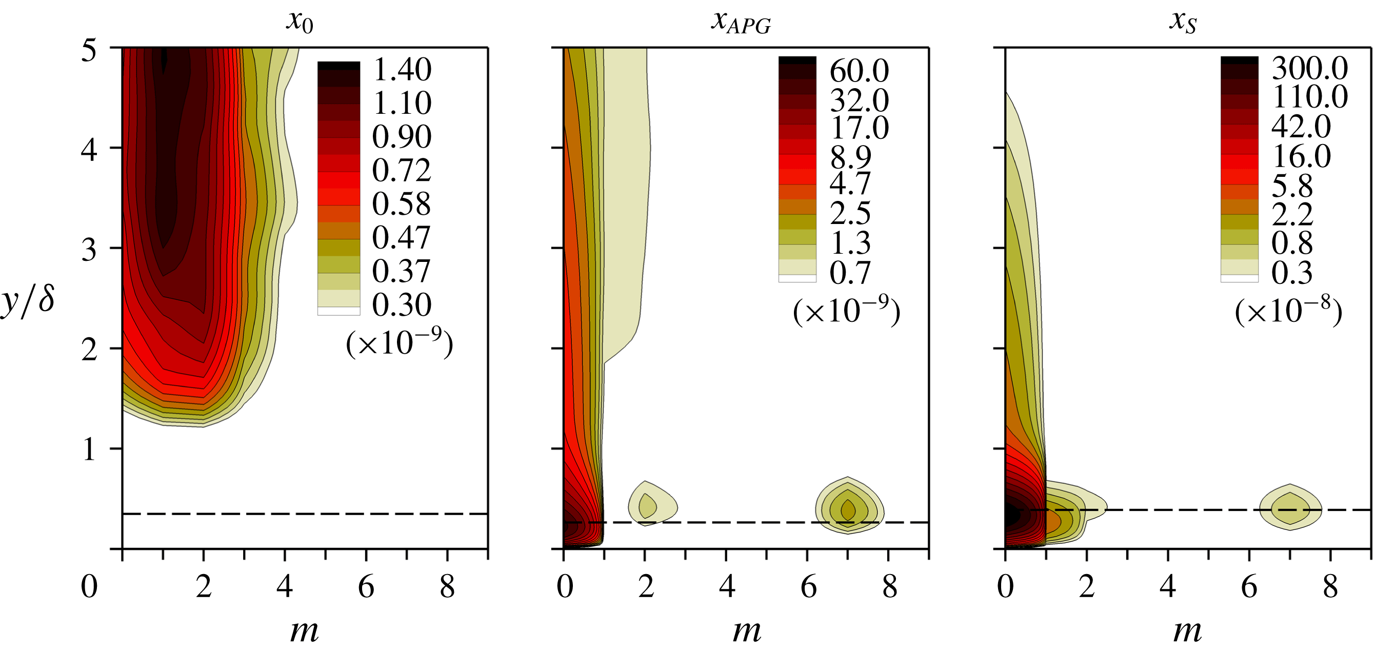
Contours of spanwise, one-dimensional power spectra of the $u^{\prime }$ -velocity as a function of the spanwise mode number $m$ ( $2\unicode[STIX]{x03C0}m/L_{z}$ is spanwise wavenumber) are plotted in figure 2 for selected streamwise locations for the uncontrolled case with FST. Three x-stations were selected: the inflow boundary, $x_{0}$ , the onset of the adverse pressure gradient, $x_{APG}$ , and the separation location, $x_{S}$ . The energy in the power spectrum at the inflow is clearly concentrated in the free stream and the maximum amplitude is at $1\leqslant m\leqslant 2$ (this is related to the chosen turbulent integral length scale $L_{11}$ ). While propagating in the downstream direction, the vortical structures in the free stream enter the boundary layer as can be clearly observed at $x_{APG}$ and $x_{S}$ . The disturbances with the spanwise mode number of $m=7$ correspond to the K-mode which is consistent with the figure 1(b) and also matches the finding of Balzer & Fasel (Reference Balzer and Fasel2016) for the spanwise spacing of K-mode. Furthermore, the spanwise spacing of the Klebanoff modes based on the local boundary-layer thickness, $\unicode[STIX]{x1D6FF}$ , is of the order of $\unicode[STIX]{x1D706}_{z,K}\approx (2.2\unicode[STIX]{x1D6FF}-3\unicode[STIX]{x1D6FF})$ for $9\leqslant x\leqslant x_{s}$ , which is consistent with the spanwise scaling of $O(2\unicode[STIX]{x1D6FF}-4\unicode[STIX]{x1D6FF})$ reported for ZPG flat-plate boundary layers (Kendall Reference Kendall1985, Reference Kendall1990).

Figure 1.

(a) Uncontrolled flow: instantaneous contours of $\unicode[STIX]{x1D714}_{z}$ -vorticity together with the contour lines of $\ln |\unicode[STIX]{x1D714}_{z}|$ for zero FST (top) and FST of $Tu=0.005\,\%$ (bottom). (b) Contours of the longitudinal component of the normal Reynolds stress, $\overline{u^{\prime }u^{\prime }}$ , at $x=9.5$ for $Tu=0.005\,\%$ . The overbar represents the time average. The mean separation and reattachment locations are marked by up arrows in (a).

Figure 2.

Spanwise one-dimensional energy spectra of the streamwise velocity at selected streamwise stations for the uncontrolled flow with $Tu=0.005\,\%$ . Dashed lines are the displacement thickness. The wall-normal coordinate was normalized with the local boundary-layer thickness.

Figure 3.

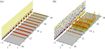
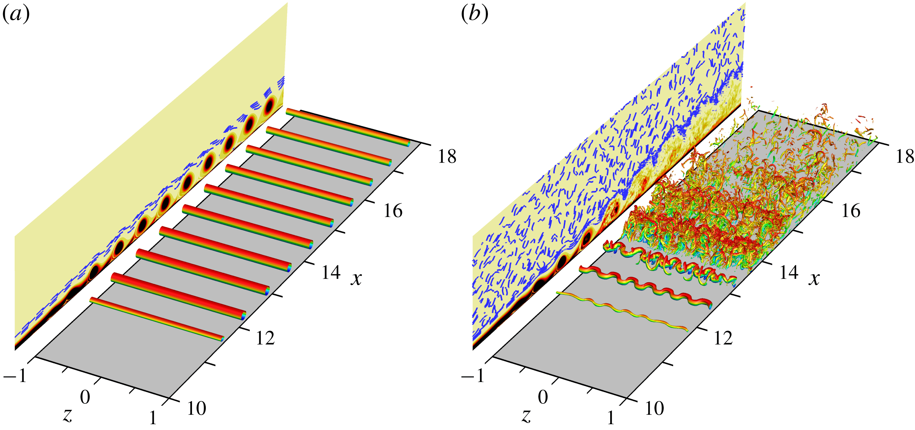
Instantaneous flow visualization for controlled flow. Plotted are iso-surfaces of $\unicode[STIX]{x1D706}_{2}=-40$ coloured by u-velocity in perspective view together with the contours of $\unicode[STIX]{x1D714}_{z}$ -vorticity and contour lines of $\ln |\unicode[STIX]{x1D714}_{z}|$ in the $x$ – $y$ plane (spanwise averaged). (a) zero FST; (b) $Tu=0.005\,\%$ .

3.2 Characteristic features of controlled flow

In this section, the response of the flow to the 2-D harmonic forcing with a wall-normal forcing amplitude of $B=0.05$ is discussed in detail for zero FST and a very low level of FST ( $Tu=0.005\,\%$ ).

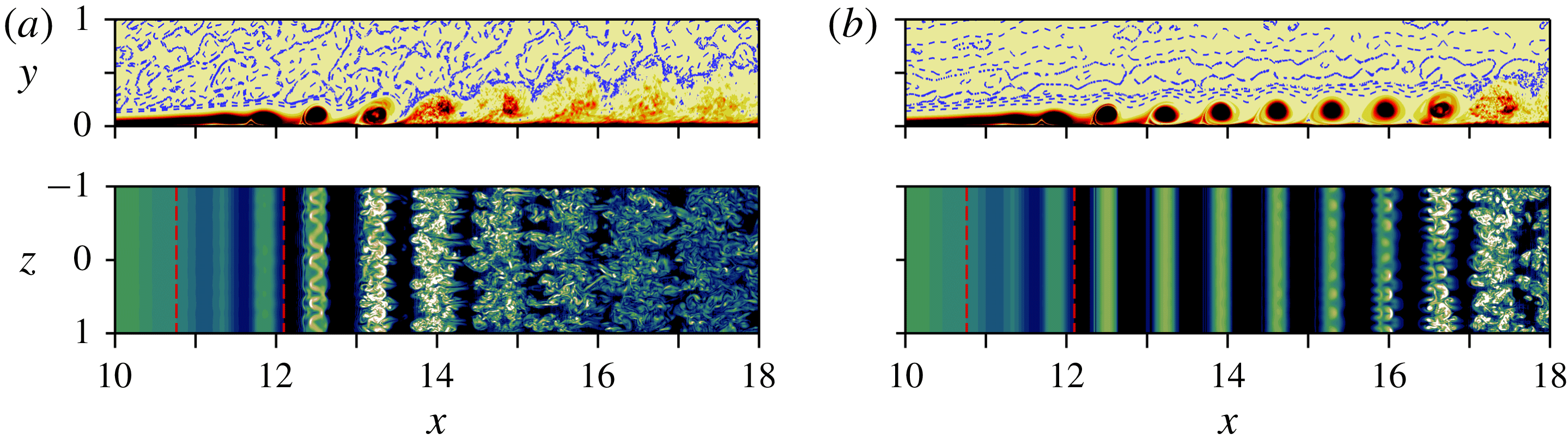
The effect of the forcing on the LSB is demonstrated in figure 3, which shows instantaneous perspective views of iso-surfaces of the $\unicode[STIX]{x1D706}_{2}$ -criterion coloured by the streamwise velocity together with the contours of the spanwise-averaged spanwise vorticity in the $x$ – $y$ plane. The visualizations for the zero FST case reveal that the flow is ‘locking on’ to the forcing signal and is shedding spanwise ‘rollers’ at the forcing frequency. The Kelvin–Helmholtz instability leads to the exponential growth of 2-D downstream travelling waves. At nonlinear saturation, these waves manifest themselves in form of spanwise ‘rollers’. These structures are very effective in increasing the wall-normal momentum transfer and therefore reducing the size of the separation bubble. Moreover, transition to turbulence is delayed significantly. In particular, transition does not occur within the integration domain and the flow remains completely laminar in the entire domain. The fact that for the controlled case the flow remains laminar far downstream suggests that the 2-D large-amplitude forcing is suppressing the secondary absolute instability. These findings are consistent with those by Embacher & Fasel (Reference Embacher and Fasel2014), who performed DNS for a similar separation bubble.

Spanwise rollers caused by strong forcing lead to a time-periodic base flow, thus, a secondary convective (possibly elliptical) instability is possible. In contrast to the zero FST case where 3-D disturbances have extremely low amplitude (‘numerical noise’) upstream of the separation location, the amplitude level of the 3-D disturbances is elevated in the presence of FST (orders of magnitude higher than in the zero FST case). As a result, the primary vortex cores appear modulated sinusoidally in the spanwise direction due to the secondary instability of the periodic controlled base flow as shown in figure 3(b). Contours of the spanwise-averaged spanwise vorticity (plotted in the $x$ – $y$ plane in figure 3 b) reveal that with FST the strong spanwise structures break up into smaller scales soon after their first appearance such that transition to turbulence is initiated immediately. In fact, prior to transition only three spanwise structures are still visible. The observed lateral wavelength of the modulation is identical to the spanwise spacing of the Klebanoff modes, i.e. $\unicode[STIX]{x1D706}_{z,K}=L_{z}/7$ . It is worth noting that the ratio of the spanwise wavelength to the streamwise wavelength of the disturbance waves in the transition region is $\unicode[STIX]{x1D706}_{z}/\unicode[STIX]{x1D706}_{x}\approx 0.41$ . A secondary stability analysis by von Terzi (Reference von Terzi2004) revealed that the most unstable spanwise wavelengths were in the range $0.3\leqslant \unicode[STIX]{x1D706}_{z}/\unicode[STIX]{x1D706}_{x}\leqslant 0.6$ for the separated shear layer developing behind a backward-facing step where a spanwise sinusoidal deformation of the primary vortices was observed similar to the present case.

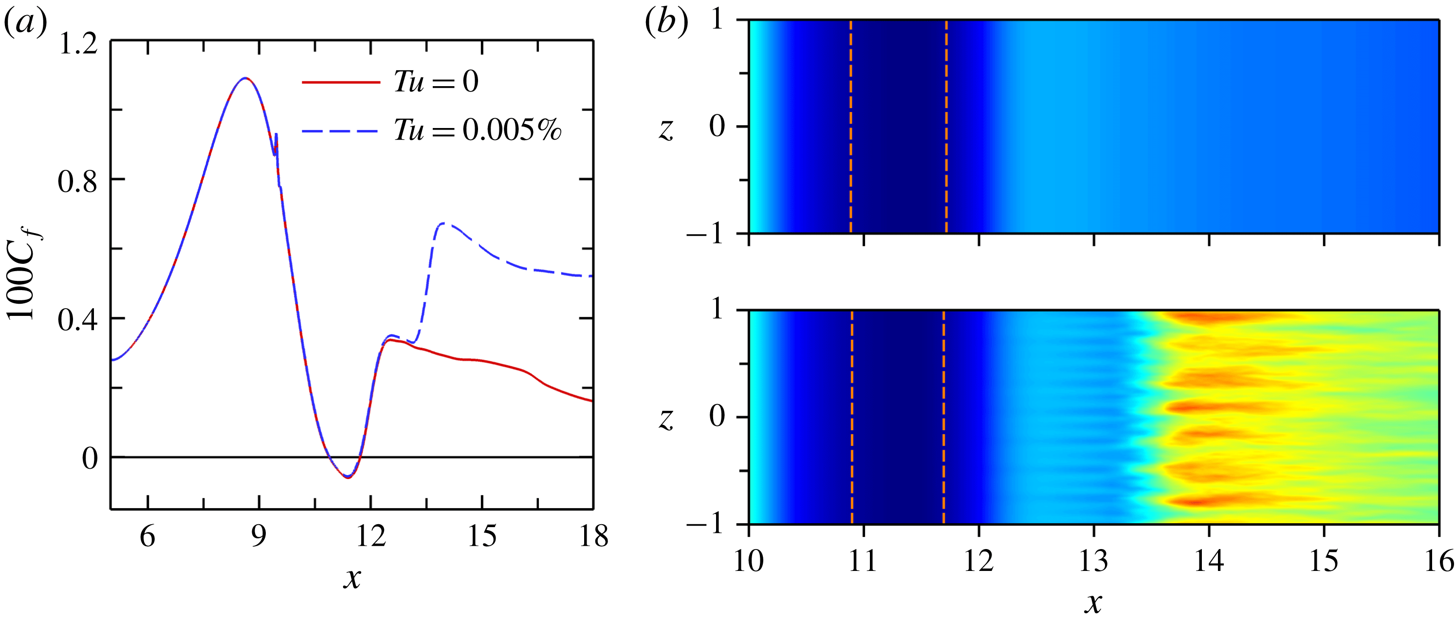
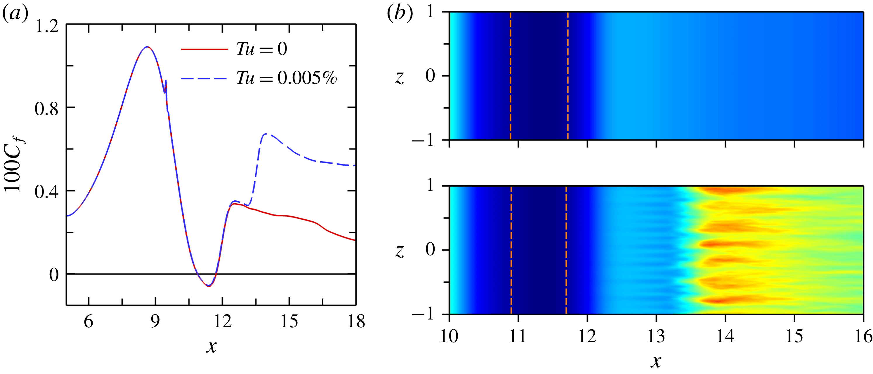
A comparison of the time- and spanwise-averaged skin-friction coefficient, $c_{f}$ , for the zero FST case and the FST case for the controlled flow is presented in figure 4(a). For a given forcing amplitude, the large 2-D vortices, whose strengths alone seems to determine the mean reattachment, leads to virtually identical bubble sizes independent of the FST. Figure 4(a) indicates that the value of $c_{f}$ for $Tu=0.005\,\%$ closely follows the laminar curve of the zero FST case until $x=13.2$ where it increases rapidly due to the laminar-to-turbulent transition. Time-averaged contours of $\unicode[STIX]{x1D714}_{z}$ -vorticity at the wall are plotted in figure 4(b). The $\unicode[STIX]{x1D714}_{z}$ -vorticity at the wall is directly proportional to the local skin friction. Also included are the $\overline{\unicode[STIX]{x1D714}}_{z}=0$ lines which indicate the time-mean separation and reattachment locations. Streamwise aligned ‘streaks’ are visible for $Tu=0.005\,\%$ downstream of the reattachment location, with a spanwise spacing that agrees very well with the spanwise spacing of the Klebanoff modes.

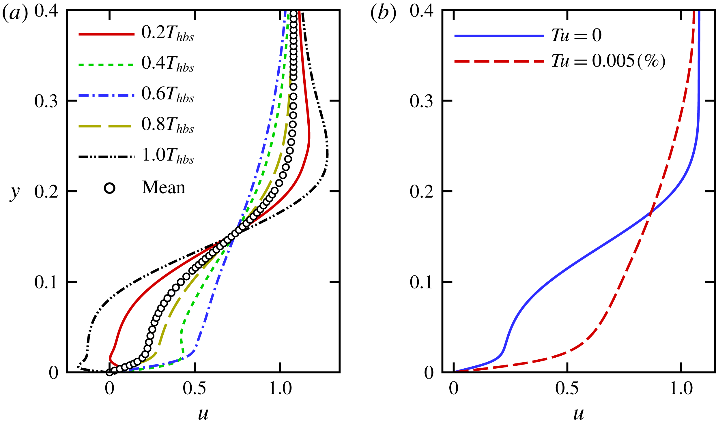
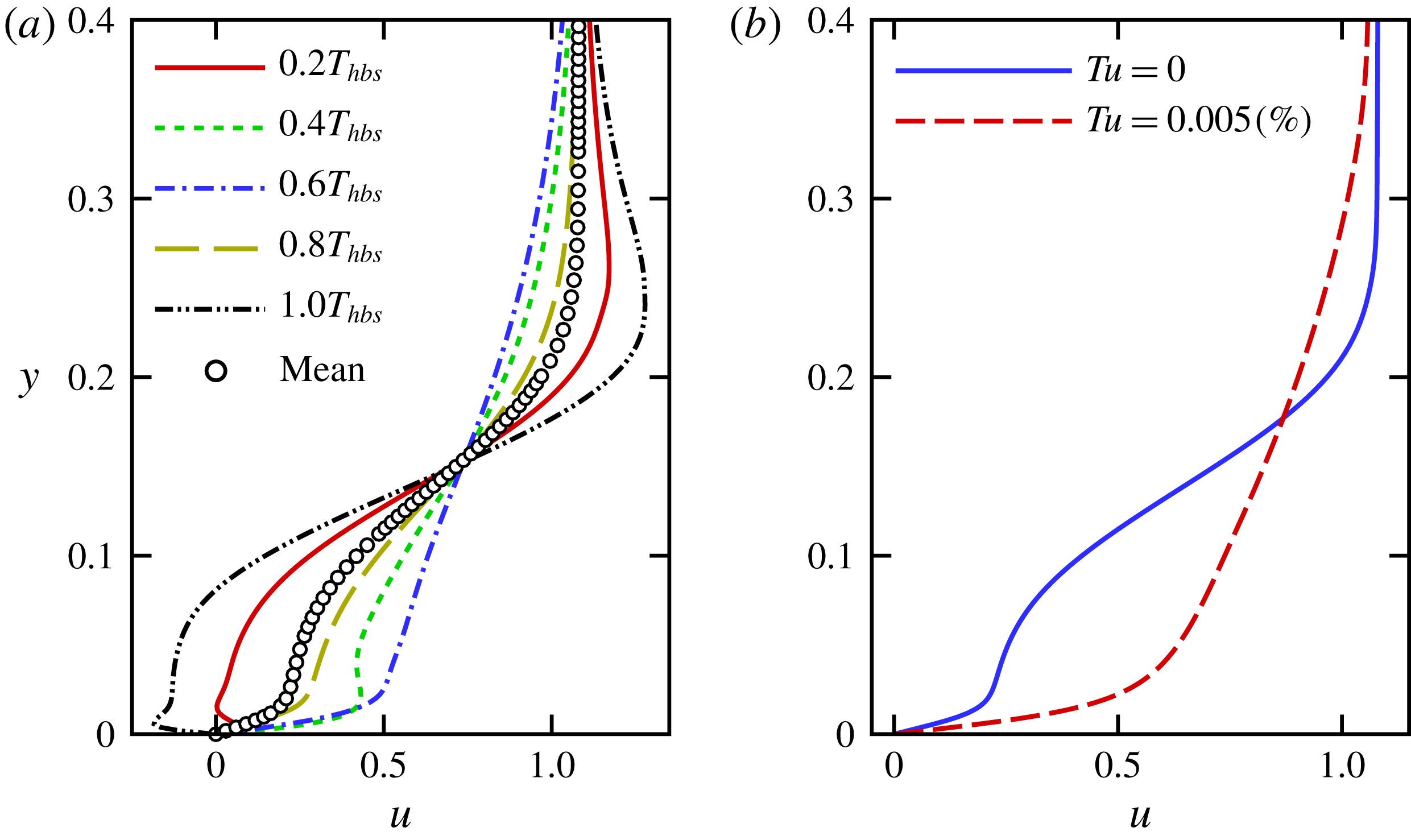
Figure 5 demonstrates that the lower skin-friction coefficient for the zero FST case, despite the train of strong spanwise vortices, is due to the intermittent reverse flow that is induced by the travelling rollers, and results in a positive but low mean u-velocity across the boundary layer as opposed to the ‘fuller’ turbulent velocity profile.

Figure 4.

(a) Comparison of skin-friction coefficients for controlled flow. (b) Time-averaged contours of the spanwise wall vorticity (top–down view) of controlled flow for zero FST (top) and $Tu=0.005\,\%$ (bottom). Dashed lines represent $\overline{\unicode[STIX]{x1D714}}_{z}=0$ .

Figure 5.

Wall-normal u-velocity profiles at $x=15$ for the controlled case with $B=0.05$ . (a) u-velocity profiles at five time instances separated by one fifth of the forcing period ( $T_{hbs}$ ) shown together with the time-averaged profile for zero FST case. (b) Comparison of the time-averaged u-velocity profile for zero FST and $Tu=0.005\,\%$ .

3.2.1 Disturbance evolution

Based on the results presented in the previous section, we conjecture that the relaminarization of the flow for the zero FST case is indeed due to the extremely low ‘noise’ level of the highly accurate DNS code, which does not occur in a practical experimental wind tunnel conditions even with very low FST. The results imply that a strong interaction between the spanwise modulations caused by FST and the primary spanwise vortices exists since the spanwise wavelength of the vortex distortions is identical to the spacing of the Klebanoff modes. By tracking the downstream development of the disturbance waves, information can be gained regarding the nature of the instability mechanisms. Toward this end, the flow data were Fourier decomposed in the spanwise direction as well as in time. The notation $(h,m)$ is used for a pair of mode numbers. Here, $h/T_{hbs}$ is the frequency where $T_{hbs}$ is the period of the actuation and $2\unicode[STIX]{x03C0}m/L_{z}$ is the spanwise wavenumber of a disturbance wave.

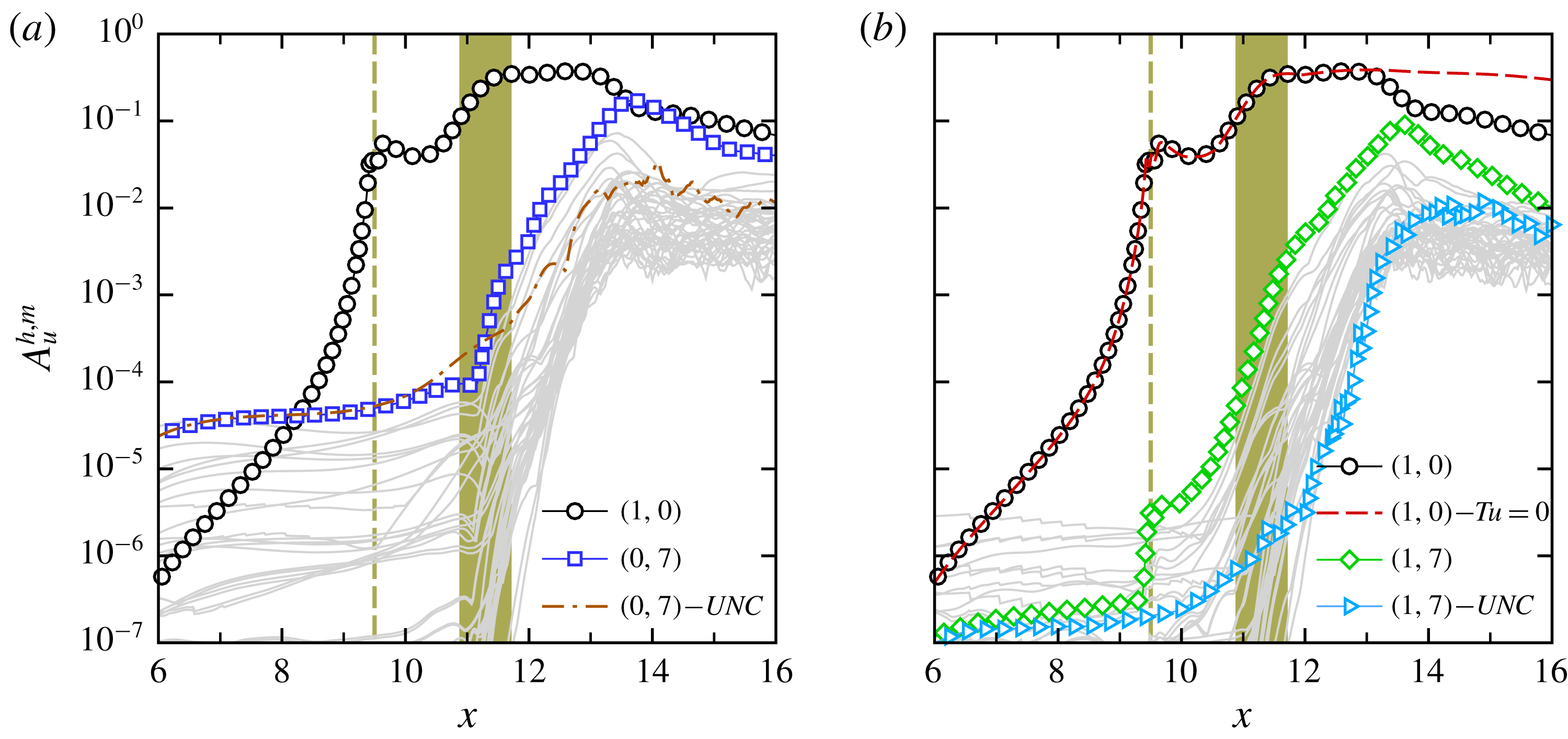
The downstream development of the maximum $u^{\prime }$ -velocity Fourier amplitude of a pair of mode numbers, $A_{u}^{h,m}$ , for the steady and unsteady disturbance waves for the controlled flow with $Tu=0.005\,\%$ is presented in figure 6; however only the modes that reach high nonlinear amplitudes are highlighted. Mode $(1,0)$ corresponds to the primary disturbance wave that is directly excited through the 2-D HBS forcing. Downstream of the forcing location, mode $(1,0)$ initially decays until $x=10.2$ , which corresponds to $Re_{cr}$ , then it experiences exponential growth and grows several orders of magnitude until nonlinear saturation sets in. In addition, it remains at much larger-amplitude levels compared to the 3-D disturbances. The 2-D mode amplitude then decays for $x>12.7$ . The beginning of the decay in the amplitude of the 2-D wave can be correlated with the onset of the spanwise modulation of the primary vortices (see figure 3 b). It should be noted that the streamwise development of mode $(1,0)$ upstream of the forcing location corresponds to the upstream influence of the excitation and is not caused by the exponential amplification of this mode.

Figure 6(a) highlights the streamwise development of the steady disturbances for various spanwise mode numbers. Although these modes have a non-zero frequency $(h\approx 0.01)$ , they are referred to as modes $(0,m)$ due to their very low frequency. Figure 6(a) clearly shows that the strongest steady 3-D disturbance wave is mode $(0,7)$ . The spanwise wavelength associated with this mode was found earlier to correspond to the spacing of the Klebanoff modes. While the K-mode grows slowly in the downstream direction prior to the separation location, it experiences very strong amplification (even higher than the primary wave) inside the separated region, until it reaches the nonlinear amplitude of the primary mode $(1,0)$ and causes the flow to break down. The streamwise evolution of the K-mode for the uncontrolled flow with $Tu=0.005\,\%$ is shown in figure 6(a) for comparison as well. The downstream growth of the K-mode for the uncontrolled case is identical to the one for the controlled case for $x<10.4$ , which is the separation location in the absence of 2-D forcing. The growth rate is enhanced downstream of the separation location, however, there is a noticeable difference in amplification rates between the controlled and uncontrolled cases, which suggests that different instability mechanisms might play a role in the presence of strong 2-D waves.

Figure 6.

Disturbance development of the Fourier amplitudes of controlled flow with $Tu=0.005\,\%$ . (a) Steady disturbance waves. (b) Unsteady modes with the forcing frequency. The vertical dashed lines correspond to the forcing location and shaded area represents the mean separated region. Also, $(0,7)-UNC$ in (a) and $(1,7)-UNC$ in (b) refer to the steady and unsteady K-modes for the uncontrolled flow with FST, respectively, and $(1,0)-Tu=0$ in (b) corresponds to the primary wave for controlled flow with zero FST.

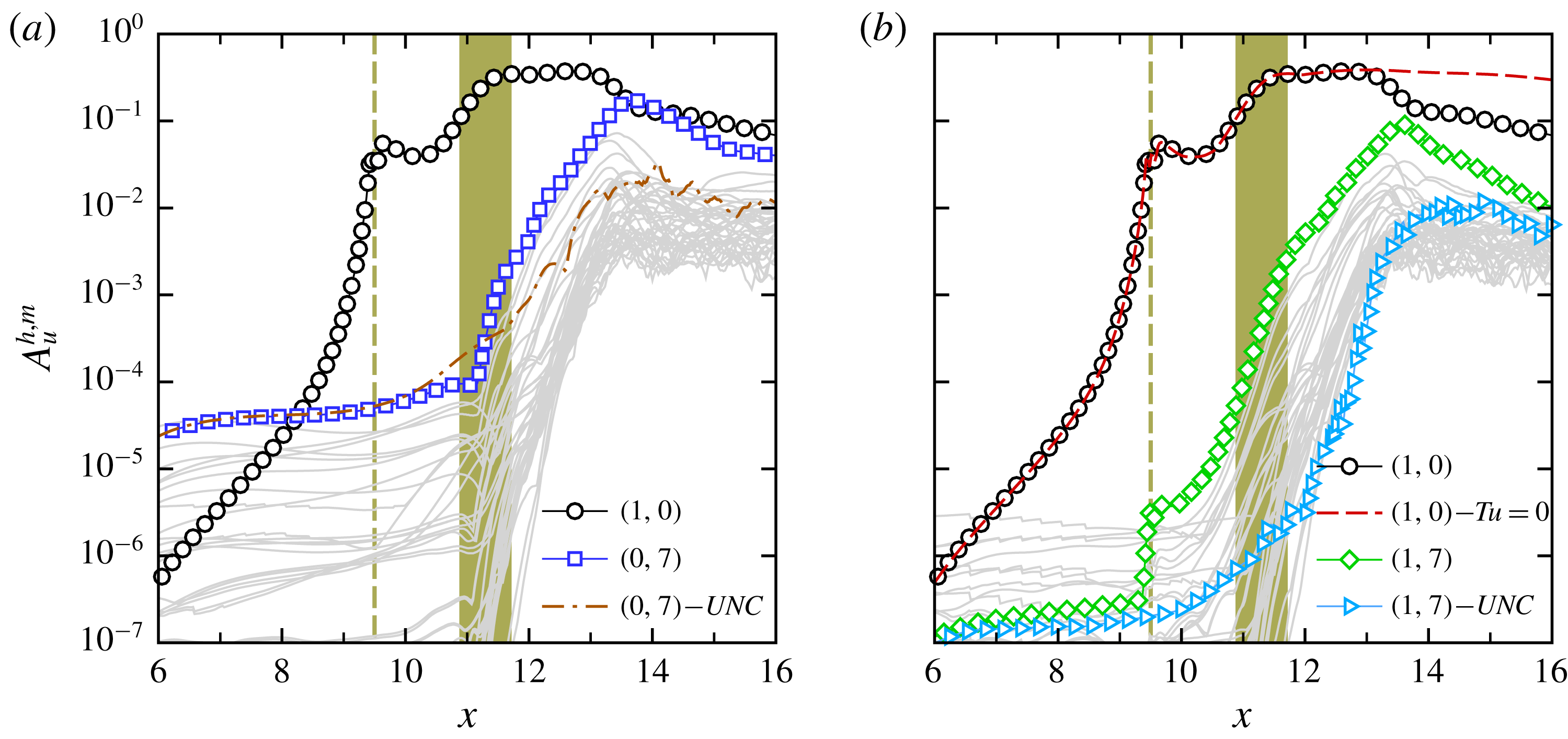
The downstream development of unsteady disturbances related to the forcing frequency, i.e. modes $(1,m)$ , is presented in figure 6(b). Whereas strong growth rates can be detected for nonlinearly generated unsteady 3-D disturbances downstream of the forcing location, the disturbance wave with the forcing frequency and the spanwise mode number of the K-mode, mode $(1,7)$ , becomes the dominant mode. This can be explained by the fact that mode $(1,7)$ is directly generated through a nonlinear wave interaction of the primary wave $(1,0)$ and the $(0,7)$ (Klebanoff) mode. Because of this nonlinear interaction, the unsteady 3-D mode $(1,7)$ assumes higher amplitude downstream of the forcing location and prevails further downstream.

The strong amplification rates detected for disturbance modes $(0,7)$ and $(1,7)$ could be an indication of a secondary instability mechanism. The secondary instability transfers kinetic energy from the large 2-D vortices to the 3-D disturbance waves. In absence of FST, this transfer is not present and hence, the 2-D primary wave remains at large amplitude levels. Therefore, the spanwise rollers remain laminar in the entire integration domain. This can be observed in figure 6(b) where the amplitude of the 2-D mode at the fundamental frequency for the controlled case with zero FST is compared with the primary 2-D wave of the case with FST.

3.2.2 Proper orthogonal decomposition

A detailed analysis of the simulation data using proper orthogonal decomposition (POD) is carried out in order to provide additional insight in the underlying flow physics and to identify the dominant structures in the transition region. POD, first proposed by Lumley (Reference Lumley1967), is a method for identifying large-scale energetic flow structures in transitional and turbulent flows. For the present results, the snapshot method, which was proposed by Sirovich (Reference Sirovich1987), is employed. In the POD method, for a given set of time ( $t$ ) and space ( $\boldsymbol{x}$ ) dependent flow data, the flow field can be represented by

(3.1)

$$\begin{eqnarray}\displaystyle & \displaystyle \boldsymbol{u}(\boldsymbol{x},t_{n})=\mathop{\sum }_{i=1}^{N}a_{i}(t_{n})\unicode[STIX]{x1D753}_{i}(\boldsymbol{x}), & \displaystyle\end{eqnarray}$$

where the $\unicode[STIX]{x1D753}_{i}$ are the POD spatial eigenfunctions and the $a_{i}$ are the POD time coefficients. The POD modes are orthogonal and optimized with respect to their energy content, i.e. the largest fraction of the total kinetic energy of the flow field is captured with the smallest number of modes. Therefore, assuming that large-scale coherent structures possess a significant amount of energy, POD can provide valuable information regarding the most relevant flow structures.

For the present modal decomposition analysis, 1500 snapshots of the velocity field $(u,v,w)^{T}$ equidistantly distributed over 50 forcing periods are used. The focus here is on identifying and extracting the dominant and coherent structures in the transitional region for controlled flow in the presence of $Tu=0.005\,\%$ from the initial linear stage all the way up to the nonlinear development of the instability waves. Therefore, the spatial extent of the snapshots was chosen from $x=6$ up to the $x=14.5$ (see figure 8).

Figure 7.

POD eigenvalue (energy) spectrum for the controlled flow with $Tu=0.005\,\%$ : (a) normalizied POD eigenvalues and (b) their cumulative energy. Spatial eigenfunctions and time signal of coloured symbols in (a) are shown in figures 8 and 9.

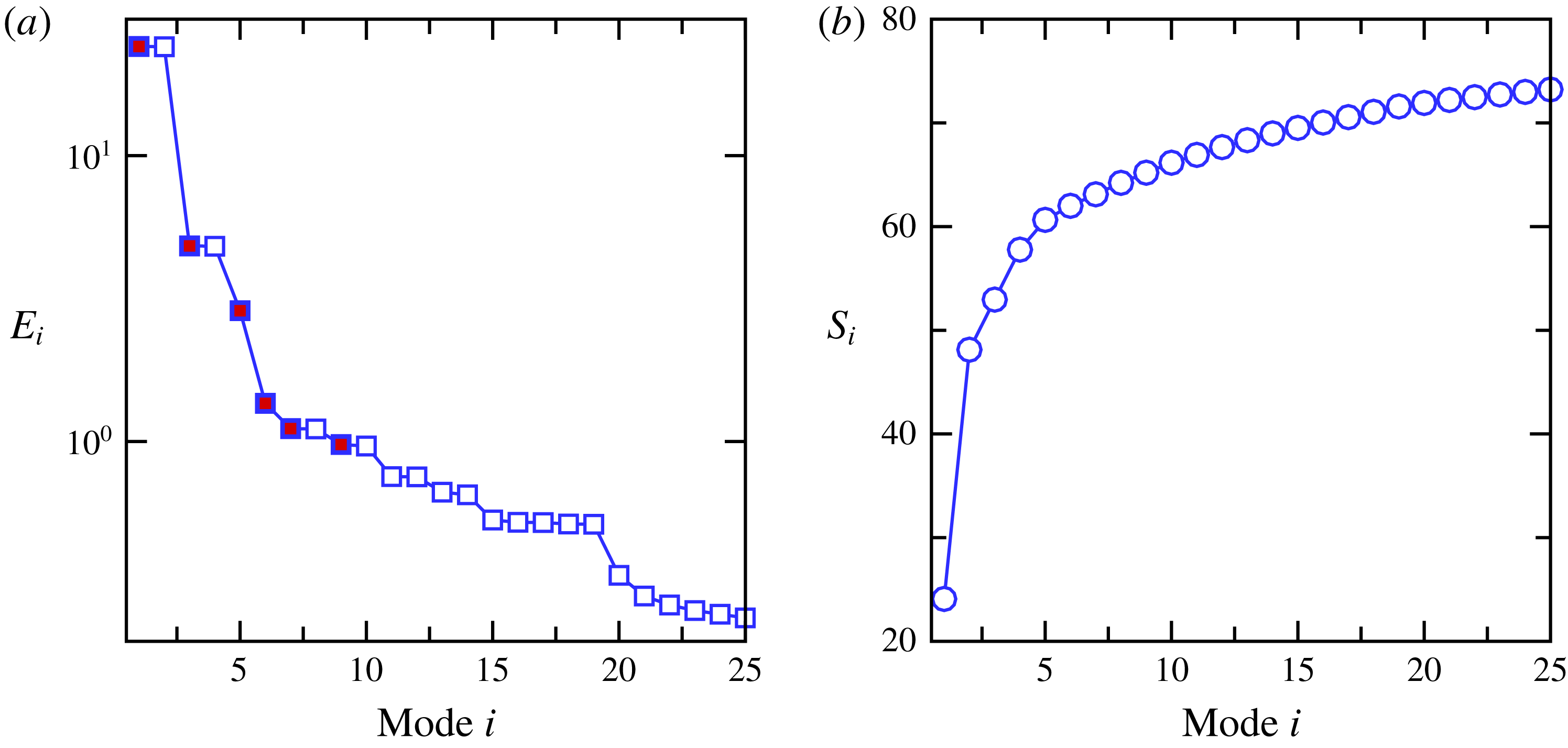
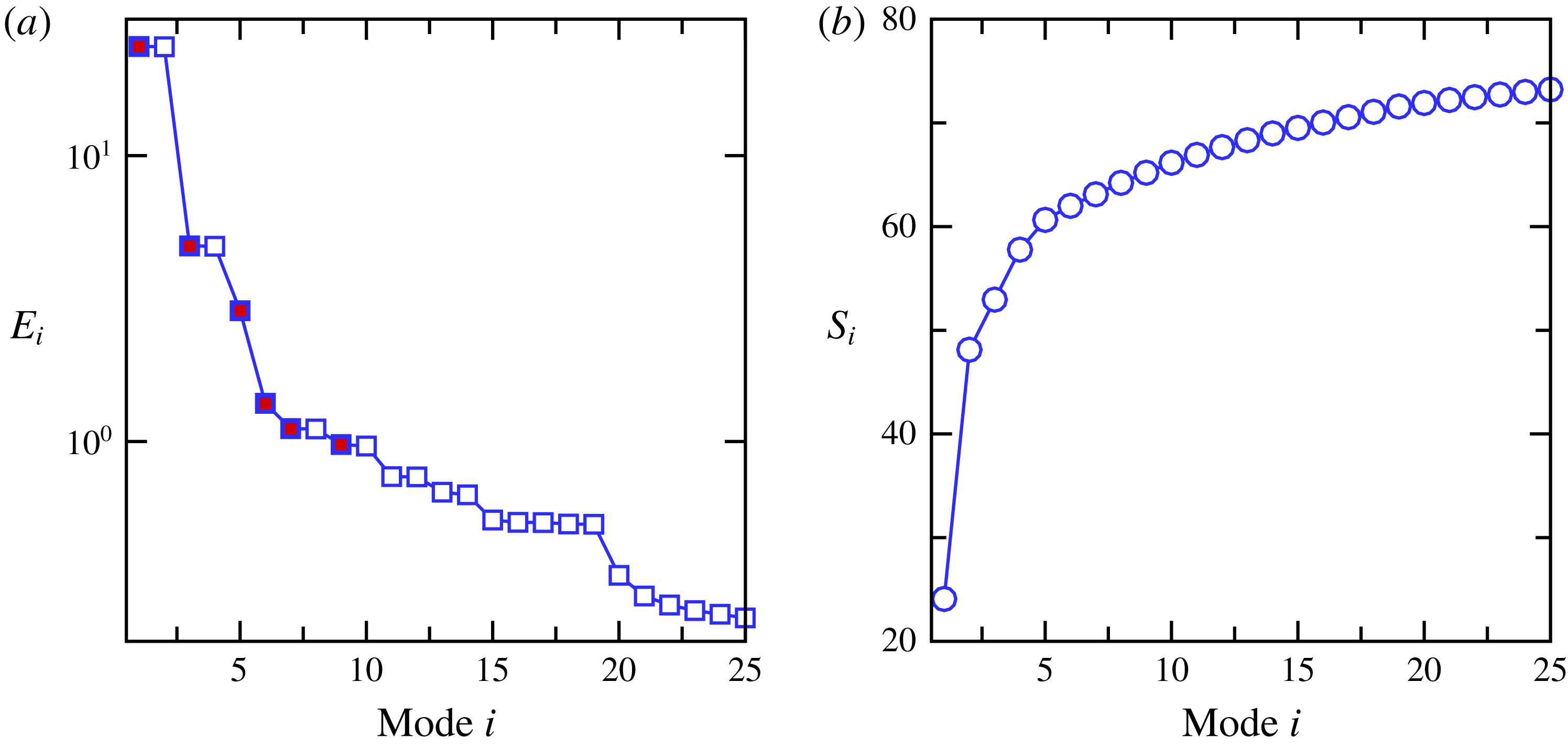
POD energy spectra are shown in figure 7 where figure 7(a) displays the contribution of each individual POD mode to the total kinetic energy, $E_{i}$ , and figure 7(b) illustrates the cumulative energy sum, $S_{i}$ , which are defined as

(3.2a,b )

$$\begin{eqnarray}\displaystyle E_{i}=\left(\unicode[STIX]{x1D706}_{i}\bigg/\mathop{\sum }_{j=1}^{N}\unicode[STIX]{x1D706}_{j}\right)\times 100,\quad S_{i}=\left(\mathop{\sum }_{k=1}^{i}\unicode[STIX]{x1D706}_{k}\bigg/\mathop{\sum }_{j=1}^{N}\unicode[STIX]{x1D706}_{j}\right)\times 100. & & \displaystyle\end{eqnarray}$$

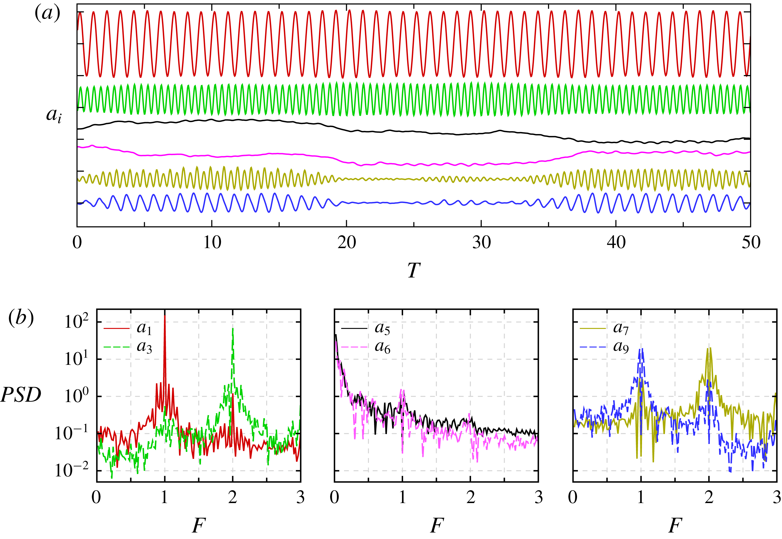
In this equation, $\unicode[STIX]{x1D706}_{i}$ is the magnitude of the eigenvalue of the POD mode, which corresponds to twice the kinetic energy content of the respective POD mode, and $N$ is the total number of POD modes. The POD eigenvalue spectra reveal that for the controlled flow, most of the energy is contained in the lower mode numbers. In particular, the most energetic modes (modes 1 and 2) contain almost $50\,\%$ of the total kinetic energy. In figure 7(a), it can be observed that the eigenvalues of the dominant POD modes, except modes 5 and 6, occur in pairs of almost equal value, whereas a large gap in magnitude exists between pairs. Each pair essentially represents the same structure, one of the eigenfunction being just shifted with respect to the other one in the streamwise direction (often referred as ‘travelling waves’, see Rempfer & Fasel Reference Rempfer and Fasel1994). Therefore, only the odd numbered modes of each pair and modes 5 and 6 are discussed here.

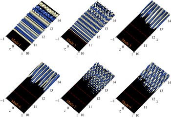
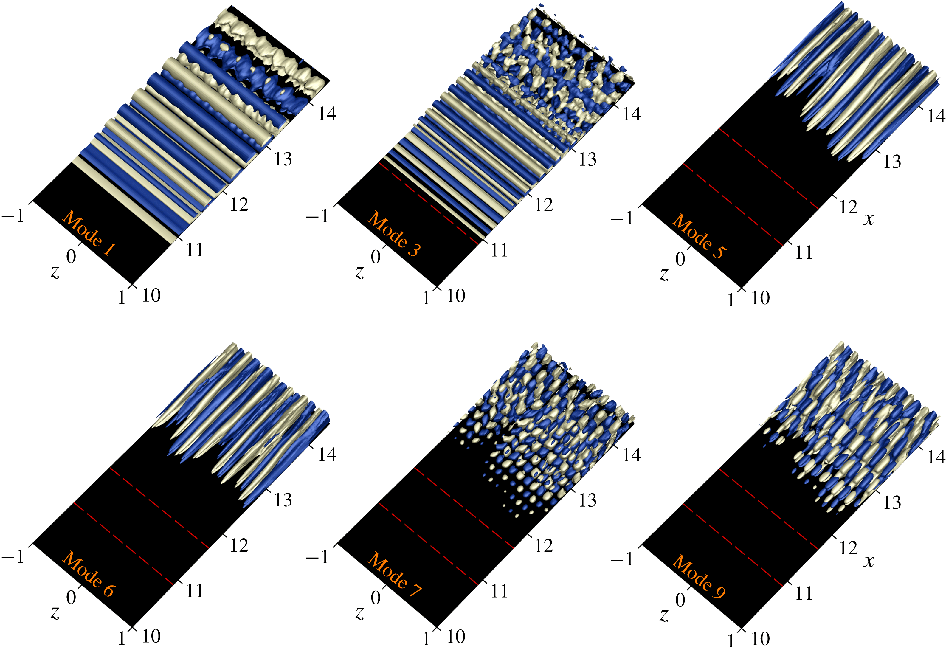
The eigenfunctions of the ‘most energetic’ POD modes are plotted in a perspective representation in figure 8, using iso-surfaces of the streamwise velocity component, $|u|=0.4$ . Figure 8 demonstrates that the most energetic structure as represented by mode 1 (and mode 2) is predominantly two-dimensional until $x<13$ from where it becomes increasingly three-dimensional further downstream. The respective time coefficient and the associated Fourier spectrum of the time coefficient (see figure 9) exhibit nearly sinusoidal behaviour with a dominant frequency matching the forcing frequency, $F=1$ . In figure 9, the time is non-dimensionalized by the forcing period, $T=t/T_{hbs}$ and similarly the frequency is non-dimensionalized by the forcing frequency, $F=f/f_{hbs}$ .

The POD eigenfunction and time coefficient for mode 3 (and mode 4) also represents (partially) the two-dimensional ‘travelling wave’ but has twice the frequency of the harmonic forcing (nonlinearly generated). The energy content of mode 3 is one fifth of that in mode 1. From the visualizations of modes 1 and 3, it can be seen that $\unicode[STIX]{x1D6FC}_{1}F_{1}\approx \unicode[STIX]{x1D6FC}_{3}F_{3}$ with $\unicode[STIX]{x1D6FC}$ being the streamwise wavelength of the structures and $F$ the dominant frequency observed for these modes. The observation of the pairs of eigenfunctions $\unicode[STIX]{x1D753}_{1}$ and $\unicode[STIX]{x1D753}_{2}$ and $\unicode[STIX]{x1D753}_{3}$ and $\unicode[STIX]{x1D753}_{4}$ , postulates that the spatially evolving coherent structures, $\unicode[STIX]{x1D6FE}(\boldsymbol{x},t)$ , can be represented by $\unicode[STIX]{x1D6FE}(\boldsymbol{x},t)=a_{i}(t)\unicode[STIX]{x1D753}_{i}(\boldsymbol{x})+a_{i+1}(t)\unicode[STIX]{x1D753}_{i+1}(\boldsymbol{x})$ , with $i$ being 1 and 3. The eigenfunction of a pair not only contains the complete information regarding the shape of the corresponding coherent structure, but also shows the evolution that the coherent structure undergoes while propagating downstream. As can be observed in figure 8, the POD modes 1 and 3 exhibit a spanwise modulation for $x>13$ which is more pronounced in mode 3.

Of particular interest in figure 8 is the observation that POD modes 5 and 6 are low-frequency streamwise oriented ‘streaky’ structures, which correspond to the Klebanoff modes caused by FST. The spanwise wavelength of these streaky structures (K-modes) is in agreement with the results found from the instantaneous visualizations (figure 3 b) and spectral analysis ( $\unicode[STIX]{x1D706}_{z,K}\approx L_{z}/7$ ). Moreover, despite their similar structures, modes 5 and 6 do not have the same energy level since they do not represent the traveling modes as was the case for modes 1 and 2 and 3 and 4.

The perspective views of modes 7 and 9 in figure 8 exhibit purely 3-D structures. In fact, they exhibit a ‘checkerboard’ pattern typically associated with oblique waves. A detailed inspection of these two modes and a comparison with the dominant modes 1, 3 and 5 reveals that modes 7 and 9 have the same spanwise wavelength as mode 5 while the streamwise wavelengths of modes 3 and 7 and modes 1 and 9 are very similar. This observation is directly linked to the mode interaction found between the primary wave and the K-mode, as identified in the spectral analysis.

Figure 8.

Dominant POD eigenfunctions for the controlled LSB with $B=0.05$ and $Tu=0.005\,\%$ . Shown are iso-surfaces of $|u|=0.4$ . Dashed red lines indicate the mean separation and reattachment locations.

Figure 9.

(a) POD time coefficients of modes 1 (red), 3 (green), 5 (black), 6 (purple), 7 (dark yellow) and 9 (blue). (b) Associated frequency spectra. Controlled LSB with $B=0.05$ in the presence of FST with $Tu=0.005\,\%$ .

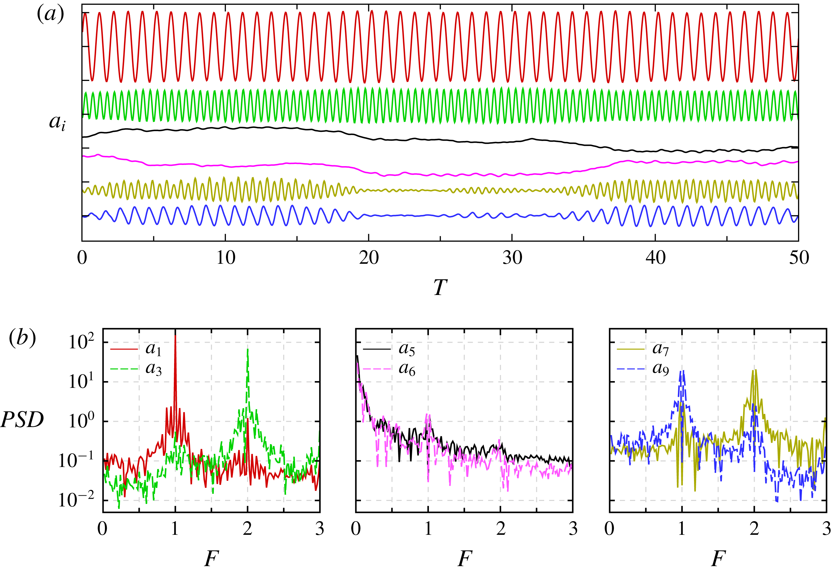
The time signals for modes 7 and 9 (figure 9 a, right plot) are reminiscent of ‘modulated wave trains’ and are qualitatively similar to those observed by Schubauer & Skramstad (Reference Schubauer and Skramstad1948) in their classical ‘natural’ transition experiments of a flat-plate boundary layer. The corresponding frequency spectrum (figure 9 b, right plot) exhibits a dominant frequency peak close to $2f_{hbs}$ and $f_{hbs}$ , respectively. It is important to note that for POD modes 7 and 9, their dominant frequencies do not occur at $2f_{hbs}$ and $f_{hbs}$ but instead at $2f_{hbs}\pm f_{K}$ and $f_{hbs}\pm f_{K}$ , respectively, (as you could see from a close-up view of figure 9 b, right plot) where $f_{K}$ is the frequency associated with the ‘streaky’ structures as observed in POD mode 5 (figure 9 b, middle plot).

Linking the dominant POD modes to the spectral analysis from previous section, confirms that POD modes 1 and 2 correspond to the primary wave, that POD modes 5 and 6 represent mode $(0,7)$ which was identified in the spectral analysis as the instability mode causing the laminar–turbulent transition, and that POD modes 9 and 10 have close similarity to mode $(1,7)$ . Moreover, POD modes 3 and 4 and 7 and 8 are higher harmonics that are nonlinearly generated.

3.2.3 Secondary instability investigations

Results presented in the previous sections revealed that the spanwise wavelength of the observed modulation of ‘rollers’ in the transition region is governed by the spanwise spacing of the Klebanoff modes inside the boundary layer. This scenario suggests that a secondary instability analysis of the two-dimensional time-periodic disturbance wave with respect to steady (or low-frequency) spanwise sinusoidal disturbances may be helpful for identifying the relevant physical mechanism that cause the modulation as observed in figure 3(b). Secondary instability investigations can also gain insight into the receptivity of the secondary instability regime of a forced (‘controlled’) LSB with respect to the low-frequency 3-D disturbances.

The goal of this secondary stability analysis is to obtain a range of unstable wavenumbers for comparison with the dominant spanwise wavelength as identified in the previous sections. The fact that the secondary instability mechanism is a linear mechanism, it is therefore, accessible using the linearized Navier–Stokes equations (LNSE) and employing a Floquet-type analysis. Towards this end, we developed an approach that directly solves the LNSE where time-dependent solutions from DNS serve as a base flow (or basic flow) without using any additional assumptions as required by the standard secondary instability analysis (i.e. assuming the mean flow is locally parallel, the amplitude of primary wave is independent of $x$ , and requiring a ‘shape assumption’ that the primary wave does not change its shape as it saturates; see Herbert Reference Herbert1988). Thus, all ‘non-parallel’ effects with respect to the base flow and the primary wave are included in the LNSE approach, which is important as separated flows are considered here.

For the secondary instability analysis employed here based on LNSE, the total flow field is decomposed into the unsteady base flow and disturbance flow

(3.3a )

$$\begin{eqnarray}\displaystyle & \displaystyle \boldsymbol{u}(x,y,z,t)=\boldsymbol{u}_{B}(x,y,t)+\boldsymbol{u}^{\prime }(x,y,z,t), & \displaystyle\end{eqnarray}$$

(3.3b )

$$\begin{eqnarray}\displaystyle & \displaystyle \unicode[STIX]{x1D74E}(x,y,z,t)=\unicode[STIX]{x1D74E}_{B}(x,y,t)+\unicode[STIX]{x1D74E}^{\prime }(x,y,z,t). & \displaystyle\end{eqnarray}$$

Substituting these decompositions into the Navier–Stokes equations (2.1), yields the governing equations for the total flow field, which after linearization (by neglecting products of the disturbance quantities), is a linear superposition of the base flow and the disturbance flow. Thus, the governing equations for the base flow can be subtracted from the equations for the total flow in order to obtain the LNSE with the unsteady base flow,

(3.4)

$$\begin{eqnarray}\displaystyle & \displaystyle {\displaystyle \frac{\unicode[STIX]{x2202}\unicode[STIX]{x1D74E}^{\prime }}{\unicode[STIX]{x2202}t}}=\unicode[STIX]{x1D735}\times (\boldsymbol{u}^{\prime }\times \unicode[STIX]{x1D74E}_{B}+\boldsymbol{u}_{B}\times \unicode[STIX]{x1D74E}^{\prime })+{\displaystyle \frac{1}{Re}}\unicode[STIX]{x1D6FB}^{2}\unicode[STIX]{x1D74E}^{\prime }-\unicode[STIX]{x1D735}\times \boldsymbol{{\mathcal{F}}}. & \displaystyle\end{eqnarray}$$

The disturbance velocity field can be obtained from $\unicode[STIX]{x1D6FB}^{2}\boldsymbol{u}^{\prime }=\unicode[STIX]{x1D735}\times \unicode[STIX]{x1D74E}^{\prime }$ . In the above equation, $\boldsymbol{{\mathcal{F}}}$ is a volume force. For numerically solving the LNSE, the same time integration and spatial discretization schemes are employed as for the nonlinear equations used in the DNS. To analyse the stability with respect to 3-D (oblique) disturbance waves when the base flow is two-dimensional, a spectral discretization in the z-direction is implemented into the linearized solver. Since the base flow is homogeneous in the spanwise direction, the perturbation can be further decomposed, such that

(3.5a )

$$\begin{eqnarray}\displaystyle & \displaystyle \unicode[STIX]{x1D753}^{\prime }(x,y,z,t)=\mathop{\sum }_{m=0}^{M}\widehat{\unicode[STIX]{x1D753}}_{m}(x,y,t)~\cos (\unicode[STIX]{x1D6FD}_{m}z), & \displaystyle\end{eqnarray}$$

(3.5b )

$$\begin{eqnarray}\displaystyle & \displaystyle \unicode[STIX]{x1D74D}^{\prime }(x,y,z,t)=\mathop{\sum }_{m=0}^{M}\widehat{\unicode[STIX]{x1D74D}}_{m}(x,y,t)~\sin (\unicode[STIX]{x1D6FD}_{m}z), & \displaystyle\end{eqnarray}$$

where

$\unicode[STIX]{x1D753}=[u,v,\unicode[STIX]{x1D714}_{z}]^{\text{T}}$ ,

$\unicode[STIX]{x1D74D}=[w,\unicode[STIX]{x1D714}_{x},\unicode[STIX]{x1D714}_{y}]^{\text{T}}$ and

$\unicode[STIX]{x1D6FD}_{m}$ is the spanwise wavenumber. Since the linearized equations are solved, Fourier modes with different

$\unicode[STIX]{x1D6FD}_{m}$ are decoupled and can be analysed separately. The time-dependent two-dimensional base flow,

$\boldsymbol{u}_{B}=[u_{B},v_{B},0]^{\text{T}}$ and

$\unicode[STIX]{x1D74E}_{B}=[0,0,\unicode[STIX]{x1D714}_{z,B}]^{\text{T}}$ , is a superposition of a steady part (time averaged) and

$N$ downstream travelling waves,

(3.6)

$$\begin{eqnarray}\displaystyle & \displaystyle \unicode[STIX]{x1D6F9}_{B}(x,y,t)=\unicode[STIX]{x1D6F9}_{0}(x,y)+\mathop{\sum }_{n=1}^{N}\unicode[STIX]{x1D6F9}_{A}^{(n)}(x,y)~\cos [2\unicode[STIX]{x03C0}nf_{hbs}t+\unicode[STIX]{x1D6F9}_{ph}^{(n)}(x,y)], & \displaystyle\end{eqnarray}$$

where $\unicode[STIX]{x1D6F9}=[u,v,\unicode[STIX]{x1D714}_{z}]^{\text{T}}$ and $\unicode[STIX]{x1D6F9}_{0}$ corresponds to the two-dimensional steady flow that is identical to the temporal mean of the total flow field (velocity and vorticity). The unsteady part consists of a fundamental wave ( $f_{hbs}$ ) and its first ( $N-1$ ) higher harmonics propagating in the downstream direction. Amplitudes ( $\unicode[STIX]{x1D6F9}_{A}$ ) and phase distributions ( $\unicode[STIX]{x1D6F9}_{ph}$ ) of these waves are obtained from a Fourier analysis of the total flow provided by DNS.

To generate streamwise vortices outside the boundary layer in the LNSE solver for the SIA, a (unsteady) volume force $\boldsymbol{{\mathcal{F}}}(\boldsymbol{x},t)=[f_{u},f_{v},f_{w}]^{\text{T}}$ is added to the LNSE. Its components are $f_{u}=0$ , $f_{v}=0$ and

(3.7)

$$\begin{eqnarray}\displaystyle & \displaystyle f_{w}(\boldsymbol{x},t)=\mathop{\sum }_{m=0}^{M}\widehat{f}_{w,m}\exp \left[-\left({\displaystyle \frac{x-xc_{m}}{a_{m}}}\right)^{2}-\left({\displaystyle \frac{y-yc_{m}}{b_{m}}}\right)^{2}\right]\sin (\unicode[STIX]{x1D6FD}_{m}z)~\cos (\unicode[STIX]{x1D6FA}_{m}t). & \displaystyle\end{eqnarray}$$

In (3.7), $xc_{m}$ , $yc_{m}$ , $a_{m}$ and $b_{m}$ define the shape of the forcing of each spanwise Fourier mode, $\unicode[STIX]{x1D6FD}_{m}$ , $\widehat{f}_{w,m}$ is the amplitude and $\unicode[STIX]{x1D6FA}_{m}$ is the angular frequency. For the specific values used in the present investigation see table 1. In the calculations, the curl $\unicode[STIX]{x1D735}\times {\mathcal{F}}$ is used as a source term on the right-hand side of the linearized vorticity transport equation. Regarding the computational parameters given in table 1, it is worth noting that the frequency is chosen according to the frequency associated with the K-mode obtained from the Fourier analysis and the wall-normal location of the volume force is approximately 2.5 of the local boundary-layer thickness.

It should be noted that no perturbations from the FST model (continuous modes) are used in the secondary instability investigations. Instead, in the linearized calculations the source term, equation (3.7), is employed to generate the streamwise vortices close to the inflow boundary and outside the boundary layer. This numerical model was successfully implemented by Fasel (Reference Fasel2002) to generate low-frequency vortices outside the boundary layer in order to excite Klebanoff modes inside the boundary layer. Making use of the observation in figure 3(a) that the controlled flow with zero FST is predominantly two-dimensional, a 2-D simulation with $B=0.05$ is carried out to obtain the unsteady base flow required for SIA. The flow data are sampled with a time interval of $\unicode[STIX]{x0394}t=T_{hbs}/30$ for 12 forcing periods. Then, the time-dependent data were Fourier transformed in time to provide the amplitude and phase distributions.

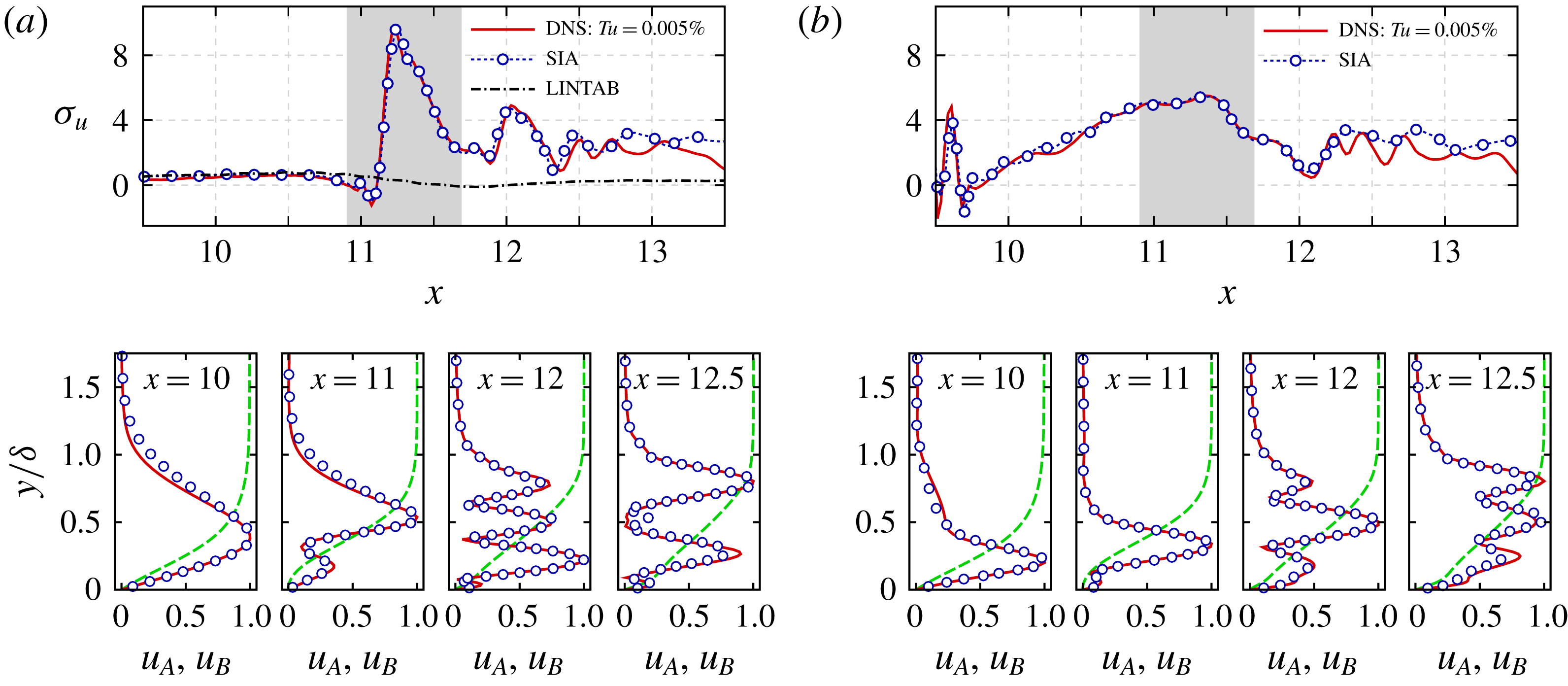
In figure 10, the spatial growth rates and $u^{\prime }$ -velocity Fourier amplitude profile ( $u_{A}$ ) of the three-dimensional mode with $\unicode[STIX]{x1D6FD}_{m}\approx 22$ , which corresponds to the lateral wavelength of the K-mode ( $\unicode[STIX]{x1D706}_{z}\approx 0.286$ ), are plotted as obtained from the SIA and are compared with the DNS results of a controlled LSB with $Tu=0.005\,\%$ . The local growth rate is computed based on the wall-normal maxima of the $u_{A}$ according to $\unicode[STIX]{x1D70E}_{u}(x)=\unicode[STIX]{x2202}\log (u_{A,max})/\unicode[STIX]{x2202}x$ . In figure 10, the Fourier amplitudes are scaled by their respective maximum amplitudes and $u_{B}$ is the corresponding time-averaged $u$ -velocity profile normalized by its boundary-layer edge value. The growth rates of the K-modes obtained from the SIA compare very well with those from the DNS for mode $(0,7)$ and mode $(1,7)$ as shown in figure 10(a,b), respectively. Comparison of wall-normal distributions of the disturbance amplitude in figure 10 (bottom plots) confirms the proper implementation and accuracy of the unsteady base flow method for the SIA. It is important to note that mode $(1,7)$ is not forced in the LNSE calculations, but generated due to the unsteady component of the base flow.

Table 1.

Computational parameters used to define the volume force in (3.7).

Figure 10.

Comparison of local spatial growth rates (top) and wall-normal distributions of the $u^{\prime }$ -velocity Fourier amplitudes at several x-locations (bottom) obtained from SIA and DNS with $Tu=0.005\,\%$ : (a) mode $(0,7)$ ; (b) mode $(1,7)$ . Disturbance amplitudes are scaled by their respective maximum. Dashed lines in the bottom plots represent the corresponding time-averaged $u$ -velocity profile normalized by the edge velocity. LINTAB in (a) refers to linear calculation for mode (0,7) based on the time-averaged base flow. Shaded area indicates the mean separated region. Wall-normal coordinates are normalized by the local boundary-layer thickness.

Figure 10(a) also provides the growth rate of the K-mode as computed from the linearized Navier–Stokes equations when only the time-averaged part of the base flow is considered (dot-dash curve), hereinafter referred to as ‘LINTAB’. The terminology ‘LINTAB’ is introduced to distinguish this approach (stability calculation using LNSE based on the time-averaged base flow) from the SIA (secondary stability calculation using LNSE based on the time-dependent base flow). As displayed in figure 10(a), the growth rates, $\unicode[STIX]{x1D70E}_{u}$ , from the LINTAB are identical to those obtained from SIA and DNS calculations up to the separation location and remain almost unchanged thereafter while the SIA and DNS results show much larger amplification rates. Therefore, this analysis confirms that the growth rate identified for mode $(0,7)$ is indeed caused by the unsteady component (due to the 2-D forcing) of the base flow while the instability of the mean flow only has negligible effect.

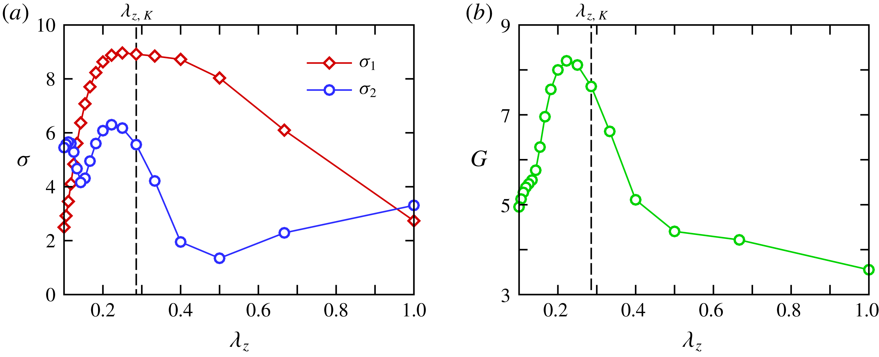
Next, results from calculations for disturbances with a wide range of spanwise wavelengths are presented in order to identify the band of unstable wavelengths. The spatial growth rates of the steady modes as computed based on the spectral disturbance kinetic energy (SDKE), are plotted in figure 11(a) as a function of the spanwise disturbance wavelength. The SDKE is computed from the wall-normal integral of the Fourier amplitude of the velocity components according to

(3.8)

$$\begin{eqnarray}\displaystyle q(x)={\displaystyle \frac{1}{\unicode[STIX]{x1D6FF}(x)}}\int _{0}^{\unicode[STIX]{x1D6FF}(x)}{\displaystyle \frac{1}{2}}[u_{A}^{2}(x,y)+v_{A}^{2}(x,y)+w_{A}^{2}(x,y)]\,\text{d}y, & & \displaystyle\end{eqnarray}$$

where $\unicode[STIX]{x1D6FF}(x)$ is the local boundary-layer thickness. Furthermore, the energy growth ratio, $G=\log _{10}[q(x=13.5)/q(x=10)]$ , is introduced to evaluate the disturbance amplification from the results of the SIA and is shown in figure 11(b).

In figures 6 and 10 it was seen that the growth rates of the 3-D disturbances vary upstream of the mean reattachment location and even until $x=12.5$ , while a nearly constant exponential growth rate is observed further downstream. Therefore, two growth rates, $\unicode[STIX]{x1D70E}_{1}$ and $\unicode[STIX]{x1D70E}_{2}$ , are observed in figure 11(a) where $\unicode[STIX]{x1D70E}_{1}$ is the averaged growth rate for $11\leqslant x\leqslant 12.5$ and $\unicode[STIX]{x1D70E}_{2}$ is an exponentially fitted growth rate for $x>12.5$ . What is significant in figure 11(a) is that the range of unstable 3-D modes is very broad. From the spanwise variation of $\unicode[STIX]{x1D70E}_{1}$ , it appears that the most unstable 3-D disturbances have a wavelength in the range of $0.2\leqslant \unicode[STIX]{x1D706}_{z}\leqslant 0.4$ . In that range, the dependency of the growth rate on the wavelength is less pronounced and $\unicode[STIX]{x1D70E}_{1}$ stays almost constant. On the other hand, judging from the energy growth ratio $G$ and $\unicode[STIX]{x1D70E}_{2}$ , the most unstable spanwise wavelength is $\unicode[STIX]{x1D706}_{z}\approx 0.22$ . Of particular interest, however, is the observation that the wavelength associated with the spanwise spacing of the K-mode, i.e. $\unicode[STIX]{x1D706}_{z,K}\approx 0.29$ , falls into the range of, and is in fact very close to, the most unstable 3-D disturbances.

Figure 11.

Results from the secondary instability analysis of the controlled flow with $B=0.05$ for steady disturbances. (a) Growth rate ( $\unicode[STIX]{x1D70E}$ ) of disturbances as a function of spanwise wavelength where $\unicode[STIX]{x1D70E}_{1}$ corresponds to the averaged $\unicode[STIX]{x1D70E}$ over $11\leqslant x\leqslant 12.5$ , and $\unicode[STIX]{x1D70E}_{2}$ represents the exponentially fitted $\unicode[STIX]{x1D70E}$ for $x>12.5$ . (b) Variation of energy growth ratio versus spanwise wavelength. The spanwise wavelength of the K-mode, $\unicode[STIX]{x1D706}_{z,K}$ , is marked by vertical dashed lines.

It is important to note, however, that the SDKE of the K-mode is order(s) of magnitude larger than that of the other low-frequency 3-D disturbances according to the spectral analysis results obtained from DNS of controlled flow with $Tu=0.005\,\%$ . In fact, the SDKE of disturbances with $\unicode[STIX]{x1D706}_{z}\approx 0.22$ , the dominant mode from SIA, is 4–5 orders of magnitude lower than the one with $\unicode[STIX]{x1D706}_{z}\approx 0.29$ (K-mode). Therefore, considering the large initial amplitude, the high growth rate and large energy growth ratio of disturbance waves with $\unicode[STIX]{x1D706}_{z}\approx 0.29$ , it can be concluded that such disturbances will dominate the transition process.

3.3 Effect of forcing amplitude

The results presented thus far indicate that the laminar–turbulent transition for the forced LSB in the presence of FST is directly linked to the interaction of low-amplitude K-modes with the high-amplitude 2-D mode associated with the flow control. Thus, the question arises if and how varying the 2-D forcing amplitude ( $B$ ) affects this interaction. In order to answer this question, secondary instability analyses using the LNSE approach (as described in the previous section) are carried out for $0.008\leqslant B\leqslant 0.07$ . For brevity only the evolution of low frequency 3-D disturbances with a spanwise wavelength equal to the one of the K-mode is examined.

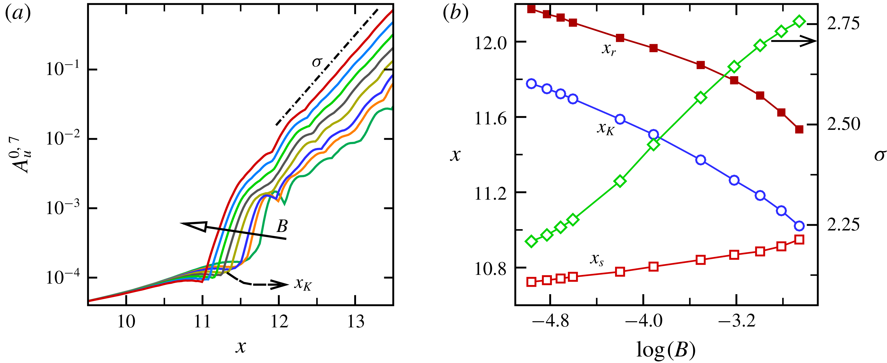
Figure 12(a) shows the streamwise amplitude development of mode $(0,7)$ for different forcing amplitudes. Figure 12(b) provides the mean separation/reattachment locations ( $x_{s}$ , $x_{r}$ ), as well as the onset locations of the growth of the K-modes ( $x_{K}$ ) as a function of the forcing amplitude. Also, included in figure 12(b) is the variation of the exponential amplification rate measured downstream of $x_{r}$ as a function of $B$ . Whereas the downstream development of the K-modes suggests that the underlying instability characteristic is similar for different forcing amplitudes, figure 12 also points to some interesting aspects when $B$ decreases: (i) the growth of the disturbance waves is delayed and (ii) the exponential amplification rate of the 3-D modes is reduced. It can therefore be conjectured that the combined effect of these two events is that, for reduced forcing amplitudes, transition is delayed.

To further investigate the effect of forcing amplitude and verify the results predicted from SIA, DNS are carried out for two additional forcing amplitudes $B=0.01$ and $B=0.025$ for the same FST as before ( $Tu=0.005\,\%$ ). The forcing slot for the DNS was located at the end of favourable-pressure-gradient region where the local boundary-layer edge velocity is $u_{e}=1.37U_{\infty }$ . Based on this local condition, the effective forcing amplitude is therefore, approximately $3.65\,\%$ , $1.82\,\%$ and $0.73\,\%$ of the free-stream velocity for $B=0.05$ , $0.025$ and $0.01$ , respectively. As can be observed in figure 6 for $B=0.05$ , for example, the disturbances introduced at $x=9.5$ initially decay until $x=10.2$ and start to grow thereafter. Hence, a smaller forcing amplitude can be introduced downstream of $Re_{cr}$ while still having the same effect as for the ones observed with $B=0.05$ .

Figure 12.

(a) Streamwise development of the K-mode obtained from SIA for controlled flow with different forcing amplitudes $B$ . (b) Mean separation/reattachment locations ( $x_{s}$ , $x_{r}$ ) as well as onset locations of K-mode growth ( $x_{K}$ ) as a function of $\log (B)$ . Right vertical axis in (b) is the exponential growth rate of the K-mode measured downstream of $x_{r}$ .

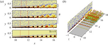
Instantaneous contours of spanwise vorticity from DNS as shown in figure 13(a), corroborate the SIA results, namely that transition is delayed for smaller forcing amplitudes. In fact, four 2-D ‘laminar’ spanwise ‘rollers’ are visible for $B=0.01$ compared to only two ‘rollers’ for $B=0.05$ . The mean separation and reattachment locations are indicated in figure 13(a) by vertical dashed lines for each case. Thus the DNS results confirm the predictions made from figure 12(b), i.e. a reduction of the bubble size (due to delayed separation and earlier reattachment) with increasing forcing amplitudes. Contours of spanwise vorticity for $B=0.01$ in the absence of FST are also shown in figure 13(a) for comparison purposes, which demonstrates, similarly to the case with $B=0.05$ presented in figure 3, that the strength of the 2-D rollers alone could determine the extent of the mean separated region and that this extent is independent of the FST. In fact, for every 2-D vortex in zero FST simulation, there are modulated but still laminar ‘rollers’ in the DNS with $Tu=0.005\,\%$ until approximately $x=15$ where the spanwise structures become strongly distorted (‘shredded’) as can be observed in figure 13(b) for $B=0.01$ .

The perspective view of the dominant flow structures (identified using iso-surfaces of $\unicode[STIX]{x1D706}_{2}=-40$ ) in figure 13(b), provides an overview of the transition process for this case. The dominant flow structures look similar to those from the DNS with $B=0.05$ as presented in figure 3(b) where the modulated structures with the spanwise wavelength of the K-mode lead to the laminar-to-turbulent transition. 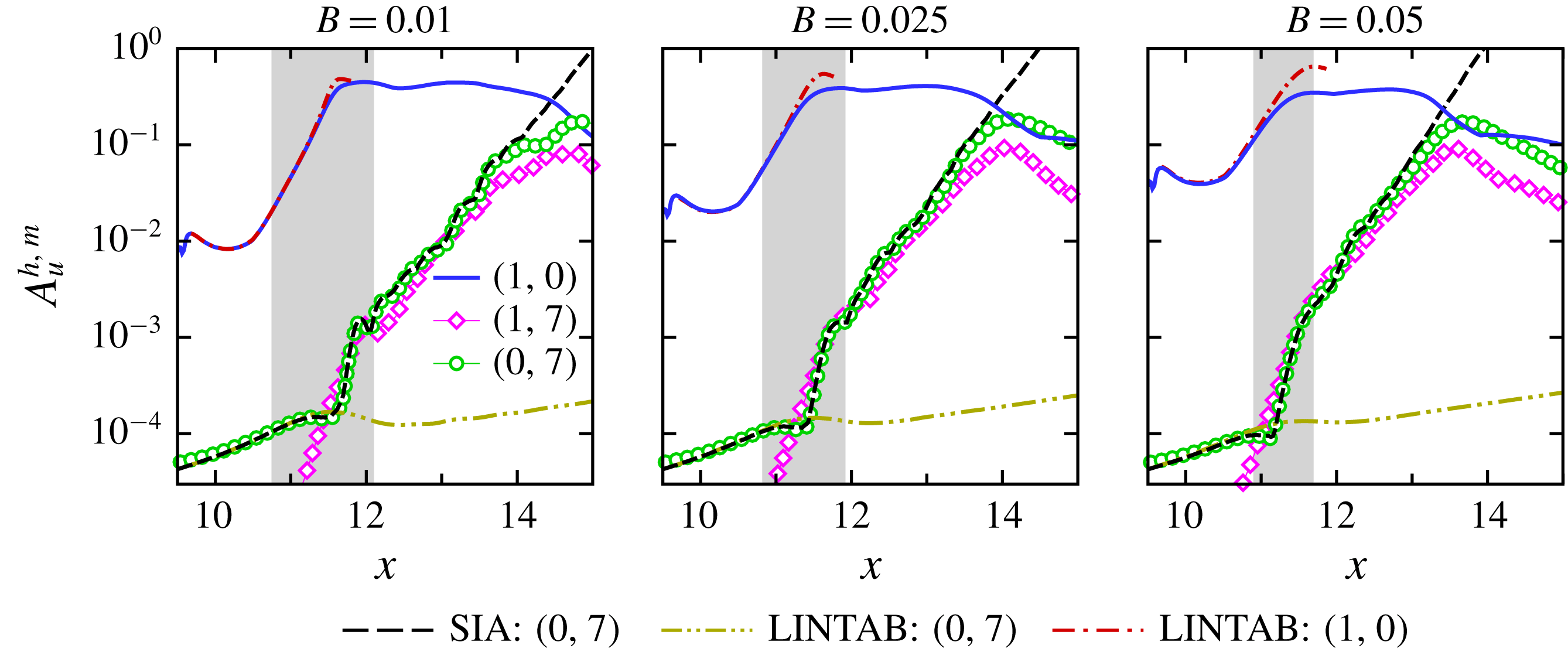However, for the case with $B=0.01$ the modulation takes place further downstream, and as a consequence of this, transition is delayed as compared to the case with $B=0.05$ (see figure 3 b). This conclusion is further supported by the streamwise development of the Fourier amplitudes as presented in figure 14. Shown are comparisons of the downstream development of the maximum $u^{\prime }$ -velocity Fourier amplitude ( $A_{u}^{h,m}$ ) of modes $(1,0)$ and $(0,7)$ for the controlled flow with $Tu=0.005\,\%$ for three forcing amplitudes. In addition to results from DNS, figure 14 includes the results from SIA for mode $(0,7)$ as well as the streamwise development of the same mode computed with the LINTAB approach (LNSE based on the time-averaged base flow only).

Figure 13.

(a) Instantaneous contours of the spanwise-averaged spanwise vorticity and contour lines (blue dashed) of $\ln (|\unicode[STIX]{x1D714}_{z}|)$ for different forcing amplitudes with $Tu=0.005\,\%$ . From top to bottom: $B=0.05$ , $B=0.025$ and $B=0.01$ . The bottom plot was obtained from a zero FST simulation with $B=0.01$ . (b) Perspective view of instantaneous flow visualization for the case with $B=0.01$ . Plotted are iso-surfaces of $\unicode[STIX]{x1D706}_{2}=-40$ coloured by $u$ -velocity.

Figure 14.

Streamwise development of primary wave, $(1,0)$ , and K-mode, $(0,7)$ , for different forcing amplitudes. Shown also is the streamwise amplitude development for modes $(1,0)$ and $(0,7)$ computed with LINTAB (time-averaged base flow) and SIA (time-dependent base flow) for mode $(0,7)$ . The mean separated region is identified by shaded area.

The evolution of mode $(1,0)$ illustrates the dependency of the stability characteristics of the mean flow on the amplitude of the forcing, namely, a stabilization of the convective instability of the separated boundary layer with increasing forcing amplitude. Similar observations were reported by Marxen & Rist (Reference Marxen and Rist2010) and Marxen & Henningson (Reference Marxen and Henningson2011). Once the 2-D mode saturates (at a nonlinear, finite amplitude), it remains at much larger-amplitude levels compared to the 3-D disturbances. The break down occurs when the amplitude of the K-mode reaches the level of the primary mode. In agreement with the results in figure 12, the strong amplification of the K-mode moves downstream as the forcing amplitude decreases. Consequently, the beginning of the amplitude decay of mode $(1,0)$ is delayed. Thus, the net consequence is a delay of laminar–turbulent transition.

In agreement with the previous findings (in figure 10, top plot) for $B=0.05$ , figure 14 indicates that the convective instability characteristic of the mean flow is very weak with respect to low-frequency 3-D disturbance waves. Moreover, the significant increase in the amplification rate of mode $(0,7)$ as observed from the DNS and SIA for smaller forcing amplitudes, is caused by the unsteady part of the base flow. Also included in figure 14 is the evolution of the primary wave computed with the LINTAB approach. The base flows for the LINTAB investigations are the time-averaged flow fields obtained from DNS for various forcing amplitudes. Excellent agreement between the LINTAB and DNS results in the region of exponential growth for $B=0.01$ provides strong support that the evolution of the 2-D mode before saturation is indeed an entirely linear mechanism and that nonlinear effects are negligible. Although the overall agreement between the DNS and LINTAB for mode $(1,0)$ for $B=0.05$ is good, a closer inspection of figure 14 (right plot) reveals that the growth of the 2-D mode obtained from DNS deviates slightly from the one computed using the LINTAB downstream of the separation location. This could be an indication of nonlinearity caused by a large-amplitude forcing.

3.4 Effect of free-stream turbulence level

The results presented so far were for a fixed FST intensity of $Tu=0.005\,\%$ . In order to assess the influence of the FST intensity on the findings discussed previously, a series of numerical simulations with a constant forcing amplitude of $B=0.01$ are performed for different FST intensities in the range of $Tu=[0.05,50]\times 10^{-3}~(\%)$ . The extremely low level of FST, $Tu=5\times 10^{-5}~(\%)$ , is chosen in order to investigate if the boundary-layer development is similar to the case with zero FST. The highest FST intensity examined, $Tu=0.05(\,\%)$ , is a representative of high-quality wind or water tunnels.

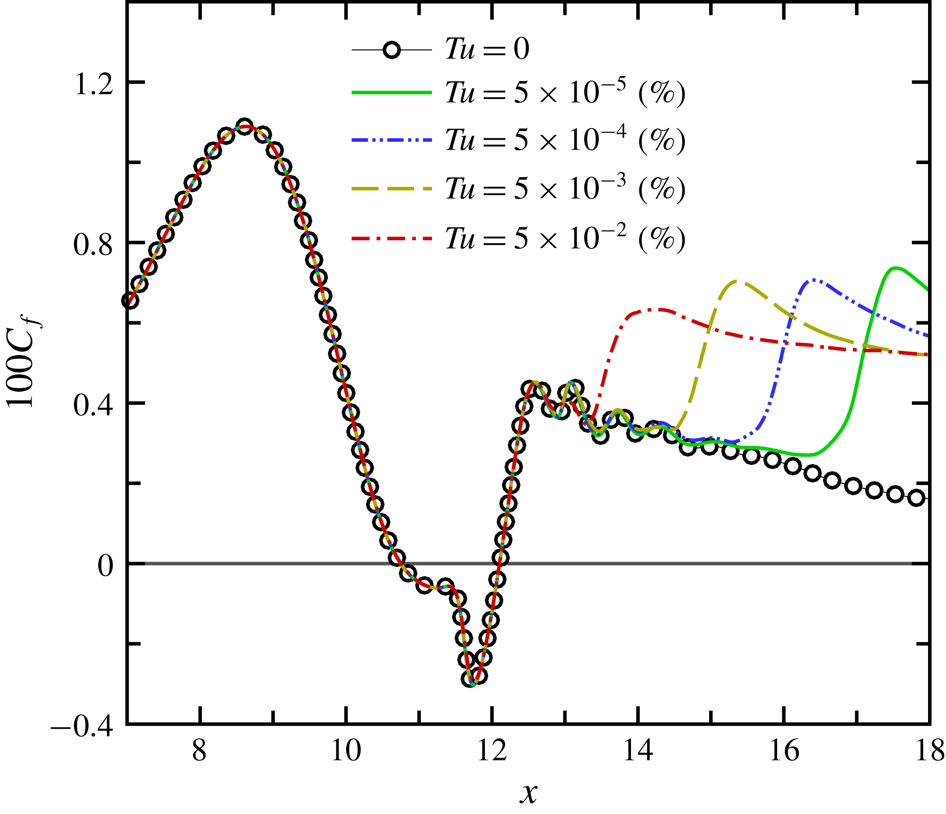
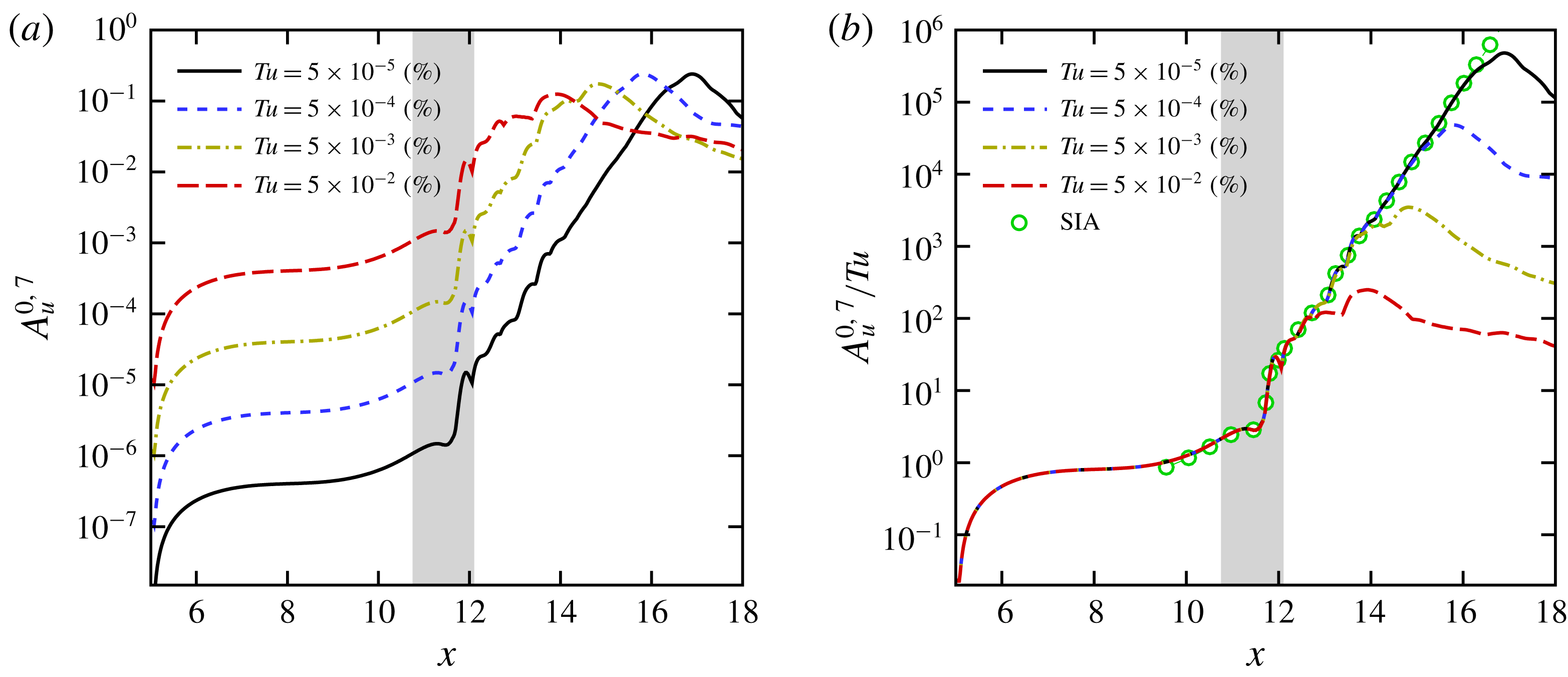
The streamwise development of the time- and spanwise-averaged wall skin-friction coefficient as obtained from DNS is plotted in figure 15 for the controlled flow ( $B=0.01$ ) for various FST intensities. In all cases, the flow separates at $x_{s}=10.76$ and reattaches near $x_{r}=12.1$ leading to virtually identical bubble sizes. It can therefore be concluded that for flow control with $B=0.01$ and the levels of FST investigated here (low FST intensities), the control effectiveness for all cases is solely a consequence of the wall-normal momentum exchange provided by the strong spanwise ‘rollers’ resulting from the control. Despite the same bubble sizes, the boundary-layer development downstream of the mean reattachment location is very different for the various FST intensities. For the highest FST intensity investigated, $Tu=0.05\,\%$ , $c_{f}$ closely follows the laminar curve of the zero FST case until $x=13.2$ from where it grows rapidly due to the laminar-to-turbulent transition. The x-location where the $c_{f}$ starts to deviate from the laminar curve moves downstream when the level of FST decreases. Comparison of the $c_{f}$ distributions for $Tu=0$ and $Tu=5\times 10^{-5}~(\%)$ indicates that the limit of no free-stream turbulence can be reached asymptotically as the level of FST decreases.

In figure 16, a side-by-side comparison of results obtained from the simulations with $Tu=5\times 10^{-2}~(\%)$ and $Tu=5\times 10^{-5}~(\%)$ is presented. Shown are visualizations of instantaneous contours of the spanwise vorticity in the $x$ – $y$ plane (spanwise averaged) and the total vorticity in the $x$ – $z$ plane extracted at $y(x)=1.5\unicode[STIX]{x1D6FF}_{1}(x)$ , where $\unicode[STIX]{x1D6FF}_{1}(x)$ is the local mean displacement thickness. As can be observed in figure 16(a), a spanwise dominant vortex structure that has just been shed from the separated shear layer experiences a strong modulation (‘shredding’) in the lateral direction for a FST intensity of $Tu=5\times 10^{-2}~(\%)$ . In contrast, for extremely low FST amplitude, $Tu=5\times 10^{-5}~(\%)$ , in figure 16(b), the flow remains laminar. The dominant structures remain essentially two-dimensional downstream of the mean reattachment location, which is very similar to the zero FST case (bottom plot in figure 13 a). It is not until much further downstream near the outflow boundary that a slight spanwise modulation (‘shredding’) is visible, which however is considerably less pronounced compared to the $Tu=0.05\,\%$ case.

Figure 15.

Comparison of time- and spanwise-averaged wall skin-friction coefficients of the controlled flow with $B=0.01$ for various levels of FST intensity.

Figure 16.

Instantaneous contours of spanwise-averaged spanwise vorticity in the $x$ – $y$ plane (top) and total vorticity in the $x$ – $z$ plane at $y(x)=1.5\unicode[STIX]{x1D6FF}_{1}(x)$ (bottom) for the controlled flow with $B=0.01$ . (a) $Tu=5\times 10^{-2}~(\%)$ ; (b) $Tu=5\times 10^{-5}~(\%)$ . Dashed red lines indicate the mean separation and reattachment locations.

Figure 17.

(a) Comparison of the downstream development of the K-mode for various FST intensities. Plotted are the wall-normal maximum of $u^{\prime }$ -velocity Fourier amplitude. (b) Data from (a) scaled with the inlet turbulence intensity. Included in (b) is mode $(0,7)$ as obtained from SIA. Shaded area corresponds to the mean separated region.

Finally in figure 17(a), the streamwise evolution of the wall-normal maximum of the $u^{\prime }$ -velocity Fourier amplitude of K-mode, $A_{u}^{0,7}$ , is shown for the various levels of FST. Immediately downstream of the inflow location, the K-mode experiences streamwise growth for $x<6$ , which is most likely the consequence of transient growth and lift-up mechanisms (Landahl Reference Landahl1975). The initial growth of the K-mode is followed by slow streamwise growth in the region of a favourable pressure gradient $6\leqslant x\leqslant 9.6$ . For $x>9.6$ , the onset of the adverse pressure gradient, the K-mode experiences slightly stronger amplification up to the mean reattachment location ( $x\approx 11.6$ ), where it starts to get strongly amplified. Downstream of the mean reattachment location, the K-mode exhibits a nearly constant exponential growth rate until it reaches the peak amplitude, a level close to that of the saturated primary mode, which then triggers the transition to turbulence (see figure 14, left plot for $Tu=0.005\,\%$ ).

As seen in figure 17(a), the streamwise development of the K-mode from the beginning all the way up to the reattachment location, and even further downstream until $x\approx 13$ , is very similar for all the different levels of FST investigated here (just shifted vertically with respect to each other). Therefore, when the disturbance amplitudes are rescaled with the turbulence intensity at the inflow boundary, as shown in figure 17(b), for all FST intensities investigated, the curves collapse up to $x\leqslant 13$ . This is an indication that the growth of the 3-D low-frequency modes caused by the primary wave scale linearly with FST intensity, and that the receptivity mechanism in this region (upstream of the separation location, inside the separated region, and within the secondary instability regime) is linear with regard to the FST intensity. A similar observation was reported by Schrader, Amin & Brandt (Reference Schrader, Amin and Brandt2010) for an attached laminar boundary layer even for higher FST intensities of up to $1\,\%$ . What is remarkable in figure 17(b) is that SIA accurately captures that behaviour from upstream of the separation location and through the separated region almost all the way until the peak amplitude of the K-mode occurs.

For the given forcing amplitude of $B=0.01$ , it can therefore, be concluded that for $Tu\leqslant 6.25\times 10^{-7}~(\%)$ , the boundary layer remains laminar in the entire computational domain similar to the results obtained from the zero FST simulation.

4 Conclusion

The objective of this paper is to answer the question whether the surprising effectiveness of selected 2-D harmonic forcing that can lead to relaminarization and transition delay could also be observed in a realistic wind tunnel operation conditions, i.e. in the presence of free-stream turbulence. Toward this end, high-resolution DNS of canonical separation bubbles on a flat plate were carried out and the response to high-amplitude 2-D forcing was investigated in the absence of and in the presence of FST. Harmonic blowing and suction through a spanwise slot was shown to be very effective in both environments with respect to reducing the extent of separation. This was attributed to the shear-layer instability, which amplifies the disturbance input. Without FST, the controlled flow is virtually two-dimensional and dominated by strong spanwise vortices (‘rollers’). This suggests that the control is effective in suppressing temporally growing disturbances.

When very low-amplitude isotropic turbulence velocity fluctuations, which are generated based on a weighted superposition of the continuous modes of the Orr–Sommerfeld and homogeneous Squire equations, were seeded at the inflow boundary of the computational domain, the situation changed. With even very low FST level, complete relaminarization of the flow within the computational domain as observed in the zero FST case, could no longer be accomplished. In particular, the flow remained laminar only for short distance downstream of the reattachment location until it transitioned to turbulence. This can be explained by the fact that in the presence of even very small levels FST, strong interactions occur between the high-amplitude 2-D disturbance waves introduced by the forcing and 3-D Klebanoff modes that are excited by the FST.

Based on the results presented here, corroborated by instantaneous flow visualizations, spectral analysis, modal decomposition and secondary instability investigations, the transition process for a controlled (forced) LSB subjected to a low level of FST, is governed by the interaction of the primary 2-D wave with the forcing frequency and the steady (very low-frequency) K-mode and unsteady disturbance waves with the forcing frequency and with the same spanwise mode number as the K-mode. Based on the linearized Navier–Stokes equations (without additional assumptions as required by the standard secondary instability analysis) and using time-dependent solutions of DNS as a base flow, secondary instability investigations indicated that the time-periodic, controlled flow is secondarily unstable to broad range of low-frequency 3-D disturbance waves. The SIA investigations have also shown that the spanwise wavelength associated with K-mode is very close to that of the most unstable 3-D disturbances. Therefore, it can be concluded that the K-mode prevails further downstream and dominates the transition process because it has the largest initial amplitude upstream of the separation location among all the 3-D disturbances.

Detailed investigations were carried out to evaluate the effect of the forcing amplitude and FST intensity on the effectiveness of the separation control in general and on the transition process in particular. For all levels of FST and forcing amplitudes investigated, the underlying instability mechanisms leading to transition were similar, in particular regarding the interaction of the 3-D K-mode and the 2-D primary wave. However, the response of the boundary layer with respect to the forcing amplitude and FST intensity were different. For a given level of FST intensity, a reduction in input forcing amplitude increases the bubble size, although the convective instability of the mean flow with respect to 2-D disturbances is increased. Simultaneously, the transition to turbulence is delayed. Two physical mechanisms appear to play the major role in the delay of boundary-layer transition: (i) The onset of the strong growth of low-frequency 3-D modes is moved farther downstream, and (ii) the exponential amplification rate of the K-modes was reduced. On the other hand for a given forcing amplitude, increasing the intensity of the incoming vortical fluctuations (due to increased FST), results in virtually identical bubble sizes independent of FST levels for $Tu\leqslant 0.05\,\%$ . Despite the same bubble sizes, the boundary-layer development downstream of the mean reattachment location was very sensitive to the FST intensity. While the onset of the growth and the subsequent amplification rate of the K-mode was almost identical for the levels of FST intensity examined, laminar-to-turbulent transition occurred further downstream for decreasing levels of FST. This can be explained by the fact that the growth of the 3-D low-frequency modes scale linearly with FST intensity.

In summary, ‘clean’ simulations where the FST is negligible (zero FST) is extremely difficult to accomplish in practical wind tunnel experiments. However, in extremely low FST levels as in free flight, the relaminarization strategy may still be advantageously employed. The presented results are an important finding as they advance our fundamental physical understanding of the effect of FST on the separation and separation control.

Acknowledgements

This work was supported by the Air Force Office of Scientific Research (AFOSR) under grant number FA9550-14-1-0184, with Dr D. R. Smith serving as the program manager.

References

Balzer, W. & Fasel, H. F. 2016 Numerical investigation of the role of free-stream turbulence in boundary-layer separation. J. Fluid Mech. 801, 289–321.Google Scholar

Benton, S. I. & Visbal, M. R. 2016 Investigation of high-frequency separation control mechanisms for delay of unsteady separation. In 8th AIAA Flow Control Conference, AIAA 2016-4241. American Institute of Aeronautics and Astronautics (AIAA).Google Scholar

Brandt, L., Henningson, D. S. & Ponziani, D. 2002 Weakly nonlinear analysis of boundary layer receptivity to free-stream disturbances. Phys. Fluids 14 (4), 1426–1441.Google Scholar

Brandt, L., Schlatter, P. & Henningson, D. S. 2004 Transition in boundary layers subject to free-stream turbulence. J. Fluid Mech. 517, 167–198.Google Scholar

Diwan, S. S. & Ramesh, O. N. 2009 On the origin of the inflectional instability of a laminar separation bubble. J. Fluid Mech. 629, 263–298.Google Scholar

Dong, M. & Wu, X. 2013 On continuous spectra of the Orr–Sommerfeld/Squire equations and entrainment of free-stream vortical disturbances. J. Fluid Mech. 732, 616–659.Google Scholar

Embacher, M. & Fasel, H. F. 2014 Direct numerical simulations of laminar separation bubbles: investigation of absolute instability and active flow control of transition to turbulence. J. Fluid Mech. 747, 141–185.Google Scholar

Fasel, H. F. 2002 Numerical investigation of the interaction of the Klebanoff-mode with a Tollmien–Schlichting wave. J. Fluid Mech. 450, 1–33.Google Scholar

Fransson, J. H., Brandt, L., Talamelli, A. & Cossu, C. 2005 Experimental study of the stabilization of Tollmien–Schlichting waves by finite amplitude streaks. Phys. Fluids 17 (5), 054110.Google Scholar

Gaster, M. 1967 The structure and behaviour of laminar separation bubbles. In ARC, Reports and Memoranda, No. 3595. Aeronautical Research Council.Google Scholar

Goldstein, M. E. 2014 Effect of free-stream turbulence on boundary layer transition. Phil. Trans. R. Soc. Lond. A 372 (2020), 1–18.Google Scholar

Grosch, C. E. & Salwen, H. 1978 The continuous spectrum of the Orr–Sommerfeld equation. Part 1. The spectrum and the eigenfunctions. J. Fluid Mech. 87 (1), 33–54.Google Scholar

Herbert, T. 1988 Secondary instability of boundary layers. Annu. Rev. Fluid Mech. 20 (1), 487–526.Google Scholar

Hosseinverdi, S., Balzer, W. & Fasel, H. F. 2012 Direct numerical simulations of the effect of free-stream turbulence on ‘long’ laminar separation bubbles. In 42th AIAA Fluid Dynamics Conference and Exhibit, AIAA 2012-2972. American Institute of Aeronautics and Astronautics (AIAA).Google Scholar

Hosseinverdi, S. & Fasel, H. F. 2017 Numerical investigation of the interaction of active flow control and Klebanoff modes. In 47th AIAA Fluid Dynamics Conference, AIAA 2017-4419. American Institute of Aeronautics and Astronautics (AIAA).Google Scholar

Huerre, P. & Monkewitz, P. A. 1990 Local and global instabilities in spatially developing flows. Ann. Rev. Fluid Mech. 22 (1), 473–537.Google Scholar

Jacobs, R. G. & Durbin, P. A. 2001 Simulations of bypass transition. J. Fluid Mech. 428, 185–212.Google Scholar

Jones, L. E., Sandberg, R. D. & Sandham, N. D. 2008 Direct numerical simulations of forced and unforced separation bubbles on an airfoil at incidence. J. Fluid Mech. 602, 175–207.Google Scholar

Kendall, J. M. 1985 Experimental study of disturbances produced in a pretransitional laminar boundary layer by weak freestream turbulence. In 18th Fluid Dynamics and Plasma Dynamics and Lasers Conference, AIAA 1985-1695. American Institute of Aeronautics and Astronautics (AIAA).Google Scholar

Kendall, J. M. 1990 Boundary layer receptivity to freestream turbulence. In 21st Fluid Dynamics, Plasma Dynamics and Lasers Conference, AIAA 1990-1504. American Institute of Aeronautics and Astronautics (AIAA).Google Scholar

Klebanoff, P. S. 1971 Effect of free-stream turbulence on a laminar boundary layer. Bull. Am. Phys. Soc. 16 (11), 1323.Google Scholar

Landahl, M. T. 1975 Wave breakdown and turbulence. SIAM J. Appl. Maths 28 (4), 735–756.Google Scholar

Leib, S. J., Wundrow, D. W. & Goldstein, M. E. 1999 Effect of free-stream turbulence and other vortical disturbances on a laminar boundary layer. J. Fluid Mech. 380, 169–203.Google Scholar

Liu, Y., Zaki, T. A. & Durbin, P. A. 2008a Boundary-layer transition by interaction of discrete and continuous modes. J. Fluid Mech. 604, 199–233.Google Scholar

Liu, Y., Zaki, T. A. & Durbin, P. A. 2008b Floquet analysis of secondary instability of boundary layers distorted by Klebanoff streaks and Tollmien–Schlichting waves. Phys. Fluids 20 (12), 124102.Google Scholar

Lumley, J. L. 1967 The structure of inhomogeneous turbulent flows. Atmos. Turbul. Radio Wave Propag. 166–178.Google Scholar

Marxen, O. & Henningson, D. S. 2011 The effect of small-amplitude convective disturbances on the size and bursting of a laminar separation bubble. J. Fluid Mech. 671, 1–33.Google Scholar

Marxen, O., Lang, M. & Rist, U. 2012 Discrete linear local eigenmodes in a separating laminar boundary layer. J. Fluid Mech. 711, 1–26.Google Scholar

Marxen, O., Lang, M., Rist, U. & Wagner, S. 2003 A combined experimental/numerical study of unsteady phenomena in a laminar separation bubble. Flow Turbul. Combust. 71 (1), 133–146.Google Scholar

Marxen, O. & Rist, U. 2010 Mean flow deformation in a laminar separation bubble: separation and stability characteristics. J. Fluid Mech. 660, 37–54.Google Scholar

Meitz, H. L. & Fasel, H. F. 2000 A compact-difference scheme for the Navier–Stokes equations in vorticity–velocity formulation. J. Comp. Phys. 157 (1), 371–403.Google Scholar

Morkovin, M. V., Reshotko, E. & Herbert, T. 1994 Transition in open flow systems: a reassessment. Bull. APS 39 (9), 1–31.Google Scholar

Postl, D., Balzer, W. & Fasel, H. F. 2011 Control of laminar separation using pulsed vortex generator jets: direct numerical simulations. J. Fluid Mech. 676, 81–109.Google Scholar

Rempfer, D. & Fasel, H. F. 1994 Evolution of three-dimensional coherent structures in a flat-plate boundary layer. J. Fluid Mech. 260, 351–375.Google Scholar

Ricco, P., Luo, J. & Wu, X. 2011 Evolution and instability of unsteady nonlinear streaks generated by free-stream vortical disturbances. J. Fluid Mech. 677, 1–38.Google Scholar

Rodríguez, D., Gennaro, E. M. & Juniper, M. P. 2013 The two classes of primary modal instability in laminar separation bubbles. J. Fluid Mech. 734, R4-1–R4-11.Google Scholar

Rodríguez, D. & Theofilis, V. 2010 Structural changes of laminar separation bubbles induced by global linear instability. J. Fluid Mech. 655, 280–305.Google Scholar

Schrader, L. U., Amin, S. & Brandt, L. 2010 Transition to turbulence in the boundary layer over a smooth and rough swept plate exposed to free-stream turbulence. J. Fluid Mech. 646, 297–325.Google Scholar

Schubauer, G. B. & Skramstad, H. K.1948 Laminar-boundary-layer oscillations and transition on a flat plate. NACA Tech. Rep. 909.Google Scholar

Sirovich, L. 1987 Turbulence and the dynamics of coherent structures. I. coherent structures. Q. Appl. Maths 45 (3), 561–571.Google Scholar

Spalart, P. R. & Strelets, M. K. 2000 Mechanisms of transition and heat transfer in a separation bubble. J. Fluid Mech. 403, 329–349.Google Scholar

von Terzi, D. A.2004 Numerical investigation of transitional and turbulent backward-facing step flows. PhD thesis, The University of Arizona.Google Scholar

Wu, X. & Dong, M. 2016 Entrainment of short-wavelength free-stream vortical disturbances in compressible and incompressible boundary layers. J. Fluid Mech. 797, 683–728.Google Scholar

Figure 1.(a) Uncontrolled flow: instantaneous contours of $\unicode[STIX]{x1D714}_{z}$-vorticity together with the contour lines of $\ln |\unicode[STIX]{x1D714}_{z}|$ for zero FST (top) and FST of $Tu=0.005\,\%$ (bottom). (b) Contours of the longitudinal component of the normal Reynolds stress, $\overline{u^{\prime }u^{\prime }}$, at $x=9.5$ for $Tu=0.005\,\%$. The overbar represents the time average. The mean separation and reattachment locations are marked by up arrows in (a).

Figure 2.Spanwise one-dimensional energy spectra of the streamwise velocity at selected streamwise stations for the uncontrolled flow with $Tu=0.005\,\%$. Dashed lines are the displacement thickness. The wall-normal coordinate was normalized with the local boundary-layer thickness.

Figure 3.Instantaneous flow visualization for controlled flow. Plotted are iso-surfaces of $\unicode[STIX]{x1D706}_{2}=-40$ coloured by u-velocity in perspective view together with the contours of $\unicode[STIX]{x1D714}_{z}$-vorticity and contour lines of $\ln |\unicode[STIX]{x1D714}_{z}|$ in the $x$–$y$ plane (spanwise averaged). (a) zero FST; (b) $Tu=0.005\,\%$.

Figure 4.(a) Comparison of skin-friction coefficients for controlled flow. (b) Time-averaged contours of the spanwise wall vorticity (top–down view) of controlled flow for zero FST (top) and $Tu=0.005\,\%$ (bottom). Dashed lines represent $\overline{\unicode[STIX]{x1D714}}_{z}=0$.

Figure 5.Wall-normal u-velocity profiles at $x=15$ for the controlled case with $B=0.05$. (a) u-velocity profiles at five time instances separated by one fifth of the forcing period ($T_{hbs}$) shown together with the time-averaged profile for zero FST case. (b) Comparison of the time-averaged u-velocity profile for zero FST and $Tu=0.005\,\%$.

Figure 6.Disturbance development of the Fourier amplitudes of controlled flow with $Tu=0.005\,\%$. (a) Steady disturbance waves. (b) Unsteady modes with the forcing frequency. The vertical dashed lines correspond to the forcing location and shaded area represents the mean separated region. Also, $(0,7)-UNC$ in (a) and $(1,7)-UNC$ in (b) refer to the steady and unsteady K-modes for the uncontrolled flow with FST, respectively, and $(1,0)-Tu=0$ in (b) corresponds to the primary wave for controlled flow with zero FST.

Figure 7.POD eigenvalue (energy) spectrum for the controlled flow with $Tu=0.005\,\%$: (a) normalizied POD eigenvalues and (b) their cumulative energy. Spatial eigenfunctions and time signal of coloured symbols in (a) are shown in figures 8 and 9.

Figure 8.Dominant POD eigenfunctions for the controlled LSB with $B=0.05$ and $Tu=0.005\,\%$. Shown are iso-surfaces of $|u|=0.4$. Dashed red lines indicate the mean separation and reattachment locations.

Figure 9.(a) POD time coefficients of modes 1 (red), 3 (green), 5 (black), 6 (purple), 7 (dark yellow) and 9 (blue). (b) Associated frequency spectra. Controlled LSB with $B=0.05$ in the presence of FST with $Tu=0.005\,\%$.

Table 1.Computational parameters used to define the volume force in (3.7).

Figure 10.Comparison of local spatial growth rates (top) and wall-normal distributions of the $u^{\prime }$-velocity Fourier amplitudes at several x-locations (bottom) obtained from SIA and DNS with $Tu=0.005\,\%$: (a) mode $(0,7)$; (b) mode $(1,7)$. Disturbance amplitudes are scaled by their respective maximum. Dashed lines in the bottom plots represent the corresponding time-averaged $u$-velocity profile normalized by the edge velocity. LINTAB in (a) refers to linear calculation for mode (0,7) based on the time-averaged base flow. Shaded area indicates the mean separated region. Wall-normal coordinates are normalized by the local boundary-layer thickness.

Figure 11.Results from the secondary instability analysis of the controlled flow with $B=0.05$ for steady disturbances. (a) Growth rate ($\unicode[STIX]{x1D70E}$) of disturbances as a function of spanwise wavelength where $\unicode[STIX]{x1D70E}_{1}$ corresponds to the averaged $\unicode[STIX]{x1D70E}$ over $11\leqslant x\leqslant 12.5$, and $\unicode[STIX]{x1D70E}_{2}$ represents the exponentially fitted $\unicode[STIX]{x1D70E}$ for $x>12.5$. (b) Variation of energy growth ratio versus spanwise wavelength. The spanwise wavelength of the K-mode, $\unicode[STIX]{x1D706}_{z,K}$, is marked by vertical dashed lines.

Figure 12.(a) Streamwise development of the K-mode obtained from SIA for controlled flow with different forcing amplitudes $B$. (b) Mean separation/reattachment locations ($x_{s}$, $x_{r}$) as well as onset locations of K-mode growth ($x_{K}$) as a function of $\log (B)$. Right vertical axis in (b) is the exponential growth rate of the K-mode measured downstream of $x_{r}$.

Figure 13.(a) Instantaneous contours of the spanwise-averaged spanwise vorticity and contour lines (blue dashed) of $\ln (|\unicode[STIX]{x1D714}_{z}|)$ for different forcing amplitudes with $Tu=0.005\,\%$. From top to bottom: $B=0.05$, $B=0.025$ and $B=0.01$. The bottom plot was obtained from a zero FST simulation with $B=0.01$. (b) Perspective view of instantaneous flow visualization for the case with $B=0.01$. Plotted are iso-surfaces of $\unicode[STIX]{x1D706}_{2}=-40$ coloured by $u$-velocity.

Figure 14.Streamwise development of primary wave, $(1,0)$, and K-mode, $(0,7)$, for different forcing amplitudes. Shown also is the streamwise amplitude development for modes $(1,0)$ and $(0,7)$ computed with LINTAB (time-averaged base flow) and SIA (time-dependent base flow) for mode $(0,7)$. The mean separated region is identified by shaded area.

Figure 15.Comparison of time- and spanwise-averaged wall skin-friction coefficients of the controlled flow with $B=0.01$ for various levels of FST intensity.

Figure 16.Instantaneous contours of spanwise-averaged spanwise vorticity in the $x$–$y$ plane (top) and total vorticity in the $x$–$z$ plane at $y(x)=1.5\unicode[STIX]{x1D6FF}_{1}(x)$ (bottom) for the controlled flow with $B=0.01$. (a) $Tu=5\times 10^{-2}~(\%)$; (b) $Tu=5\times 10^{-5}~(\%)$. Dashed red lines indicate the mean separation and reattachment locations.

Figure 17.(a) Comparison of the downstream development of the K-mode for various FST intensities. Plotted are the wall-normal maximum of $u^{\prime }$-velocity Fourier amplitude. (b) Data from (a) scaled with the inlet turbulence intensity. Included in (b) is mode $(0,7)$ as obtained from SIA. Shaded area corresponds to the mean separated region.

Article contents

Role of Klebanoff modes in active flow control of separation: direct numerical simulations

Abstract

JFM classification

Information

1 Introduction

2 Computational framework

2.1 Simulation set-up

2.2 Free-stream turbulence generation

2.3 Flow control: harmonic blowing and suction through a 2-D slot

3 Results

3.1 Main features of uncontrolled flow

3.2 Characteristic features of controlled flow

3.2.1 Disturbance evolution

3.2.2 Proper orthogonal decomposition

3.2.3 Secondary instability investigations

3.3 Effect of forcing amplitude

3.4 Effect of free-stream turbulence level

4 Conclusion

Acknowledgements

References

Save article to Kindle

Save article to Dropbox

Save article to Google Drive

Reply to: Submit a response

Your details

You have entered the maximum number of contributors

Conflicting interests