Introduction
The fossil record provides unique information about the history of biodiversity on Earth, yielding insights into mass extinction events and other episodes of turnover that would not be recognized solely from the study of extant species. However, inferring patterns of diversity and the dynamics of speciation and extinction from the fossil record is beset with difficulties, not least those resulting from the heterogeneous sampling of fossil specimens through time and space. This heterogeneity is caused by a diverse array of sampling biases, including the spatial and temporal architecture of the rock record itself (geological biases) and the way the rock record has been sampled by paleontologists (anthropogenic biases) (Raup Reference Raup1972; Smith 2001; Smith and McGowan Reference Smith and McGowan2011). Various quantitative methods have been developed to compensate for these biases and may be effective when sufficiently rich databases of fossil occurrences are available (e.g., Alroy Reference Alroy1996, 2009, Reference Alroy2014; Foote and Sepkoski Reference Foote and Sepkoski1999; Foote Reference Foote2000; Silvestro et al. Reference Silvestro, Salamin and Schnitzler2014).
The temporal resolution (i.e., the fineness of stratigraphic divisions used in discrete-time analyses) of paleobiological studies of diversification is limited by the typical resolution at which fossil occurrences are reported in databases. For example, in the Paleobiology Database (http://paleodb.org), which is widely used in global-scale paleobiological studies (e.g., Alroy et al. Reference Alroy, Marshall, Bambach, Bezusko, Foote, Fürsich, Hansen, Holland, Ivany, Jablonski, Jacobs, Jones, Kosnik, Lidgard, Low, Miller, Novack-Gottshall, Olszewski, Patzkowsky, Raup, Roy, Sepkoski, Sommers, Wagner and Webber2001; Wagner et al. Reference Wagner, Kosnik and Lidgard2006; Hannisdal and Peters Reference Hannisdal and Peters2011; Mayhew et al. Reference Mayhew, Bell, Benton and McGowan2012), fossil occurrences are typically assigned to the scale of Phanerozoic stages (mean 6.2 Myr) or substages (mean 3.5 Myr). Sepkoski’s older, but nonetheless highly influential, databases of Phanerozoic marine macrofossils resolve over half their genera to substage-level temporal units (mean 3.51 Myr; Sepkoski Reference Sepkoski1982, Reference Sepkoski2002). However, the coarse time resolution of these global fossil databases can result in aliasing, and exaggeration of standing diversity estimates due to the conflation of the ranges of non-overlapping taxa into one bin; this limits our ability to make inferences about short-lived events in the evolution of biodiversity. Such events include mass extinctions and their subsequent recovery episodes, which could potentially take place on shorter timescales (e.g., Twitchett et al. Reference Twitchett, Krystyn, Baud, Wheeley and Richoz2004; Smith and Botha-Brink Reference Smith and Botha-Brink2014; Wilson Reference Wilson2014) or within time bins. This error is most clearly evident in studies of the Cretaceous/Paleogene mass extinction event: although it certainly resulted in catastrophic reductions in species diversity in its immediate aftermath, subsampled richness estimates for both marine and terrestrial fossils at the level of a geological stage (4.4 Myr=earliest Paleogene Danian stage) actually increase across this boundary (Alroy et al. Reference Alroy, Aberhan, Bottjer, Foote, Fürsich, Harries, Hendy, Holland, Ivany, Kiessling, Kosnik, Marshall, McGowan, Miller, Olszewski, Patzkowsky, Peters, Villier, Wagner, Bonuso, Borkow, Brenneis, Clapham, Fall, Ferguson, Hanson, Krug, Layou, Leckey, Nürnberg, Powers, Sessa, Simpson, Tomašových and Visaggi2008; Benson et al. Reference Benson, Butler, Alroy, Mannion, Carrano and Lloyd2016; Close et al. Reference Close, Benson, Upchurch and Butler2017). This illustrates how the use of data resolved only to coarse time bins allows a recovery of species richness to greater than pre-extinction levels within a few million years to entirely overwrite the signal of low postextinction richness.
High-resolution databases of fossil occurrence can provide greater temporal resolution, substantially helping to resolve the timing and magnitude of key turnover events in the history of life on Earth. The latest Cretaceous and Cenozoic fossil records of North American land mammals provide a model example of the power of this type of study (e.g., Alroy Reference Alroy2009; Quental and Marshall Reference Quental and Marshall2013), as well as considerable insight into patterns of evolution both during, and after, the Cretaceous/Paleogene mass extinction event (Wilson Reference Wilson2014; Longrich et al. Reference Longrich, Scriberas and Wills2016). However, few other examples exist, especially for the continental fossil record (which is relatively poorly sampled compared with the marine fossil record) and for pre-Cenozoic events (the relatively recent Cenozoic record is richer and stratigraphically more finely resolved).
The Capitanian (“end-Guadalupian”) mass extinction provides a second example of how coarse stratigraphic resolution can obscure the dynamics of turnover inferred from fossil data. This was initially considered part of the end-Permian mass extinction due to lack of evidence for “background” extinction rates between the Guadalupian and Lopingian [Dzhulfian] (Raup and Sepkoski Reference Raup and Sepkoski1982), but a reevaluation at higher temporal resolution recognized the “end-Guadalupian” extinction event as a separate crisis that is potentially one of the most severe in metazoan history (Stanley and Yang Reference Stanley and Yang1994). Subsequent quantitative analyses of turnover rates in the Phanerozoic record of marine invertebrates have mostly considered the Guadalupian (duration=~13 Myr) as a single interval and initially supported an extinction peak in this interval (e.g., Sepkoski Reference Sepkoski1996; Bambach et al. Reference Bambach, Knoll and Wang2004). However, many more recent studies have tended to downplay Capitanian extinction intensity, especially compared with other mass extinction events (Alroy Reference Alroy2008 [mean interval duration=11.3 Myr], 2010b [= 10.8 Myr], 2014 [=10 Myr]; Foote Reference Foote2003 [7.4 Myr for stages or 3.5 Myr if resolved to substage]; Clapham et al. Reference Clapham, Shen and Bottjer2009 [standardized for interval duration but 10.2 Myr for Guadalupian]; Payne and Clapham Reference Payne and Clapham2012 [13.5 Myr]; McGhee et al. Reference McGhee, Clapham, Sheehan, Bottjer and Droser2013 [13.5 Myr]). The study of Stanley (Reference Stanley2016) is an exception to this; by accounting for singletons and the backward smearing of extinctions due to the Signor-Lipps effect, he determined the Capitanian mass extinction (his Guadalupian crisis) to be only slightly less severe than the Cretaceous/Paleogene mass extinction event. Stanley (Reference Stanley2016) also suggested that the comparatively greater extinction intensity at the end-Permian event (approximately 8 Myr later) may have been exacerbated by an only partial recovery from Capitanian extinction event by this time.
The lack of consistency among appraisals of the severity of extinction in the Capitanian may be partly the result of its occurrence within a geochronological stage rather than at a stage boundary, as is suggested by several studies of fossiliferous sections in southeastern China and in Spitsbergen, at least for foraminiferans (Bond et al. Reference Bond, Hilton, Wignall, Ali, Stevens, Sun and Lai2010; Bond and Wignall Reference Bond and Wignall2014; Bond and Grasby Reference Bond and Grasby2017). This could limit the ability for some analyses at the stage level to recognize a mass extinction, as rapid recovery could obscure a dramatic loss of diversity. More broadly, it is a symptom of the high degree of variability in current statistical treatments of global fossil data sets; so far they have failed to reach consensus on all but the most severe (“big five”) global diversity crises.
Despite continuing disagreement over the broader taxonomic severity of the Capitanian extinction event, field-based studies of marine sections, predominantly in China, suggest that it is closely associated with volcanism in the Emeishan Large Igneous Province and its timing can be constrained to the mid-to-late Capitanian within a window of perhaps 3 Myr (Bond and Wignall Reference Bond and Wignall2014; Bond et al. Reference Bond, Wignall, Joachimski, Sun, Savov, Grasby, Beauchamp and Blomeier2015; Huang et al. Reference Huang, Cawood, Hou, Yang, Ni, Du, Yan and Wang2016; Bond and Grasby Reference Bond and Grasby2017). Furthermore, regional and clade-specific studies suggest that the Capitanian was associated with elevated extinction rates and/or diversity loss in several higher taxa, including ammonoids, brachiopods, conodonts, benthic foraminifera, and brachiopods, as well as reef-building organisms such as sponges, rugose corals, and calcareous algae (Shen and Shi Reference Shen and Shi1996, 2002, Reference Shen and Shi2009; Wang and Sugiyama Reference Wang and Sugiyama2000; Weidlich Reference Weidlich2002; Jin et al. Reference Jin, Shen, Henderson, Wang, Wang, Wang, Cao and Shang2006; Leonova Reference Leonova2009; Bond et al. Reference Bond, Hilton, Wignall, Ali, Stevens, Sun and Lai2010, Reference Bond, Wignall, Joachimski, Sun, Savov, Grasby, Beauchamp and Blomeier2015; Kiessling and Simpson Reference Kiessling and Simpson2011).
Terrestrial turnover estimates for the Permian and Early Triassic have been more limited, relying mostly on ratios of within-bin extinctions and originations to assemblage- or stage-level tallies of taxa derived primarily from the fossil records of the Fore-Ural Basin of European Russia and the Main Karoo Basin of South Africa (Benton Reference Benton1985; Maxwell Reference Maxwell1992; Benton et al. Reference Benton, Tverdokhlebov and Surkov2004, Reference Benton, Ruta, Dunhill and Sakamoto2013; Lucas Reference Lucas2009). Successive tetrapod assemblages of the mid–late Permian in these regions are well studied and form the basis of assemblage zones (South Africa), or simply faunal assemblages (Russia), with durations of 1–5 Myr (e.g., Rubidge Reference Rubidge1995b; Golubev Reference Golubev2000; Arefiev et al. Reference Arefiev, Golubev, Karasev, Zhokina-Naumcheva, Balabanov, Minikh, Minikh, Molostovskaya and Yaroshenko2015; Day et al. Reference Day, Ramezani, Bowring, Sadler, Erwin, Abdala and Rubidge2015b). Most previous analyses of diversity and turnover in Permo-Triassic tetrapods have used these relatively coarse stratigraphic units (but see Materials and Methods for exceptions). They have therefore been unable to recognize patterns of extinction, diversity, and origination associated with short-lived events such as the Capitanian extinction.
The exceptional continuity and density of tetrapod fossil occurrences in the Karoo Basin has occasionally been used to derive high-resolution turnover estimates from more detailed stratigraphic ranges of taxa, especially around the Permo-Triassic boundary (Modesto et al. Reference Modesto, Damiani, Neveling and Yates2003; Smith and Botha Reference Smith and Botha2005; Botha and Smith Reference Botha and Smith2006). Some attention has also been paid to the mid–late Permian transition (between the Tapinocephalus and Pristerognathus Assemblage Zones [AZs]) (Retallack et al. Reference Retallack, Metzger, Greaver, Jahren, Smith and Sheldon2006; Day et al. Reference Day, Ramezani, Bowring, Sadler, Erwin, Abdala and Rubidge2015b), which was associated with a mass extinction among tetrapods that notably exterminated the abundant and widespread Guadalupian therapsid clade Dinocephalia (Lucas Reference Lucas1998, Reference Lucas2009). However, these preliminary appraisals have left key questions unanswered, such as the interplay of extinction and origination (evolution dynamics) surrounding the Capitanian extinction event, the duration of a possible period of low standing richness following it (see Irmis and Whiteside Reference Irmis and Whiteside2011), and especially the extent to which the apparent severity and timing of the Capitanian extinction event might be influenced by nonuniform sampling of fossils through the sequence.
This knowledge gap results from the fact that, although high-resolution analyses have considerable power to resolve the dynamics of origination and extinction on short timescales, they are still subject to the same biases as large-scale studies. In other words, bias results from uneven sampling of stratigraphic packages, even at high resolution. High-resolution studies of turnover and standing diversity in the Karoo Basin so far have not used methods that correct species richness estimates, or rates of origination and extinction, for variation in sampling rate or sample coverage. But studies at coarser time resolutions using Karoo fossil data sets or “global” data sets (of which Karoo fossils form a substantial part) have shown that sampling can strongly influence interpretations of the fossil record, necessitating quantitative approaches that specifically account for this bias (e.g., Irmis and Whiteside Reference Irmis and Whiteside2011; Fröbisch Reference Fröbisch2013, Reference Fröbisch2014).
To explore these questions, we use moving-window estimates of extinction and origination rates and coverage-based subsampling methods (Alroy Reference Alroy2008, Reference Alroy2010a, Reference Alroy2014) to elucidate evolutionary dynamics among terrestrial vertebrates through the mid–late Permian transition in the Karoo Basin. Our analyses were based on a stratigraphically high-resolution database of tetrapod occurrences modified from Day et al. (Reference Day, Ramezani, Bowring, Sadler, Erwin, Abdala and Rubidge2015b). This study represents the first application of robust, sample standardization methods to high-resolution occurrence data for pre-Cenozoic tetrapods.
Materials and Methods
Tetrapod Fossil Data Set
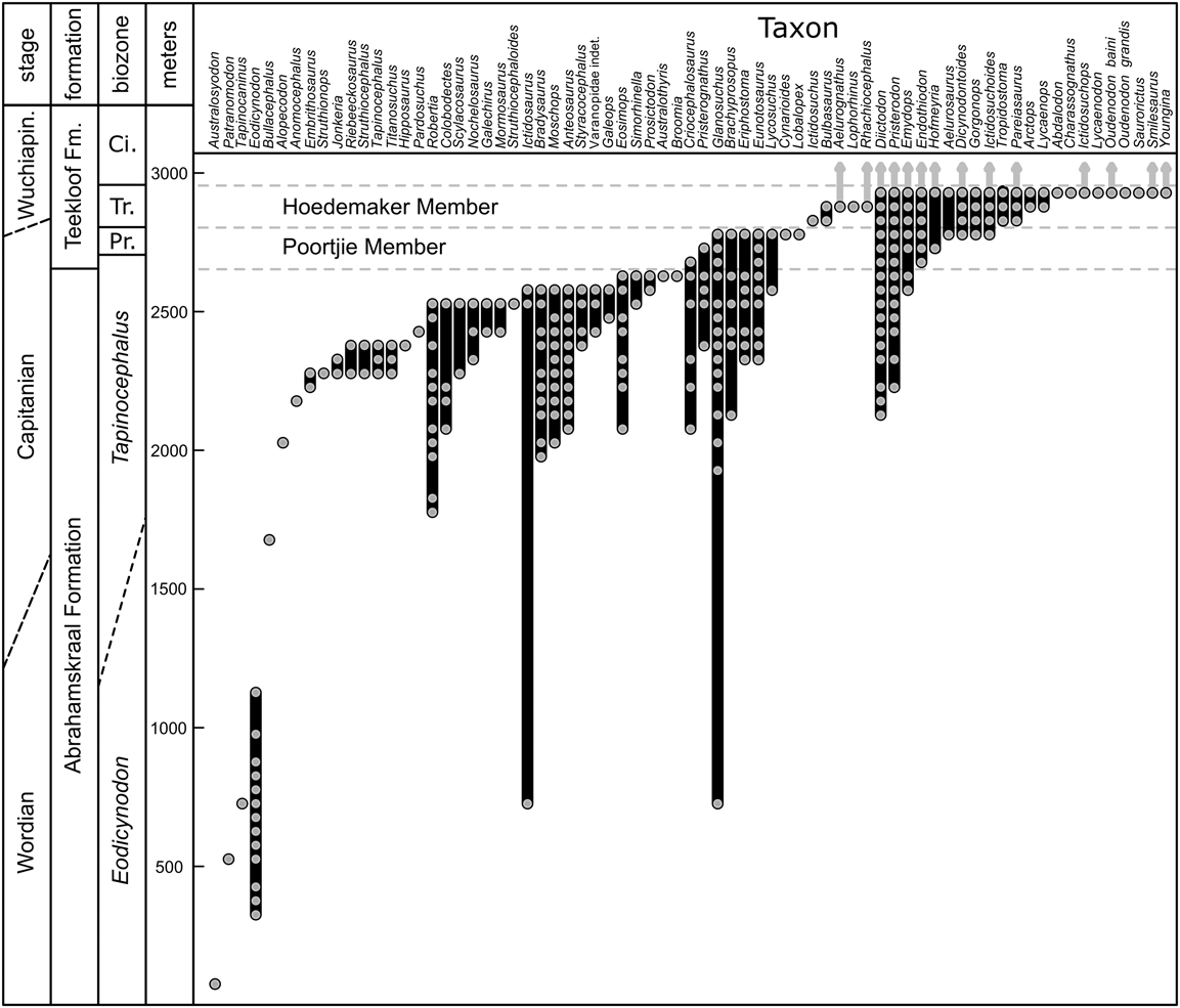
The starting point for the study was a data set of 3067 fossil stratigraphic occurrences (= specimens) within the Abrahamskraal and lower Teekloof Formations of the Beaufort Group (see Fig 1). This builds upon that used by Day et al. (Reference Day, Ramezani, Bowring, Sadler, Erwin, Abdala and Rubidge2015b) but has been expanded by over 50% and benefits from improved stratigraphic accuracy resulting from additional fieldwork (see Supplementary Table 1 for subset of data used here). Fossil taxa are entered as genera when those genera are monospecific in South Africa, and otherwise as species. The database therefore documents species-level occurrences at best. Although specifically and generically indeterminate fossil occurrences are included in the database, they were not included in most of our analyses (described below). One exception to this concerns our use of even specifically indeterminate specimens of varanopid synapsids as a single unit of analysis. We justify this because varanopids are likely represented in South Africa by only one species: Heleosaurus scholtzi (Reisz and Modesto Reference Reisz and Modesto2007). Each fossil occurrence within the Abrahamskraal Formation is assigned to one 50 m stratigraphic bin (or more when there is uncertainty about the position of the locality) over a stratigraphic distance exceeding 2000 m. Specimens from the overlying Poortjie Member of the Teekloof Formation are assigned to either the lower, middle, or upper part of that member (each of which may vary between 40 and 60 m across the outcrop area of the member).
Stratigraphic range chart (black lines) with occurrences (gray disks) of tetrapod species (mostly as monotypic genera) for the Eodicynodon–Tropidostoma assemblage zones (AZs) in the Karoo Basin of South Africa. This range chart makes use of all non-questionable species occurrences (i.e., those not marked with “?”), plus all occurrences of Endothiodon and Glanosuchus (even those marked with “?,” explained in text) for which the stratigraphic position had been checked by M.O.D., either at outcrop or by investigation using geological maps. Uncertainty over the stratigraphic ranges of individual specimens was resolved by placing specimens randomly into one bin in its range of possible positions, as long as this overlapped with the known range of that taxon as determined by better constrained occurrences. If its range of possible positions fell entirely outside the known range, then it was determined to occur in the most proximal bin, and the known range of the taxon was extended to this point. This figure shows only one such iteration, but others are highly similar. Taxa occurring above the studied interval (continuers) are indicated with an ascending gray arrow. Ci., Cistecephalus; Pr., Pristerognathus; Tr., Tropidostoma; Wuchiapin., Wuchiapingian.

The data set incorporates most of the specimens that have been collected from the mid/late Permian boundary interval in South Africa, but is continuously expanding and so is not exhaustive. Most specimens belong to South African collections; however, important specimens, particularly holotypes, from foreign repositories are also included where possible. The original specimen occurrence list (Nicolas Reference Nicolas2007), of which many have poorly constrained stratigraphic origins, assigned occurrences only to the biozone level, and more accurate stratigraphic provenance was only determined later as part of a second Ph.D. thesis (Day Reference Day2013). The original occurrence list also has been substantially bolstered by recent collecting work conducted by the ESI (Evolutionary Studies Institute, Johannesburg) that, over the past decade of field expeditions, has collected more than 625 additional specimens (~20% of the total) with highly accurate stratigraphic provenance from the interval of interest. Specimen identifications were brought up to date as far as possible by incorporating re-identifications provided to collections managers by visiting researchers, from the literature, or by reexamination by one of the authors (M.O.D. or C.F.K.).
Not all of the 3067 fossil specimen occurrences were suitable for analysis. First, we removed specimens for which reliable identifications were not available, which included specimens that could not be identified to the level of genus (e.g., “Therocephalia indet.,” “Scylacosauridae indet.”), and those that had not been recently reappraised by us or in the published literature. To observe differences when only the best-quality data were considered, we also excluded all tentatively identified specimens, with the exception of “?Glanosuchus” and “?Endothiodon.” These latter identifications were deemed to be likely correct, the former due to the historical tendency to assign early therocephalian fossils to the genus Pristerognathus (meaning that identifications as Glanosuchus are more than merely the “default” and generally recognize the uniquely robust cranial morphology of this taxon relative to coeval scylacosaurids), and the latter due to the ready recognizability of Endothiodon based on limited remains (the dental morphology of this taxon is unique among therapsids, permitting even jaw fragments to be confidently identified). The remaining 1031 specimens form our base data set (Supplementary Table 1) and were used to produce a revised stratigraphic-range chart for tetrapods during the mid–late Permian transition in the Karoo Basin (Fig. 1). Of these specimens, almost half (492) belong to a single taxon, the dicynodont Diictodon.
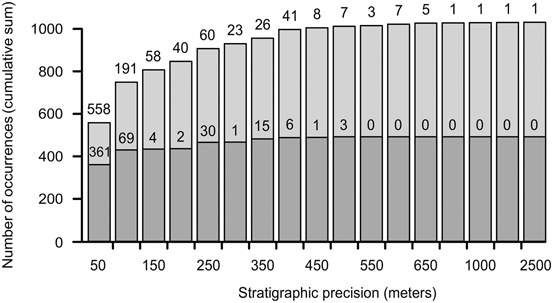
Review of the precision of stratigraphic assignments of these occurrences indicates that slightly more than half (N=558) are assigned precisely to a single 50 m stratigraphic interval (Fig. 2). Others are assigned less precisely, and we excluded specimens that could not be constrained to 3 bins (i.e., 150 m) or fewer. Those occurrences with uncertain provenance that remained (i.e., those that could be constrained to two or three bins) were randomly assigned to one of the 50 m bins within their range of possible positions, considering only bins that fell within the known range of those taxa. We performed this 1000 times, and analyses were conducted on each of these resampled data sets at thresholds of 50 m (only specimens assigned with certainty to a single interval; N=558), 100 m (two intervals; N=749), and 150 m (three intervals, N=807 occurrences).
Precision of stratigraphic assignment to 50 m bins, displayed cumulatively from most accurate (1 bin certainty [= 50 m]) to least accurate (50 bins [= 2500 m]). Numbers above bars indicate total occurrences within bins, both with and without Diictodon. Dark gray portion of bar indicates proportion of cumulative occurrences that are Diictodon.

Day et al. (Reference Day, Ramezani, Bowring, Sadler, Erwin, Abdala and Rubidge2015b) originally divided the Main Karoo Basin into geographic “sectors,” each of which was associated with a local stratigraphic section, to compensate for differences in local thickness of the Abrahamskraal Formation (which varies from 100 m in the south to >2500 m in the north; Day and Rubidge Reference Day and Rubidge2014). The Abrahamskraal Formation was divided into 50 m bins within each sector and was then treated separately. This was appropriate for the application of constrained optimization (CONOP), as this approach considers the sequence of first- and last-appearance events of taxa from observed occurrences in multiple sections. This sequence is then used to create a composite sequence of events independent of any one stratigraphic section (Sadler et al. Reference Sadler, Kemple and Kooser2008). Estimates of origination and extinction rates (using boundary crossers and gap-filler methods) instead use occurrences of taxa within time bins, which in the case of the Karoo must be approximated by stratigraphic bins. For this, a single composite stratigraphic section was required. To achieve this, rates of deposition were postulated to be relatively uniform throughout the southwestern Main Karoo Basin, and a composite section was created by aligning the column of stratigraphic bins from each sector down from the base of the Teekloof Formation (a broadly time-equivalent horizon throughout the basin based on radiometric tuff ages and biostratigraphy; see Day et al. Reference Day, Ramezani, Bowring, Sadler, Erwin, Abdala and Rubidge2015b).
This assumption could be challenged, because the Main Karoo Basin is a flexural foreland basin in which areas at different distances from the orogen experienced different rates of deposition (see Catuneanu et al. Reference Catuneanu, Hancox and Rubidge1998), and the Abrahamskraal Formation is known to become considerably thinner distally (Cole and Wipplinger Reference Cole and Wipplinger2001; Day and Rubidge Reference Day and Rubidge2014). However, as it is the base of the Abrahamskraal Formation that has been shown to be diachronous in the southwest of the basin, much of the difference in thickness is likely due to the later onset of nonmarine deposition in distal areas (e.g., Rubidge et al. Reference Rubidge, Modesto and Sidor1999). Furthermore, the vast majority of specimens from the northern Fraserburg and Victoria West districts are from the Pristerognathus and Tropidostoma AZs, which crop out in the southern portion of those districts in a relatively narrow band. Thus, the effect of variable depositional rates is likely to be limited for these zones. Error from differential rates of deposition may result when incorporating occurrences from the northwestern-most Tapinocephalus AZ, away from the exposure of the Teekloof Formation, but these are relatively few (<10 specimens). The presence of the dicynodont Diictodon (SAM-PK-K5838) close to the base of the Abrahamskraal Formation 45 km northeast of core QU1/65 (Abrahamskraal Fm=500 m; Day and Rubidge Reference Day and Rubidge2014) suggests that these strata all fall within the upper 450 m of the Abrahamskraal Formation as exposed farther south (the range of Diictodon there) and thus, even with continued thinning, the difference in time represented by each 50 m bin does not exceed one or two bins for the informative part of the stratigraphic sequence. Any specimens from the Philippolis and Fauresmith districts of the Free State Province were excluded, as these areas are situated in the midbasin region, much farther north and more distal than other mid-Permian occurrences. Not only has it not been possible to trace lithostratigraphic units this far, but the faunal assemblage displays a unique character and therefore cannot at present be reliably correlated with the southwestern sequences (M.O.D. personal observation).
Our data set is restricted to the Abrahamskraal Formation and lower Teekloof Formation (Poortjie Member). However, data from at least two stratigraphic bins above the final interval of interest are required to estimate origination and extinction rates using the gap-filler method. This requirement could be very limiting on the duration of the informative upper part of the data series (Alroy Reference Alroy2014; this is also true for “three-timer” rate estimates). Therefore, to extend the upper range of the data series, we added data from three additional stratigraphic bins above the Poortjie Member: the lower, middle, and upper parts of the overlying Hoedemaker Member of the Teekloof Formation. Because the Hoedemaker Member is similar in thickness to the Poortjie Member, these bins also reflect ~40–60 m of stratigraphic thickness. These data were based on the counts of occurrences provided by Smith et al. (Reference Smith, Rubidge and Van der Walt2012) for the Tropidostoma AZ, which corresponds in the most part with the Hoedemaker Member. In total, this resulted in the addition of 2649 specimens to the effective data set.
The distribution of taxa within the three bins was determined by retrieving more specific stratigraphic information from publications (for recently revised taxa) and by inference from geological maps and field observation. For common taxa for which no observation exists in the literature (e.g., Tropidostoma), we assumed an even distribution of occurrences across the three bins (see Supplementary Table 1). Although this treatment is less thorough than our treatment of the underlying stratigraphic units, it affects mainly common taxa; most occurrences of rarer taxa have their localities and stratigraphic provenance described in the literature. We consider that the assignments sufficiently represent the occurrence of taxa within the Hoedemaker Member to determine the patterns of taxon survival (from preceding bins) that are used to infer extinction rates and patterns of taxon appearance in the Hoedemaker Member that are used to infer origination. Indeed, the uncertain taxonomy and the possibility of unrecognized taxa in the large collection of unevaluated specimens from the Hoedemaker Member is likely a much greater bias on our findings regarding the Tropidostoma AZ. The subset of occurrences used in the final analysis, through the entire studies interval, is provided in .txt format as Supplementary Data 1.
Calculating Macroevolutionary Rates
We used the gap-filler (GF) method of Alroy (Reference Alroy2014) and the modified GF method of Alroy (Reference Alroy2015) to estimate origination and extinction proportions through the informative portions of our stratigraphic series (upper Abrahamskraal Formation, Poortjie Member, and lower Hoedemaker Member of the Teekloof Formation). Both sets of results are essentially congruent with each other.
The GF method calculates turnover rates using a form of cohort analysis and then adjusts these using sampling probabilities derived from taxon occurrences within a moving window of four intervals. This approach uses several different sets of taxa with different distributions across a moving window comprising, for estimates of extinction rate, a focal interval i, the preceding interval (i−1) and the following two intervals (i+1 and i+2). The equations for GF origination rates are just the extinction rate equations in reversed time and make use of intervals i, i+1, i−1 and i−2.
Counts of forward two-timers (t 2; used for extinction rate estimates) represent those taxa that occur in the focal interval (i) and the preceding interval (i−1), and provide an estimate of the number of taxa that crossed the lower boundary of the focal interval. Three-timers (t 3), occur in the focal interval (i) and the preceding (i−1) and following (i+1) intervals, representing those taxa that crossed both the lower and upper interval boundary. Broadly speaking, extinction rates are estimated using information on the proportion of two-timers that are not also three-timers (i.e., the number of lower boundary crossers that did not survive to cross the upper boundary). However, extinction is not the only process that can cause t 2 taxa to be absent from interval i+1 (and therefore to not be also counted as t 3 taxa). Incomplete sampling in i+1 can also cause this to occur; the GF method (and the three-timer” method of Alroy [Reference Alroy, Aberhan, Bottjer, Foote, Fürsich, Harries, Hendy, Holland, Ivany, Kiessling, Kosnik, Marshall, McGowan, Miller, Olszewski, Patzkowsky, Peters, Villier, Wagner, Bonuso, Borkow, Brenneis, Clapham, Fall, Ferguson, Hanson, Krug, Layou, Leckey, Nürnberg, Powers, Sessa, Simpson, Tomašových and Visaggi2008]) therefore uses estimates of the taxon sampling rate in interval i+1 to adjust the apparent extinction rate for sampling failure. Sampling rate (s) is calculated using counts of part-timers (p), which are taxa that were not sampled in an interval (in this case, in i+1) but were sampled in the preceding (i) and following (i+2) intervals. Part-timers therefore represent the set of taxa that must have been present in an interval but were not sampled, and the sampling rate is the ratio of part-timers to part-timers plus three-timers. Counts of gap-fillers (g) are unique to the GF method. Forward gap-fillers (used to estimate extinction rates) are those taxa that occur in intervals i−1 and i+2 and help to distinguish genuine extinction from sampling failure in i+1 using information about the presence of taxa in i+2.
The GF extinction rate equation is:
 $${\rmu }{\equals}\ln \,[t_{2} {\plus}p\,/\,t_{3} {\plus}p{\plus}g]$$
This yields an instantaneous, per-interval extinction rate. The derivation of the GF equation was given by Alroy (Reference Alroy2014), who also demonstrated under a variety of simulated cases that the GF method performs substantially better than face-value “boundary crosser” (Alroy Reference Alroy1996; Foote Reference Foote1999, Reference Foote2000) proportions of taxa making their last (or first, in the case of origination) appearances in a given time interval, and also better than the three-timer rate equations of Alroy (Reference Alroy, Aberhan, Bottjer, Foote, Fürsich, Harries, Hendy, Holland, Ivany, Kiessling, Kosnik, Marshall, McGowan, Miller, Olszewski, Patzkowsky, Peters, Villier, Wagner, Bonuso, Borkow, Brenneis, Clapham, Fall, Ferguson, Hanson, Krug, Layou, Leckey, Nürnberg, Powers, Sessa, Simpson, Tomašových and Visaggi2008).
The modified GF method (Alroy Reference Alroy2015) yields a per-taxon, per-interval extinction proportion, denoted as E. It is based on a reformulation of the GF equation that substitutes a calculation using various indices (including g, the count of gap-fillers) with one that makes use of first-interval taxa (s 1), the count of taxa sampled in i−1 and i but not i+1 or i+2, and third-interval taxa (s 3), the count of taxa sampled in i−1 and i+2 but not i or i+1. These provide an estimate of the turnover rate, because s 3 converges on zero as turnover rates increase.
The modified GF equation is:
 $$E{\equals}(s_{1} {\minus}s_{3} )\,/\,(t_{2} {\plus}p)$$
Furthermore, the true values of s 1, s 2, and s 3 should be arranged in decreasing magnitude; if this condition is not met, the modified GF method substitutes the second-lowest of the three values for s 3 in equation (2). This represents an improvement on the GF method, because, among other reasons, it rarely gives rise to highly negative (and nonsensical) extinction proportions, though it is slightly upward biased (Alroy Reference Alroy2015). Alroy (Reference Alroy2015) did not present an equation for modified GF origination proportions. We compute these by applying the extinction proportion equation in reversed time.
Simulations suggest that the GF methods perform best for small data sets when they are uniformly sampled (Alroy Reference Alroy2014). Although it is large compared with some other stratigraphically well-resolved databases of fossil tetrapod occurrences, our data set is in fact small compared with many of the richest fossil record data sets. We achieved uniform sampling by randomly drawing a fixed number of occurrences from each interval in our stratigraphic series before estimation of extinction and origination rates (i.e., by application of classical rarefaction recommended by Alroy [Reference Alroy2014] to satisfy the assumption of uniform sampling). This was done across 1000 iterations in each case, and the interquartile ranges and median values of our results are reported in our summary figures. Due to the different number of occurrences available at different thresholds of stratigraphic precision (50 m, 100 m, 150 m), our subsampling quota differed among analyses (N 1bin=8, N 2bin=14, and N 3bin=16).
Like other cohort analyses and range-based methods, the GF method omits information from taxa that occur only in a single bin (one-timers: t 1) because of their susceptibility to fluctuations in sampling. Although this practice has been questioned at the stage level (Stanley Reference Stanley2016), it is appropriate at the high stratigraphic resolution considered here, where single occurrences of rare taxa are likely heavily influenced by sampling. Nevertheless, we recognize that the omission of rare taxa that occur as singletons may lead us to underestimate absolute extinction/origination rates; this is in any case a phenomenon inherent in any analysis of empirical data due to the preservation bias against rare taxa (e.g., Raup Reference Raup1988; Sepkoski Reference Sepkoski1994; McKinney Reference McKinney1997b), combined with their greater susceptibility to extinction (Stanley Reference Stanley1986; McKinney Reference McKinney1997a; Johnson Reference Johnson1998; Jablonski Reference Jablonski2008; Harnik et al. Reference Harnik, Simpson and Payne2012) and the likelihood that new species are likely to be rare (Glazier Reference Glazier1987; Vrba and DeGusta Reference Vrba and DeGusta2004).
Estimating Standing Diversity
Estimates of standing diversity can also be highly sensitive to variation in sample completeness among intervals (e.g., Raup Reference Raup1976; Alroy Reference Alroy2010a; Smith and McGowan Reference Smith and McGowan2011; Benson and Upchurch Reference Benson and Upchurch2013), and we demonstrate below that sampling is highly nonuniform through the mid–late Permian boundary interval in the Karoo Basin. To accommodate this, we used equal-coverage (shareholder quorum) subsampling (SQS; Alroy Reference Alroy2010a,Reference Alroyc). SQS draws taxon occurrences until a quorum value of coverage is met, which is the summed estimated frequency (as proportions of 1, the total occurrence pool) contributed by each taxon that has been drawn. This approach performs substantially better than classical rarefaction for estimating standing diversity, as it samples harder in cases where an underlying species pool is actually richer. By doing so, SQS preserves underlying differences in diversity, rather than smoothing out variation in richness by imposing a fixed quota of data items, as is done in classical rarefaction (Alroy Reference Alroy2010a,Reference Alroyc).
The proportional abundance of the most common species varies among bins, meaning that some bins have substantially more uneven abundance–frequency distributions than others (see below). Variation in evenness influences richness estimates from most methods, including subsampling methods, although SQS is relatively robust compared with other approaches (Close et al. Reference Close, Evers, Alroy and Butler2018). We addressed this by excluding the most abundant taxon before subsampling (recommended by Alroy Reference Alroy2010a,Reference Alroyb,Reference Alroyc). This considerably reduced variation in evenness, allowing better estimates of species richness. Note that the application of SQS to estimate standing diversity differs from the application of classical rarefaction described above when standardizing data before estimating extinction and origination rates using the GF equations; this difference is appropriate based on the assumptions of different methods (Alroy Reference Alroy2014).
Results
Data Description
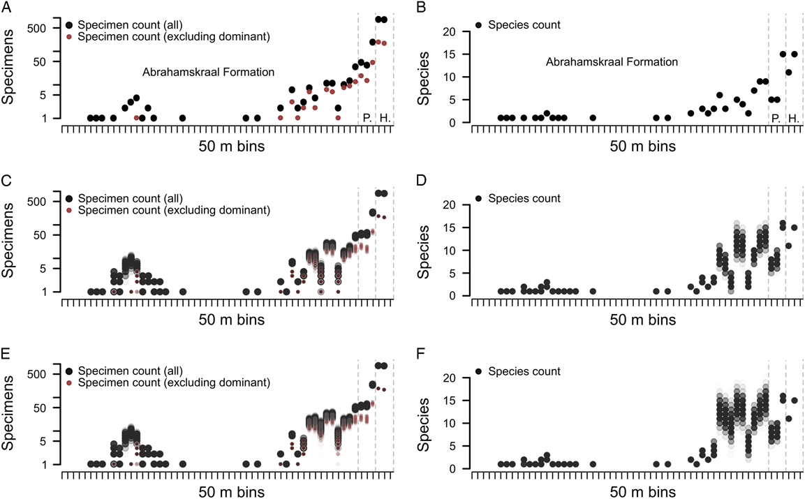
Our data set provides insights into sampling of fossil specimens through the mid–late Permian boundary interval of the Karoo Basin, indicating that few specimens have been collected from the lowermost 2000 m of the succession (Fig. 3). This lower portion of the succession has yielded important early therapsid specimens of the Eodicynodon AZ (Rubidge Reference Rubidge1995a; Rubidge and Hopson Reference Rubidge and Hopson1996). However, these are few in number, and individual 50 m stratigraphic bins have yielded generally fewer than 10 specimens. Furthermore, these specimens have been collected predominantly from an interval of approximately 450 m (nine stratigraphic bins in our analysis). A prominent gap exceeding 1000 m (20 stratigraphic intervals), from which only a handful of specimens has been recovered, separates this richer portion of the Eodicynodon AZ from the upper 600 m of the Abrahamskraal Formation (upper Tapinocephalus AZ, Capitanian). Fifty meter intervals in this latter portion of the succession have each yielded up to 30 specimens, which marks the beginning of continuous and well-sampled deposits extending into the late Permian. Because the lower deposits are not sufficiently rich or sampled continuously enough to provide information about species richness, extinction, or origination, our analyses focus on the upper portion of the succession.
Raw specimen (A, C, E) and species (B, D, F) counts for each 50 m stratigraphic bin in the Abrahamskraal Formation and lower Teekloof Formation at three levels of stratigraphic precision: using only specimens constrained to occur in a single bin (A, B), one of two bins (C, D), and one of three bins (E, F). Specimen counts increase from the upper Abrahamskraal Formation into the Poortjie and Hoedemaker Members of the Teekloof Formation, but species counts are universally lower in the lower two bins of the Poortjie Member than either before or after. Stratigraphy labeled in A and B only. P., Poortjie Member; H., Hoedemaker Member.

Specimen occurrence densities are greater still in the uppermost 50 m of the Abrahamskraal Formation and equivalent thicknesses of the lower Teekloof Formation (>45 specimens per interval). Despite this increase in counts of sampled specimens, species counts are typically similar to or lower than those of the preceding 450 m of the upper Abrahamskraal Formation (Fig. 3). Two alternative possibilities could explain why the observed increase in numbers of specimens sampled through the upper part of the succession does not result in an increase in species counted: (1) sampling of the preceding parts of the Abrahamskraal Formation, although less intensive, was already sufficient to recover most or all species that existed, so increasing the intensity of sampling does not increase the count of observed species; or (2) species richness was actually lower at the top of the Abrahamskraal Formation and in the Teekloof Formation, so much greater sampling intensity yields only species counts similar to those from the preceding intervals. These alternatives are tested below using equal-coverage subsampling (SQS). A decrease in the evenness of that assemblage, and particularly an increase in the relative abundance of the dominant taxon (Diictodon), could not explain this pattern: fewer taxa are counted in the first two bins of the Teekloof Formation even when the dominant taxon is excluded, even though (nondominant) specimen counts in these bins are similar to those of the upper 50 m of the Abrahamskraal Formation. This occurs because a large proportion of the increase in specimen counts is due to an increase in the abundance of the most common taxon, the dicynodont Diictodon (Figs. 3 and 4A). In fact, the relative abundance of Diictodon in the uppermost 50 m of the Abrahamskraal Formation is around 40%. This is more than twice the abundance of the preceding stratigraphic bin (100–50 m below the top of the Abrahamskraal Formation), and specimen counts from the uppermost 50 m of the Abrahamskraal Formation are similar to those in lower intervals when Diictodon is excluded (Fig. 3).
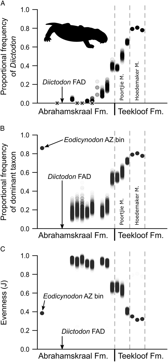
Dominance in the taxon abundance–frequency distribution in the Karoo Basin. A, Relative abundance of Diictodon from its first appearance datum (FAD) between 550 and 500 m below the top of the Abrahamskraal Formation in the northwest quadrant of the basin (the second appearance being 450–400 m below the top of the Abrahamskraal Formation). This was calculated conservatively by including only specimens identified definitively as Diictodon as a proportion of all specimens other than those identified as “Diictodon?,” “Diictodon??,” “pylaecephalid cf. Diictodon,” “pylaecephalid indet.,” “dicyndont_indet.,” or “dicynodont indet.” B, Relative abundance of the dominant taxon, regardless of identify, based on counts only of taxonomically diagnosable specimens. C, Evenness of the assemblage represented by Pielou’s J; note that this shows the inverse pattern to A and B. Only occurrences spanning 3 stratigraphic intervals of uncertainty, or fewer, were used in this figure, and these were randomly assigned to the stratigraphic bins from which they may have been collected over 1000 iterations. Proportions are only reported for stratigraphic intervals in which at least 10 specimens are present; intervals yielding 0 specimens of Diictodon are marked by gray crossed disks in A.

When quantifying evenness and dominance, we were concerned that the onset of the increase in the abundance of Diictodon might be artifactual in the Abrahamskraal Formation, where it overlaps with the range of dinocephalians and basal pareiasaurs. This is because Diictodon is readily recognizable from unprepared specimens (mostly skulls), whereas dinocephalians and pareiasaurs are difficult to identify even with good material; in most cases, dinocephalian finds consist of fragmentary skeletons dominated by postcranial elements that cannot be identified beyond the family level. Both dinocephalians and pareiasaurs also suffer from problematic taxonomy, exacerbating the problem. Consequently, it is possible that at least some, if not most, dinocephalian and/or pareiasaur genera may have survived later and at higher relative abundances than is reflected by our database and stratigraphic chart, thereby exaggerating the dominance of Diictodon (Fig. 1).
To control for this, we calculated the proportion of specimens in each interval belonging to Diictodon, counting even generically/specifically indeterminate occurrences of dinocephalians and other non-dicynodont tetrapods, which allowed far more specimens (representing genuine individuals of unknown genus) to be included. The relative abundance of Diictodon could thus be compared more fairly across the bins in which it occurs. This approach (not shown) suggests that “diagnosability” is unlikely to explain the increased abundance of Diictodon near the top of the Abrahamskraal Formation, because lower intervals of the Abrahamskraal Formation also contain abundant indeterminate tetrapods and should be affected in an identical way by this possible bias.
To examine variation in dominance or evenness, regardless of the identity of the dominant taxon, it is necessary to use only the occurrences of specimens that are diagnostic to a particular taxon. When this is done, most bins of the Abrahamskraal Formation, excluding bins containing fewer than 10 specimens, exhibit low dominance (the most abundant taxon has a relative abundance of 20%) and high evenness (Fig. 4B,C; Pielou’s J). The increases in Diictodon abundance described above are associated with large reductions in evenness and an increase in relative abundance of the dominant taxon to 60%. This shows that the evenness of the species abundance–frequency distribution is lower (i.e., more uneven) at the top of the Abrahamskraal Formation and in the Teekloof Formation than it is farther down in the stratigraphy, and this occurs specifically because of a stepwise increase in the dominance of Diictodon.
The proportional abundance of Diictodon continues to increase through the Poortjie Member of the Teekloof Formation (Pristerognathus AZ), reaching an acme in the Hoedemaker Member (Tropidostoma AZ); in this unit, around 80% of specimens belong to Diictodon, when a conservative calculation is used (Fig. 4A). The overall pattern is one in which Diictodon occurred at low proportional frequencies for 400–500 m (~3 Myr, based on an age of ca. 264 Ma for the mid-Abrahamskraal Formation and of 260.3 Ma for the top; Lanci et al. Reference Lanci, Tohver, Wilson and Flint2013; Day et al. Reference Day, Ramezani, Bowring, Sadler, Erwin, Abdala and Rubidge2015b) following its first occurrence, but subsequently underwent stepwise and cumulative increases in proportional abundance from the uppermost 50 m of the Abrahamskraal Formation onward.
No bins of the Eodicynodon AZ, in the lower part of the study interval, contain enough specimens to make confident estimates of dominance (arbitrarily designated as >10 specimens here). However, the combined data for 250–950 m from the bottom of our section contain in total 36 specimens, of which 31 belong to Eodicynodon, indicating a highly uneven abundance–frequency distribution here too.
Subsampled Species Richness
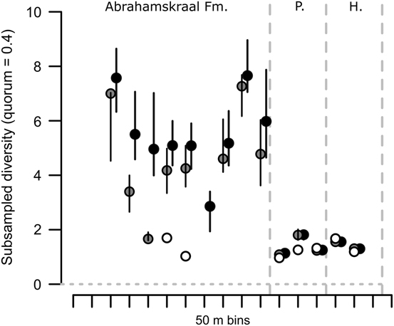
Subsampled species richness through the uppermost 450 m of the Abrahamskraal Formation is relatively high compared with that in the Teekloof Formation. This is found consistently at multiple quorum levels (q=0.4 is reported in Fig. 5) when occurrences with stratigraphic precision of two or three bins are used. When only strictly constrained stratigraphic occurrences are considered (one bin of stratigraphic precision), many fewer intervals have sufficiently high coverage to subsample effectively. Results therefore become uninformative. In fact, in this case, richness within the lower Abrahamskraal Formation can be estimated for a few intervals, which apparently have similar richness to the better-sampled boundary interval. This result is, however, based on a relatively small amount of data. We therefore favor the results of analysis using greater numbers of specimen occurrences with less precise stratigraphic data. It is unlikely that this introduces aliasing (= time-averaging) bias, because species turnover through the uppermost 500 m of the Abrahamskraal Formation is remarkably low (described below).
Mean subsampled species richness for stratigraphic bins using specimens constrained to one bin (white circles) and specimens constrained to two (gray circles) or three (black circles) bins and randomly assigned to one of them. Results are from all 1000 iterations of random assignment, and whiskers indicate interquartile ranges of the results from these iterations. Few bins contained sufficient occurrences to be subsampled when using only the best constrained occurrences (white circles). P., Poortjie Member; H., Hoedemaker Member.

Extinction and Origination Rates
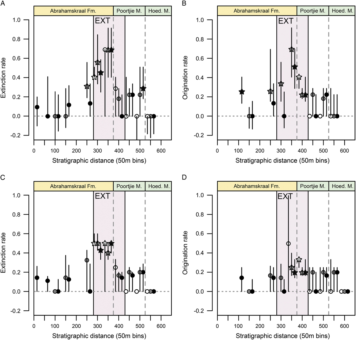
GF estimates of extinction rates are consistently found in all our analyses as being elevated to around 0.5 interval−1 in the penultimate 50 m of the Abrahamskraal Formation and to around 0.75 interval−1 in the uppermost 50 m of the Abrahamskraal Formation (Fig. 6A). Modified GF estimates of extinction proportion are similar, around 0.5 interval−1 for the final two bins (= top 100 m) of the Abrahamskraal Formation (Fig. 6C). Other stratigraphic intervals have distributions of estimated extinction rates whose interquartile ranges include zero, and median estimated extinction rates are typically positive (both methods). The lower interval of the Hoedemaker Member is the highest stratigraphic interval for which we were able to estimate extinction rates (using data from the preceding and two following stratigraphic intervals: the middle and upper portions of the Hoedemaker Member) and has a median estimated extinction rate of zero across all our analyses, except when only precisely dated specimen occurrences are used.
GF estimates of extinction (A) and origination (B) rates, and modified GF estimates of extinction (C) and origination (D) proportions for three levels of stratigraphic precision. White symbols indicate analysis using only occurrences that are assigned with certainty to a single 50 m stratigraphic interval; gray symbols show the results of analyses using occurrences with up to 2 bins of uncertainty; black symbols show the results of analyses using occurrences with up to 3 bins of uncertainty. Stars indicate rates for which the interquartile range did not include 0. Whiskers show standard interquartile ranges of results recovered from 1000 iterations, in which occurrences were randomly assigned to a single 50 m stratigraphic bin within the range of their uncertainty. Per-bin occurrence counts were standardized using classical rarefaction before rate estimation. Box marked “EXT” shows interval associated with the Capitanian mass extinction. Hoede M., Hoedemaker Member.

Dinocephalians make a large contribution to the occurrence of extinctions in the upper portions of the Abrahamskraal Formation (i.e., dinocephalian species disproportionately become extinct). The presence of rare dinocephalians in the lower portion of the Poortjie Member (Fig. 1; Day et al. Reference Day, Güven, Abdala, Jirah, Rubidge and Almond2015a) is therefore curious, and raises questions about whether a small number of dinocephalian lineages survived a short time after the extinction event. Alternatively, an abrupt extinction of all dinocephalians during a brief interval of time equivalent to the upper Abrahamskraal Formation could still occur if the base of the Poortjie was slightly diachronous. In fact, radiometric and biostratigraphic data suggest that the base of the Poortjie is among the most isochronous timelines within the lower Beaufort Group (Rubidge et al. Reference Rubidge, Erwin, Ramezani, Bowring and de Klerk2013; Day et al. Reference Day, Ramezani, Bowring, Sadler, Erwin, Abdala and Rubidge2015b). We therefore suggest that the evidence is consistent with the survival of at least one dinocephalian species beyond the main extinction pulse in the upper Abrahamskraal Formation. This is comparable to observed therapsid turnover during the end-Permian extinction event, in which several therapsid groups survive as “dead clades walking” (Jablonski Reference Jablonski2002) following the main extinction pulse but disappear from the record shortly thereafter (e.g., akidnognathid therocephalians; Smith and Botha Reference Smith and Botha2005).
Origination rates show a background pattern of generally low median values, with interquartile ranges that include zero. Median origination rate estimates are high in the upper 50 m of the Abrahamskraal Formation, and elevated (although less so) in the lower 50 m of the overlying Poortjie Member based on the GF method (Fig. 6B). They are not elevated according to the modified GF method, although their confidence intervals exclude zero, suggesting a weak pulse of origination compared with background (Fig. 6D). This latter result is more consistent with patterns of subsampled richness, which is low from the start of the Poortjie Member, in turn suggesting that postextinction origination rates were not sufficient to recover substantive standing diversity (Fig. 5).
Discussion
The boundary between the Abrahamskraal Formation and Poortjie Member of the Teekloof Formation is a near-isochronous horizon in the Karoo Basin, possibly related to basin-wide tectonic influence (see Paiva Reference Paiva2016). Using robust estimates of patterns of species richness, extinction rates, and origination rates, we find evidence of strongly elevated extinction rates in the upper 100 m of the Abrahamskraal Formation. This coincides with a reduction of species richness that persisted through the Poortjie and Hoedemaker Members of the Teekloof Formation. Origination rates were only weakly elevated in the upper Abrahamskraal Formation and lower Poortjie Member. Although the GF method suggests that origination rates reached levels similar to extinction rates in the last interval of the Abrahamskraal Formation (Fig. 6A,B), this was not obtained using the modified GF method (and is the largest discrepancy between these two modes of analysis). Furthermore, even if the GF result is correct, origination rates are based on the number of taxa crossing the upper boundary of the interval, whereas extinction rates are based on the proportion of taxa crossing the lower boundary. Because more taxa cross the lower boundary, as a result of high extinction within the interval, the number of lineages crossing into the following bin is much lower. Thus, even relatively few absolute originations would appear as an apparently high origination rate. Our results demonstrate that the late Capitanian–aged upper Tapinocephalus AZ of the Main Karoo Basin represents a high-diversity tetrapod assemblage, whereas the assemblages of the Pristerognathus AZ and early Wuchiapingian (early Lopingian) lower Tropidostoma AZ had low richness.
The finding of low species richness in the early late Permian of the Karoo Basin is consistent with a previous study that used rarefaction to estimate species richness at coarse stratigraphic resolution (Irmis and Whiteside Reference Irmis and Whiteside2011). Using high-resolution stratigraphic data divided into approximately 50 m stratigraphic intervals, we find consistent estimates of species richness in multiple successive bins on intermediate timescales, providing greater confidence in this conclusion. By accounting for sampling differences, this demonstrates that the Pristerognathus AZ and at least the lower part of the Tropidostoma AZ document a taxonomically impoverished, postextinction tetrapod assemblage spanning approximately 2 Myr between the late Capitanian and early Wuchiapingian (Rubidge et al. Reference Rubidge, Erwin, Ramezani, Bowring and de Klerk2013; Day et al. Reference Day, Ramezani, Bowring, Sadler, Erwin, Abdala and Rubidge2015b). Although the Tapinocephalus AZ has yielded more fossils from a greater number of localities, these are spread over a much greater stratigraphic thickness, and the precision with which fossils can be placed within it is much lower. Fossil occurrences per unit thickness in the Tapinocephalus AZ are also low (Fig. 3). Nevertheless, many genera have been sampled in the upper few hundred meters of the Abrahamskraal Formation. Conversely, the Pristerognathus AZ has produced a relatively large number of fossils given its lesser thickness, and fossil occurrences in that biozone have better stratigraphic precision. We cannot, therefore, attribute the lower subsampled diversity of the Pristerognathus AZ to lower sampling, and this is especially true given that we use equal-coverage subsampling to estimate richness while accounting for differences in sample coverage throughout the stratigraphy.
Previous work has documented low evenness in the abundance frequency distribution of tetrapod species in the Tropidostoma AZ (Irmis and Whiteside Reference Irmis and Whiteside2011). Low evenness (= high dominance) is often associated with ecosystem instability and is a characteristic of postextinction “recovery” faunas. Our high-resolution stratigraphic data indicate that the transition from high to low evenness results from the increase in abundance of the dicynodont Diictodon, which began below the upper 50 m of the Abrahamskraal Formation and, therefore, before the peak of Capitanian extinction rates. Although the increasing dominance of Diictodon leads to low evenness in genus frequency distributions in the uppermost bins of the Abrahamskraal Formation, the magnitude of this unevenness continues to grow into the succeeding Poortjie and Hoedemaker Members of the Teekloof Formation. We therefore suggest that the increasingly exceptional dominance of Diictodon during the latest Capitanian and early Wuchiapingian represents opportunistic expansion in an unstable ecosystem, beginning before the acme of species extinctions and continuing after them.
Together with the observation of low levels of dinocephalian survival into the lower 50 m of the Poortjie Member, this suggests that the Capitanian extinction event among tetrapods in the Karoo Basin was a dynamic process occurring over an interval of more than 100 m of stratigraphy. Estimates of depositional rates for the upper Abrahamskraal Formation exist from the eastern Karoo Basin, based on rock thickness between dated tuff horizons (Day et al. Reference Day, Ramezani, Bowring, Sadler, Erwin, Abdala and Rubidge2015b: Supplementary Information 1.C). These suggest that about 130–150 Kyr is represented per 50 m. Alternatively, if we assume a constant rate of deposition between the top of the Abrahamskraal Formation (260.3 Ma; Day et al. Reference Day, Ramezani, Bowring, Sadler, Erwin, Abdala and Rubidge2015b) and the mid-Abrahamskraal Formation (~264 Ma; Lanci et al. Reference Lanci, Tohver, Wilson and Flint2013; but see Day and Rubidge Reference Day and Rubidge2014), then 50 m of rock would represent 138–250 Kyr. Dates from a single locality in the western margin of the basin alone suggest approximately 330 Kyr per 50 m (Lanci et al. Reference Lanci, Tohver, Wilson and Flint2013). Thus, although depositional rates were no doubt variable and these estimates need to be treated very tentatively, we propose that the extinction event took place over 0.3–0.6 Myr.
Comparison with Previous Sampling-corrected Diversity Estimates for Tetrapods
Our results contrast with several previous studies of tetrapod taxonomic richness during the mid- to late Permian. Reasons for this include differences in methodologies used to estimate (or count) species richness, whether and how those methods attempt to standardize variation in sample size/coverage, the quality of the data sets used, and the geographic and temporal scale at which they were conducted. For instance, in a study of global paleodiversity patterns among Permian tetrapods, Benton et al. (Reference Benton, Ruta, Dunhill and Sakamoto2013) found that a number of diversity crises appear to have occurred in the late Paleozoic but failed to find any crisis in the Capitanian. Instead, they identified a diversity decline in the Wordian (early Guadalupian, 5–8.5 Myr before the event documented here) and another in the early Wuchiapingian (1–6 Myr after the event documented here). To this latter event they attributed an 81% loss of genera (92 out of 113), but this appears to be based erroneously on ratios of originations rather than extinctions (Benton et al. Reference Benton, Ruta, Dunhill and Sakamoto2013: Supplementary Table S1). When this is corrected, the early Wuchiapingian has an ~58% proportional extinction (as a proportion of total diversity within the substage), and extinction rate peaks stand out in the late Kungurian (i.e., early to mid-Permian transition; 91%), lower (early) Capitanian (77%), and Changhsingian (i.e., Permian/Triassic transition; 89%), much more in line with expectations. Furthermore, the extinction peak in their “lower Capitanian” corresponded to the loss of diversity between the Tapinocephalus AZ and the Pristerognathus/Tropidostoma AZs, which radiometric ages published subsequently have shown to actually be within the late Capitanian (Day et al. Reference Day, Ramezani, Bowring, Sadler, Erwin, Abdala and Rubidge2015b). When per-taxon extinction rates are calculated for the same data set, but taking into account stage duration, the same peaks remain. Benton et al. (Reference Benton, Ruta, Dunhill and Sakamoto2013) did not generate sampling-corrected global diversity estimates due to the difficulty of accounting for the plethora of factors that bias the fossil record on a global scale.
Regional studies suffer from fewer distinct types of bias than global studies. In particular, regional-scale studies are not affected by temporal fluctuations in the number of sampled regions (i.e., areas of the Earth that have yielded fossils) that occurs in “global” studies. Because sampling a new region is likely to produce greater numbers of species, this is arguably the largest bias on apparently “global” paleodiversity assessments (e.g., Alroy Reference Alroy2010b). For instance, Benson et al. (Reference Benson, Butler, Alroy, Mannion, Carrano and Lloyd2016) showed that the paleogeographic extent of global fossil localities explained at least 60% of the variance in species and genus counts for Mesozoic tetrapods. On the other hand, while the Main Karoo Basin is a fine natural laboratory, it is not necessarily representative of global patterns of diversity change. Regional studies in other basins, particularly at different latitudes, may therefore differ in their results, but by limiting a study to a single region, as done here, we provide one solution to the problem of “geographic sensitivity” experienced at a global level (see Close et al. [Reference Close, Benson, Upchurch and Butler2017] for a broader method).
Studies of the Main Karoo Basin and the fore-Ural region of the Russian platform have attempted to standardize for sample availability using residual diversity estimates, derived from differences between modeled diversity assuming complete dependence on a sampling proxy and observed diversity (Fröbisch Reference Fröbisch2013, Reference Fröbisch2014). Such proxies have included the number of localities, number of specimens, and, in the case of the Karoo, total outcrop area. This approach found positive residuals for the Pristerognathus AZ, suggesting higher species richness than could be explained by the sampling proxy (outcrop area; Fröbisch Reference Fröbisch2013). In other words, it provided little support for a Capitanian extinction in terms of taxic diversity loss, because richness appeared to be higher after this event than before it.
Fröbisch (Reference Fröbisch2013) primarily used outcrop area to correct face-value taxon counts, but this and other “rock amount” measurements only influence sampling intensity indirectly, by providing rock from which to sample fossils. Fröbisch (Reference Fröbisch2013, Reference Fröbisch2014) also considered the number of specimens actually collected as a sampling proxy; we consider this to be preferable, given that it more accurately reflects the high intensity of collecting in the Pristerognathus AZ (e.g., Fig. 3). When species counts were corrected for counts of specimens sampled, the residual diversity was negative for synapsids, more similar to our findings here (Fröbisch Reference Fröbisch2013: Supplementary Fig. S2), although the same was not true of other tetrapods (Fröbisch Reference Fröbisch2013: Supplementary Figs. S3–S5). The positive diversity residuals for non-synapsid tetrapods found by Fröbisch (Reference Fröbisch2013) may be partly due to the presence in the Pristerognathus AZ (in his data set) of the pareiasaurs Bradysaurus and Embrithosaurus, the biarmosuchian Hipposaurus, and the rhinesuchid temnospondyl Rhinesuchoides, taxa that we do not consider to occur in that assemblage zone. Inspection of our specimen counts suggests that face-value species counts in the Pristerognathus AZ are in fact low in comparison to the number of specimens sampled (Fig. 3), consistent with our relatively low subsampled richness estimates.
An alternative method for estimating global richness is a form of range-through diversity estimate that uses information from phylogeny in addition to taxon ranges, known as phylogenetic diversity estimation (Norell Reference Norell1992; Smith Reference Smith1994). So far this has been applied to data sets for parareptiles (including pareiasaurs) and anomodonts (including dicynodonts) through the mid–late Permian (Ruta et al. Reference Ruta, Cisneros, Liebrecht, Tsuji and Müller2011, Reference Ruta, Angielczyk, Fröbisch and Benton2013), amniotes from the Carboniferous to the Triassic (Brocklehurst et al. Reference Brocklehurst, Ruta, Müller and Fröbisch2015), and for temnospondyls at the family level (Ruta and Benton Reference Ruta and Benton2008); these studies have indicated an increase in richness above the Capitanian, in direct contrast to our findings. However, their conclusions are partly attributable to the coarse time resolution of these studies: for instance, Ruta et al. (Reference Ruta, Angielczyk, Fröbisch and Benton2013) observed an increase in richness between the Capitanian and Wuchiapingian but used the sum of ranges within these extended time intervals, which both exceed 5 Myr in duration (i.e., approximately one-tenth of the temporal precision of our analyses).
Overall, our finding of an elevated extinction rate for the tetrapod community in the upper 100 m of the Abrahamskraal Formation is consistent with the stratigraphic ranges of taxa (Fig. 1) and with counts of last appearances derived from constrained optimization of range-end events that was performed on an older (smaller) version of this same data set (Day et al. Reference Day, Ramezani, Bowring, Sadler, Erwin, Abdala and Rubidge2015b). This latter used minimum stratigraphic range lengths alone and was not so well tied to the lithostratigraphy, with some uncertainty remaining over the exact position of the extinction peak. The reason for this is because the CONOP algorithm considers only the relative positions of events, regardless of lithostratigraphic provenance, so that such contacts can only be projected onto the optimal sequences of first- and last-appearance events when considered as events themselves; their position relative to the sequence of last appearances is therefore variable. By using stratigraphic bins measured from a relatively isochronous lithostratigraphic horizon, that is, the base of the Poortjie Member, our analyses assign this contact an a priori fixed position, and so the distance from the contact can be more accurately observed.
Time Standardization
The comparison between our results and the studies above suggest that the temporal resolution of data sets used in the determination of richness and of turnover rates can be influential. Shen and Shi (Reference Shen and Shi2002) were aware that long time bins (i.e., for the Lopingian) may have masked diversity loss in brachiopods, while this possibility was also recognized more generally by Bambach et al. (Reference Bambach, Knoll and Wang2004). This poses a problem, because analytically adjusting species richness estimates, turnover rates, or other metrics using information on time-bin duration will not be sufficient to correct the findings from databases with coarse stratigraphic resolution, and in fact can introduce substantial error. The reason is that if a rapid extinction event occurs in a long time bin, then its apparent severity will be diluted across the whole interval, though this is also dependent on the magnitude of background rates both absolutely and relative to the mass extinction. Conversely, if it occurs in a very short bin, then it will be divided by a lesser amount of time and appear greater. An extinction event of the same magnitude would thus appear much less severe if it occurred in a 5.5 Myr bin than if it occurred in a 1 Myr bin, even if background rates were constant. This would make comparisons of the mid-Permian (Capitanian=5.5 Myr; Wuchiapingian=5 Myr) and Permo-Triassic (Changhsingian=2.2 Myr; Induan=0.7 Myr) mass extinctions unfair. Time-standardized rates may be especially problematic in the Karoo, because the Tapinocephalus AZ is mostly sampled from the upper part of the zone; time corrections assuming it spans the length of the Capitanian may thus underestimate extinction rates.
A rate metric that is better able to quantify mass extinction intensity at this stage resolution involves identifying mass extinctions a priori and then accounting for background extinction as calculated from intervals in which such events do not occur (Stanley Reference Stanley2016). Of course, this requires recognition of these events in the first place, which may only be apparent at the regional level. Indeed, our results show that at high stratigraphic resolution, a distinct increase in extinction rates and corresponding drop in richness is apparent in the late Capitanian, which eluded previous studies at coarser, standardized timescales. Furthermore, evolutionary rates appear to be multidimensional, so they are unlikely to be reliably described by single metrics employed at different temporal scales. This remains a problem when trying to understand “background” extinction rates and elevated, mass extinction rates simultaneously. The best approach could be to combine low-resolution trends with high-resolution studies at focal intervals while isolating rate anomalies and, ultimately, to adjust long-term trend lines accordingly.
Conclusions
Global data sets may be unable to identify rapid turnover or extinction events, especially when they occur in longer time bins. This may be true even when such events had a profound effect on an ecosystem, particularly if the extinction occurs only at lower taxonomic levels. When such cases arise, regional stratigraphic studies must be relied on to correctly interpret the fossil record. We applied probabilistic methods to a high-resolution fossil data set to constrain the timing of evolutionary events among terrestrial tetrapods in the mid/late Permian boundary interval of the Main Karoo Basin. This differs from previous approaches that used coarsely resolved occurrence data and taxon counts (rather than subsampled richness estimates) or that considered first and last occurrences to represent literal originations and extinctions.
Sampling across most of the Tapinocephalus and Eodicynodon AZs is insufficient to infer patterns of diversification, but sampling is generally good over the upper Tapinocephalus and Pristerognathus AZs when using specimen occurrences and when the thickness of the zones is taken into account. These assemblage zones document the mid–late Permian transition in South Africa, including turnover associated with the Capitanian mass extinction. The peak in the extinction rate occurs predominantly at the top of the Tapinocephalus AZ (uppermost Abrahamskraal Formation), despite the occurrence of at least one dinocephalian genus in the lower Poortjie, which likely represents a “dead clade walking” (sensu Jablonski Reference Jablonski2002).
An increase in the unevenness of taxon-abundance frequency distributions is also associated with the Capitanian extinction event. This is caused by the increasing dominance of the dicynodont Diictodon, a robust finding even when accounting for taphonomic biases. A large increase in Diictodon abundance, and the resulting decrease in evenness, presages the peak of extinction rates by one 50 meter bin; it was therefore not caused directly by the disappearance of other species, although it may reflect a reaction to ecosystem perturbation in advance of the Capitanian extinction peak.
Our results are broadly congruent with those reported by Day et al. (Reference Day, Ramezani, Bowring, Sadler, Erwin, Abdala and Rubidge2015b) using constrained optimization of range-end events (75–80% diversity loss), but go further, in that (1) they more precisely constrain the lithostratigraphic position of the extinctions and (2) they show that the postextinction Pristerognathus AZ represents an interval of low diversity compared with the Tapinocephalus AZ, which cannot be explained by poor sampling. This relatively low richness continues into the lower part of the overlying, late Permian (early Wuchiapingian) Tropidostoma AZ and suggests that recovery of species richness in the Main Karoo Basin was delayed for several million years after the Capitanian extinction event. Although the Pristerognathus AZ does exhibit elevated origination rates, these were not sufficient to balance the loss of richness resulting from the extinction event. At larger scales, the loss of biodiversity in the Main Karoo Basin may have been greater than in other parts of Gondwana, perhaps because of its higher latitude, but data on regions outside the basin remain inadequate to examine at the resolution used here. Nevertheless, in key areas such as the Main Karoo Basin, the Capitanian extinction event precipitated a long period of low species richness that paved the way for the late Permian tetrapod radiation.
Acknowledgments
The authors wish to thank the NRF/DST Centre of Excellence in Palaeosciences (CoE-Pal), the African Origins Platform of the National Research Foundation of South Africa (NRF), and the Palaeontological Scientific Trust (PAST) and its Scatterlings of Africa programs for generous financial support. C.F.K.’s research was supported by a grant from the Deutsche Forschungsgemeinschaft (KA 4133/1-1).
Supplementary material
Data available from the Dryad Digital Repository: https://doi.org/10.5061/dryad.683br42