





1 Introduction
In the field of mathematical modelling of diffusive processes in physical and biological phenomena, some of the most technically challenging and interesting are those that involve degenerate diffusion . A canonical example of degenerate diffusion is the porous medium equation [Reference Aronson2, Reference Vázquez28]:

where m is a constant exponent. In this equation, the diffusivity
$v^m$
 vanishes at points where
$v=0$
 . As long as
$m>0$
 , given an initial condition that is exactly zero to the right of a point
$x^*_0$
 , for example, a piecewise step function

solutions to (1.1) exist that feature a singular point
$x^*(t)$
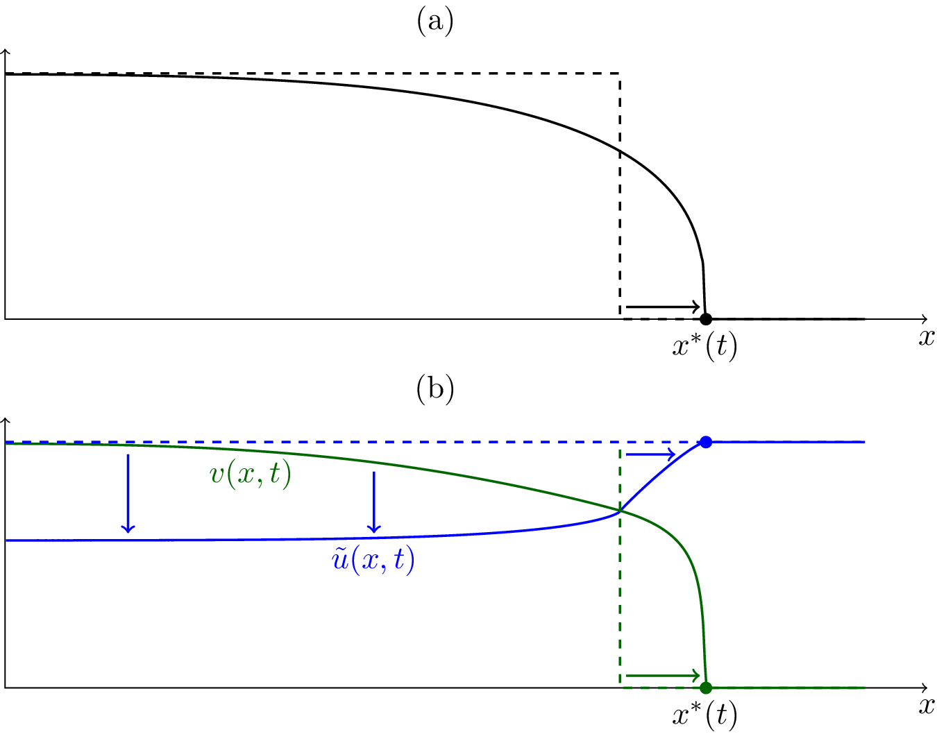
 ; at such a point, the solution (and therefore the diffusivity) vanishes (see Figure 1(a)). In the porous media literature, such a point is called an interface or free boundary. Explicit solutions exist that exhibit such an interface, for example, the Barenblatt–Pattle similarity solution [Reference Barenblatt3, Reference Pattle23]; an advantage of an initial step function (1.2) is that the resulting solution will also exhibit self-similarity. Any such solution must be defined in a weak sense, as the derivatives of v in (1.1) will typically not exist at the interface itself.


Adding a logistic reaction term to (1.1) results in the porous Fisher equation, a degenerate-diffusion version of the classical Fisher–Kolmogorov–Petrovsky–Piskunov (Fisher–KPP) problem, which has been of significant interest in mathematical biology [Reference Aronson1, Reference de Pablo and Sánchez12, Reference Newman22, Reference Sanchez-Garduno and Maini24]. The degenerate nature of the problem near an interface is unchanged by the inclusion of the reaction term. In this instance, most interest has been in the existence of travelling wave solutions; the porous Fisher equation has a unique travelling wave solution (in contrast to the continuum of travelling waves of the classical Fisher–KPP problem) and that solution exhibits an interface.
More recently, degenerate reaction-diffusion systems that feature multiple species have been considered in the context of biological cell invasion and interaction. These models may be complicated by cross-diffusivity, in which the population of one species affects the diffusivity of another. One such class of two-species models features a nonmotile resident cell population
$\tilde u$
 and a diffusive invading cell population v, which are coupled by
$\tilde u$
 inhibiting the spread of v, while at the same time, v degrades the local population of
$\tilde u$
 , and thus indirectly increases its own diffusivity. Nondimensionally, these models may take the form


An example of previously studied systems of this form is the approximation [Reference Gallay and Mascia17, Reference Mascia, Moschetta and Simeoni21] of the Gatenby–Gawlinski model of acid-mediated tumour growth [Reference Gatenby and Gawlinski18], for which F and G are logistic terms in
$\tilde u$
 and v, respectively. Other similar examples are those considered in [Reference Colson, Sánchez-Garduño, Byrne, Maini and Lorenzi8], which are similar but neglect the recovery of the resident population
$\tilde u$
 (
$F\equiv 0$
 ) and the model considered in [Reference Browning, Haridas and Simpson5, Reference Chen and Dallaston7, Reference El-Hachem, McCue and Simpson15], which similarly neglects growth of
$\tilde u$
 but includes the effects of inhibition of
$\tilde u$
 on the carrying capacity of v, in addition to its diffusivity.
Models such as (1.3) are simple cases of general Keller–Segel-type systems that may include both nonlinear, signal-dependent motility (diffusivity) and taxis (that is, flux proportional to gradients of the other species) [Reference Fu, Tang, Liu, Huang, Hwa and Lenz16, Reference Jin, Kim and Wang20, Reference Wang and Wang29]. Generally, such systems are qualitatively different to (1.3) (and more regular) as both species diffuse; in such models,
$\tilde u$
 takes the role of a signalling agent rather than a resident population. However, systems that include taxis-like “volume-filling” effects in the flux, but a nondiffusive resident population as in (1.3), have been recently considered in the context of continuum limits of discrete agent-based cell models [Reference Crossley, Maini, Lorenzi and Baker9, Reference Crossley, Pietschmann and Schmidtchen10, Reference Simpson, Murphy, McCue and Buenzli25].
The degeneracy of models of the form (1.3) arises when the resident cell population is at its capacity. An initial configuration that explores this degeneracy, and is also relevant from the perspective of modelling cell invasion, has the resident population initially at its capacity, with the invading population initially localized to a compactly supported region. An example, similar to (1.2), is thus

In analogy to the porous medium equation (1.1), a crucial question is whether there are (weak) solutions of this model that feature a propagating interface. In the context of (1.3), an interface is a point at which the resident population
$\tilde u$
 is at its carrying capacity while the invading population v is at zero. A schematic of this setup is shown in Figure 1(b).
The existence or otherwise of such an interface has not been conclusively settled by previous studies. On the one hand, there are a number of examples of numerical simulations of partial differential equations (PDEs) of the form (1.3) with initial conditions (1.4) that do appear to have a propagating interface, often evolving to travelling wave solutions (depending on the form of the reaction terms F and G) [Reference Colson, Sánchez-Garduño, Byrne, Maini and Lorenzi8, Reference El-Hachem, McCue and Simpson15, Reference Mascia, Moschetta and Simeoni21]. On the other hand, in [Reference Gallay and Mascia17], it was shown that a one-parameter family of travelling waves to their model must exhibit algebraic decay of V in front of the wave, rather than an interface at a finite location. The front of the wave becomes steeper in the limit where the speed of the wave is taken to zero. In addition, numerical estimates of the wave speed from PDE simulations made in [Reference Mascia, Moschetta and Simeoni21] indicated minor but nonnegligible dependence on the spatial resolution of the numerical scheme, raising concerns as to whether the results of the PDE simulations had in fact numerically converged.
In this article, we consider in depth an idealized version of systems of the form (1.3) that includes the coupled effects of degenerate cross-diffusion and degradation:

Here, we have defined the resident population deficit
$u = 1-\tilde u$
 , so that u may be considered the (time-and-space-dependent) diffusivity itself and
$u=0$
 represents the resident population at capacity. We are particularly interested in whether we can find solutions for which the diffusivity is initially zero and the invading population is compactly supported, such as in (1.4). However, an initially compactly supported v will (in stark contrast to the porous media equation (1.1)) prove to be problematic. We thus consider the initial condition

where the initial height in front of the discontinuity
$\epsilon \in (0,1)$
 . To examine the possibility of a solution with an interface, we will then focus on the limiting behaviour as this leading height,
$\epsilon $
 , becomes small.
Our main finding will be that the limit
$\epsilon \to 0$
 is singular. While for small
$\epsilon $
 , an apparent interface (a point at which v is small and the slope of v is large in
$\epsilon $
 ) will be present, the speed of propagation of this point vanishes and the slope of the profile becomes infinite, as
$\epsilon \to 0$
 . Our conclusion is thus that the system (1.5) does not support solutions that have a moving interface, in contrast to systems such as the porous medium equation (1.1). However, this limit turns out to be approached logarithmically slowly in
$\epsilon $
 (to be precise,
$O([\log (1/\epsilon )]^{-1/2})$
 ), which explains why numerical simulations of such models may appear to converge, as they have numerically regularized the problem at
$O(\epsilon )$
 , while observed quantities such as speeds of propagation superficially appear to be order one.
We start in Section 2 by showing an example numerical simulation of (1.5) and demonstrate how solutions for any given
$\epsilon> 0$
 can be found by solving a similarity solution rather than the full PDE. The numerical calculation of these similarity solutions shows a number of interesting properties, including the possibility of persistent nonexistence of spatial derivatives of u (and higher spatial derivatives of v) over time, as well as showing the first indication of logarithmically slow behaviour of solution parameters (such as the speed of propagation) in the
$\epsilon \to 0$
 limit. In Section 3, we perform a matched asymptotic analysis of the similarity solution for small
$\epsilon $
 , which confirms this logarithmic behaviour. We discuss the more general implications of these results and future extensions in Section 4.
2 Numerical solutions and self-similarity
To demonstrate the generic behaviour of the PDE system (1.5) with initial condition (1.6), we simulate the system numerically. This is performed on a finite domain
${0 < x < 5}$
 , with no-flux conditions on v at the ends (no boundary conditions are required for u as it has no spatial derivatives). The initial discontinuity is taken at the centre of the domain at
$x^*_0 = 2.5$
 . The PDE is discretized in space using a finite volume method implemented in MATLAB and advanced in time using MATLAB’s ode15s implicit time stepping algorithm. The details of this method are quite standard and very similar to those used in [Reference Chen and Dallaston7], so we do not go into further detail here.
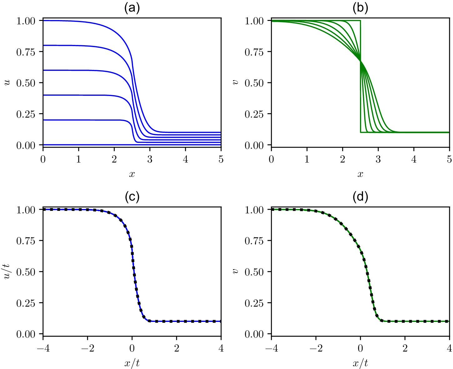
We show the results of such a simulation for
$\epsilon =0.1$
 in Figure 2(a,b) for u and v, respectively. Solution profiles are shown for equally spaced times from
$t=0$
 to
$t=1$
 . This solution demonstrates the coupled behaviour of the two variables, with u increasing more rapidly to the left of the initial discontinuity and v diffusing in both directions, although more rapidly to the left of the initial discontinuity and more slowly to the right. This behaviour is as expected given that u is the diffusivity of v.
Numerical solutions of the PDE system (1.5) for (a)
$u(x,t)$
 and (b)
$v(x,t)$
 , at evenly spaced times t from
$0$
 to
$1$
 . The initial condition is (1.6) for
$\epsilon = 0.1$
 . (c), (d) PDE simulations at the times plotted in panels (a,b) (except for the initial condition
$t=0$
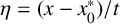
 ) scaled onto similarity variables
$\eta = (x-x^*_0)/t$
 ,
$f = u/t$
 ,
$g = v$
 , showing exact collapse to a similarity solution. Black dotted curves are the corresponding numerical solution of the ordinary differential equation (ODE) system (2.2).

2.1 Formulation of system for similarity solution
While the system can be simulated as above for any
$\epsilon $
 , a chief advantage of considering the simplified model (1.5) with initial condition (1.6) is that it permits a similarity solution. This similarity solution may be calculated numerically by solving a single boundary value problem with much greater precision than the original PDE, which will be particularly valuable when looking at small values of the height
$\epsilon $
 in front of the initial discontinuity. We also note that, while exact for the simplified model (1.5), this similarity solution also represents the early-time behaviour of more complex cross-diffusion models of the form (1.3) evolving from an initial condition (1.6), and so captures essential behaviour of this class of models as well (see Section 4 for further discussion).
To construct similarity solutions, we first define the similarity variable
$\eta $
 , and similarity profiles f and g by

The factors t in (2.1) result from requiring the terms in (1.5) to have the same dependence on t, while the scale of v cannot change as it must match to the fixed values behind and ahead of the initial discontinuity in the large
$\eta $
 limit. From (1.5), the profiles f and g then satisfy the ordinary differential equation (ODE) system

with far-field conditions consistent with the initial condition (1.6):

As
$t\to 0^+$
 , the profiles contract around the point
$x=x^*_0$
 ; thus, a similarity solution satisfying these conditions will approach the correct initial condition (1.6).
Looking closer at the far-field conditions (2.3), if we expand f and g close to a constant in each far-field
$|\eta |\to \infty $
 , we find that (2.2) supports the behaviour

for
$C_0$
 ,
$C_1$
 constants, and the Wentzel–Kramers–Brillouin (WKB) prefactor
$C_2$
 is a function of
$\eta $
 (whose exact form is unimportant). To satisfy the far-field conditions, we require
$C_0 = 1$
 for
${\eta \to -\infty }$
 and
$C_0 = \epsilon $
 for
$\eta \to \infty $
 , while the algebraically growing mode
$C_1$
 must be zero in both cases. The remaining WKB mode decays exponentially in each case. Thus, each far-field condition effectively applies two constraints on the system, resulting in four boundary conditions for the third-order system (2.2).
To find solutions then, an additional degree of freedom is required. This is provided by the fact that the system (2.2) is singular at the point at
$\eta = 0$
 . Expanding f and g near
$\eta =0$
 , we find that f may be nondifferentiable; in particular,

where
$a_0$
 ,
$a_1$
 ,
$a_2$
 are arbitrary, and all higher coefficients may be determined in terms of these three constants. For g to be differentiable across the singular point,
$a_0$
 and
$a_1$
 must take the same value on either side of
$\eta =0$
 . However,
$a_2$
 may take different values on either side, say

This extra degree of freedom allows us to satisfy both far-field conditions. A consequence of the singular point is that even for time greater than zero, u will be nondifferentiable at the point
$x_0$
 at which the initial discontinuity existed. The PDE system (1.5) permits this because there is no diffusion of u.
2.2 Numerical calculation of similarity solutions
We now describe the method of numerically calculating solutions of (2.2). To achieve high accuracy and observe the change in profiles as
$\epsilon $
 is varied, we use the numerical continuation package AUTO-07p [Reference Doedel, Champneys, Dercole, Fairgrieve, Kuznetsov, Oldeman, Paffenroth, Sandstede, Wang and Zhang13]. To obtain a solution with the appropriate boundary conditions (2.4), we will apply a homotopy continuation method, in which an initial trial solution is computed with explicit error terms in the boundary conditions, which are then each reduced to zero in turn via numerical continuation. This process has been applied to the computation of similarity solutions previously with much success [Reference Dallaston, Tseluiko, Zheng, Fontelos and Kalliadasis11, Reference Tseluiko, Baxter and Thiele27].
To correctly treat the singular point at
$\eta =0$
 , we formulate the system as two sets of ODEs, one starting at
$\eta = -\Delta \eta $
 , just to the left of the singular point and extending to
$\eta = -L$
 in the negative direction, and one starting from
$\Delta \eta $
 and extending to
${\eta = R}$
 in the positive direction. Here,
$\Delta \eta \ll 1$
 and
$R,L \gg 1$
 ; in our calculations, we take
${\Delta \eta = 10^{-4}}$
 ,
$R=8$
 , and
$L=5$
 ; the exponentially decaying term in (2.5) means that the far-field condition is approached rapidly in each direction, so L and R do not have to be very large. Defining the scaled flux variable
$h(\eta ) = u(\eta ) v'(\eta )$
 , we then have the system

where
$\pm $
 superscripts refer to the positive and negative
$\eta $
 -directions, respectively.
Close to the singular point, we use the expansion (2.5) as boundary conditions:

Here,
$a_0$
 ,
$a_1$
 and
$a_2^\pm $
 are parameters that will be varied to satisfy the far-field conditions. In the far field, we apply

Here,
$\mathcal E^{\pm }$
 represents error terms from the desired boundary conditions (2.3) (in which f and g are equal), while
$C_0^\pm $
 represents each far-field value. The aim of the homotopy continuation procedure will be to reduce each of
$\mathcal E^\pm $
 to zero, set
$C_0^- = 1$
 and
$C_0^+ = \epsilon $
 for any given
$\epsilon $
 .
We proceed as follows. We start with the exact linear solution to (2.2),
$f = \eta /2$
 ,
${g = 1}$
 , with domain size parameters
$R = L = 1$
 (the parameter
$\Delta \eta = 10^{-4}$
 is held constant throughout the continuation procedure). This initial solution then satisfies the imposed boundary conditions, given the parameter values:

We then apply numerical continuation, first reducing the left-hand error
$\mathcal E^-$
 to zero and the left-hand value
$C_0^-$
 to one, while letting
$a_0, a_2^-$
 and
$\mathcal E^+$
 vary. We then reduce the right-hand error
$\mathcal E^+$
 to zero and
$C_0^+$
 to
$\epsilon =0.1$
 , letting each of
$a_0, a_1, a_2^\pm $
 vary. Finally, we increase the domain size L, R until the domain size has negligible effect on the solution. At the end of this process, we have a similarity solution for the given
$\epsilon $
 . We may then numerically continue in
$\epsilon $
 to find the solution for any such
$\epsilon $
 .
In Figure 2(c,d), we plot the resulting similarity solution for
$\epsilon = 0.1$
 . Comparing this similarity solution to the PDE solution profiles collapsed onto the self-similar coordinates, we see the profiles agree exactly; thus, confirming the similarity solution is an exact solution of the original PDE for the given initial condition. For the remainder of the study, we thus focus purely on the calculation of the similarity solution itself.
2.3 Numerical results for small
$\epsilon $


Now, having a method of calculating similarity solutions, we can readily examine how solutions depend on the height
$\epsilon $
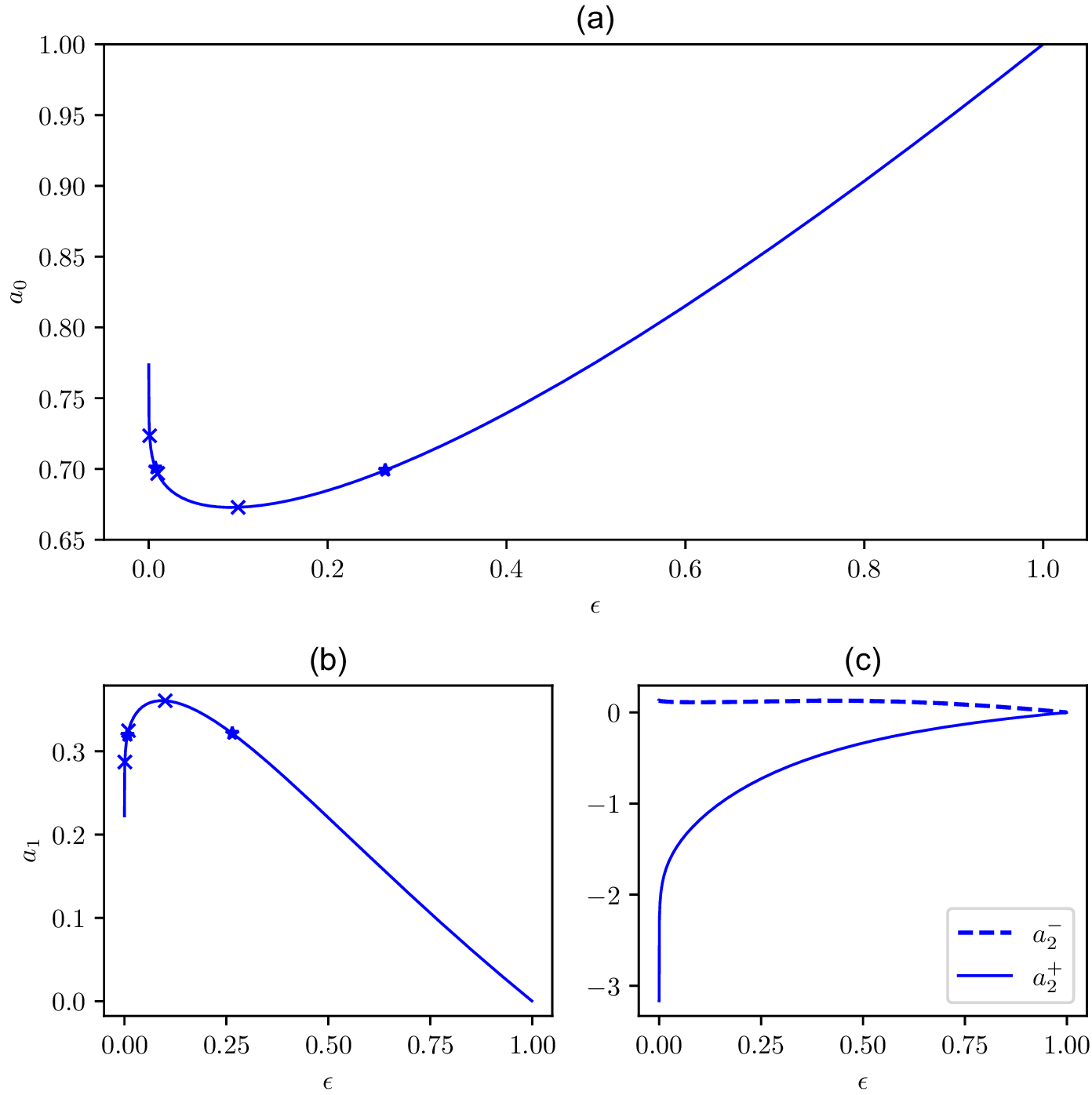
 . In Figure 3, we show how the constants
$a_0$
 and
$a_1$
 depend on
$\epsilon $
 over the range
$\epsilon \in (0,1)$
 . These constants may be considered characteristic parameters describing a solution to the system (1.5), given

where
$x^*_0$
 is the location of the initial discontinuity.
Coefficients from the expansion (2.5) of similarity solutions (2.2) over front height
$\epsilon $
 : (a) the value
$a_0$
 ; (b)
$a_1$
 and (c)
$a_2^\pm $
 . The parameters
$a_0$
 and
$a_1$
 show a turning point, below which
$a_0$
 and
$a_1$
 appear to slowly return to
$1$
 and
$0$
 , respectively. The value of
$a_2^+$
 increases in magnitude (slowly) as
$\epsilon \to 0$
 . The crosses marked on the curves in panels (a,b) correspond to the values
$\epsilon = 10^{-1}, 10^{-2}, 10^{-3}$
 shown in Figure 4(a,b), while the asterisks correspond to the values
$\epsilon = 0.268, 0.0078$
 shown in Figure 4(c,d).

As
$\epsilon $
 decreases, at first
$a_0$
 decreases and
$a_1$
 increases. However, there is a turning point at approximately
$\epsilon = 0.1$
 below which
$a_0$
 begins to increase and
$a_1$
 to decrease. Focusing on small
$\epsilon $
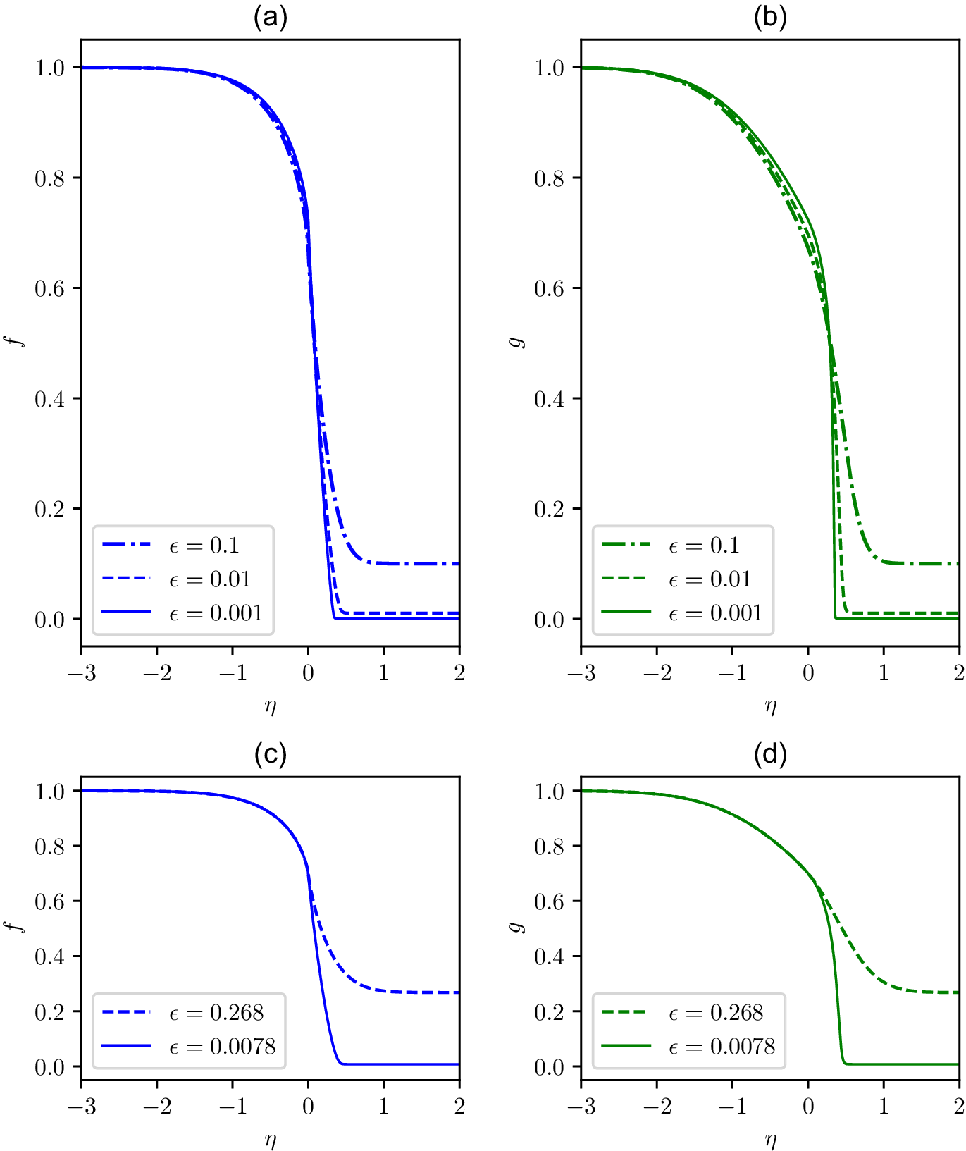
 , in Figure 4(a,b), we plot solution profiles for
$\epsilon = 10^{-1}, 10^{-2}, 10^{-3}$
 . For small
$\epsilon $
 , the similarity solutions are qualitatively different on either side of the singular point
$\eta =0$
 . In particular, the solution profiles are quite flat to the left of the singular point, but to the right, a steep front forms. Close to the bottom of the front, the solution reaches a point where the slopes of both f and g rapidly flatten as f and g approach
$\epsilon $
 . However, the values of
$a_2^\pm $
 differ (see Figure 3(c)), in particular with
$a_2^+ < 0$
 increasing in magnitude as
$\epsilon $
 becomes small. This contrast indicates the magnitude of derivatives of a solution to the left and the right of the singular point become markedly different.
Similarity profiles (a) f and (b) g as
$\epsilon $
 becomes small. An apparent interface at
$\eta =\eta ^*$
 is seen, where the magnitude of f becomes of order
$\epsilon $
 and rapidly flattens out. In panels (c,d), two solutions for different values may have the same value of
$a_0$
 and, thus, the same profile for
$\eta < 0$
 .

The most notable feature for solutions when
$\epsilon $
 is small is the formation of what could be considered an apparent interface at a location
$\eta ^*> 0$
 . This is not a true interface, as for
$\epsilon $
 positive,
$v\to \epsilon $
 never vanishes, but the slope of g appears almost vertical near this point, and the change in slope of f and g occurs very rapidly. In a solution to the PDE (1.5), this apparent interface will occur at
$x^*(t) = x_0^* + \eta ^*t$
 ; thus, the value of
$\eta ^*$
 in the similarity solution represents the speed of propagation of such a point.
To characterize the location of
$\eta ^*$
 over
$\epsilon $
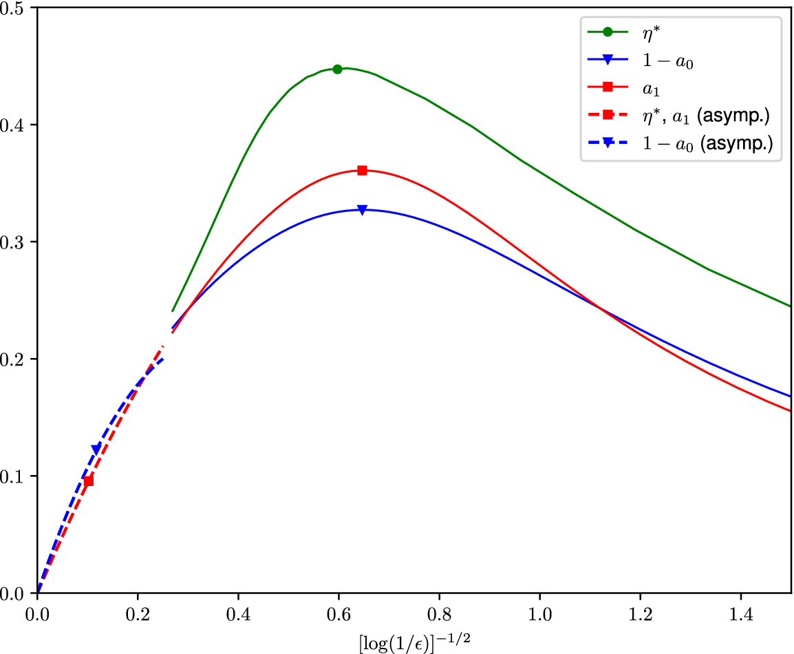
 , we define it as the point at which the slope of g becomes smallest (that is, most negative). In Figure 5, we plot this quantity, along with the difference between
$a_0$
 and its asymptotic value
$1$
 , and the slope
$a_1$
 . As each of these quantities is seen to tend to zero as
$\epsilon \to 0$
 , but slowly, we plot these against the logarithmic variable
$[\log (1/\epsilon )]^{-1/2}$
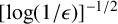 . Here, we see initial signs that these variables are of this logarithmic order as
$\epsilon \to 0$
 , which will motivate the asymptotic analysis in the next section (for comparison, we also plot the results of the asymptotic analysis that we will undertake). Note that in this plot, we take
$\epsilon $
 down to
$10^{-6}$
 , which is at approximately the limit of the numerical solution procedure. For this value,
$[\log (1/\epsilon )]^{-1/2} \approx 0.27$
 is still relatively large, which increases the difficulty of deducing the behaviour in this limit.
Apparent interface location
$\eta ^*$
 , as well as
$1-a_0$
 (where
$a_0 = f(0) = g(0)$
 ) and slope
${a_1 = -g'(0)}$
 , in the limit where
$\epsilon $
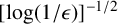
 becomes small. Numerical results indicate that these solution parameters are all going to zero, although only logarithmically fast, namely, of order
$[\log (1/\epsilon )]^{-1/2}$
 as
$\epsilon \to 0$
 . Also plotted are the two-term asymptotic approximations (3.12) for each parameter (note these approximations are valid in the limit
$\epsilon \to 0$
 ).

Finally, we note some interesting implications of the nonmonotonic nature of the constants
$a_0$
 and
$a_1$
 seen in Figure 3. One implication, which can be seen in the small
$\epsilon $
 solution in Figure 4(a,b), is that a smaller value of
$\epsilon $
 to the right of the singular point may result in a larger value of g (and thus v) to the left of the singular point. This means that given initial conditions for which the diffusivity u vanishes, the problem (1.5) does not necessarily satisfy a comparison principle; one may have two solutions
$v_1$
 and
$v_2$
 , where
$v_1 \leq v_2$
 at
$t=0$
 , but
$v_1$
 does not remain bounded by
$v_2$
 for
$t> 0$
 .
The profile to the left of
$\eta =0$
 is uniquely characterized by
$a_0$
 , as for a given
$a_0$
 , both
$a_1$
 and
$a_2^-$
 are determined by requiring the
$\eta \to -\infty $
 condition to be met. A second implication of nonmonotonic
$a_0$
 is thus that two different values of
$\epsilon $
 can result in two similarity solutions that are identical for
$\eta <0$
 , while being distinct for
$\eta> 0$
 . In Figure 4(c, d), we plot the similarity solutions for
$\epsilon \approx 0.268$
 and
$\epsilon \approx 0.0078$
 , both corresponding to a value of
$a_0 = 0.7$
 . Here, we see the exact agreement for
$\eta < 0$
 . Given the similarity solutions represent exact solutions of the PDE, this implies that two initial conditions to (1.5) which are the same on one side of the singular point
$x = x^*_0$
 could remain the same for
$t>0$
 , even if this is not the case on the other side of the singular point.
3 Asymptotic analysis for small
$\epsilon $

As indicated by the numerical solutions, solution characteristics, including the apparent interface location
$\eta ^*$
 , appear to very slowly (logarithmically) tend to zero as the front height
$\epsilon $
 vanishes. In this section, we establish this result systematically using a matched asymptotic analysis.
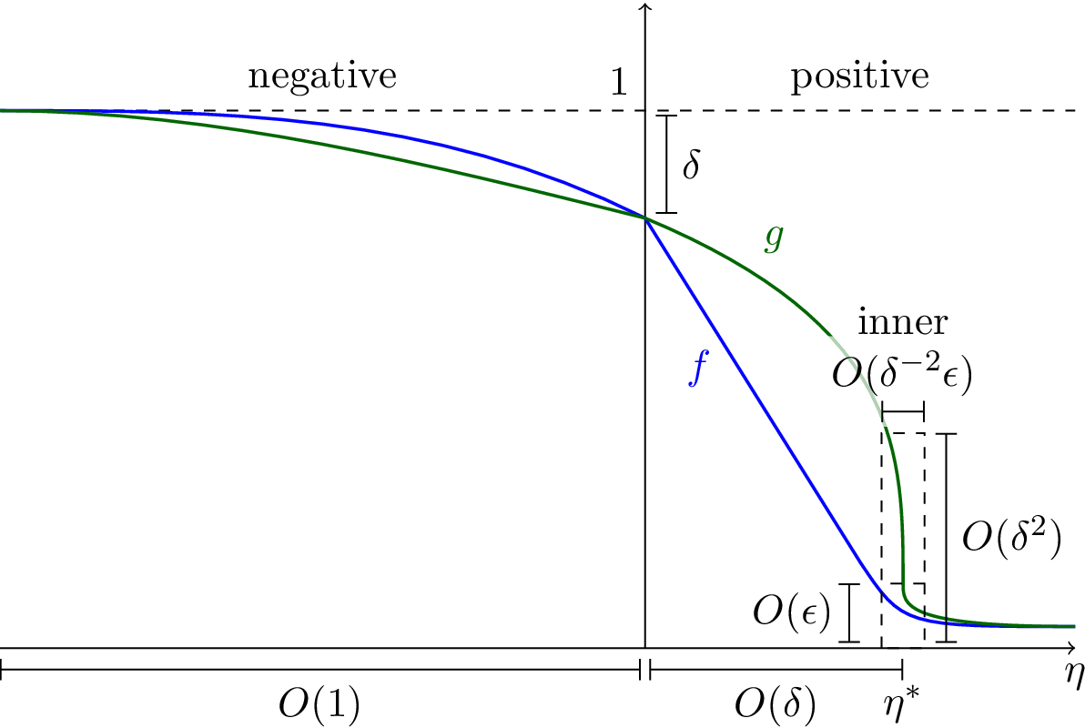
In Figure 6, we sketch an overview of the asymptotic structure that we uncover in this section. The structure of the solution profiles in the small-
$\epsilon $
 limit are starkly different for
$\eta < 0$
 left of the singular point, and
$\eta> 0$
 to the right. For
$\eta < 0$
 , both f and g become close to flat, whereas for
$\eta> 0$
 , the solution profiles are compressed in a region
$0 < \eta < \eta ^*$
 , which becomes logarithmically small in the limit
$\epsilon \to 0$
 . Finally, there is an inner boundary layer problem close to
$\eta ^*$
 that must be resolved and matched to the outer region to determine the relationship between each solution parameter.
Schematic of the asymptotic structure of similarity solutions to (2.2) as described in Section 3. The solution has three main regions: the negative region
$\eta < 0$
 , the positive region
$0 < \eta < \eta ^*$
 (where
$\eta ^*$
 is the apparent front location) and an inner region close to
$\eta ^*$
 . Matching in the inner region reveals that
$\delta = O(\log (1/\epsilon )^{-1/2})$
 .

We start by defining a small parameter
$\delta $
 , by

As seen in Figure 5, we expect
$\delta $
 to be logarithmically small as
$\epsilon $
 vanishes; the goal of the asymptotic analysis will be to determine this relationship precisely. We will calculate as many terms as required to find two terms in the series approximation of
$\delta (\epsilon )$
 . Higher terms quickly become infeasible due to the complexity of the integrations required.
3.1 Negative
$\eta $

When
$\eta < 0$
 , the profiles f and g are both constrained in magnitude by the far-field condition
$f, g \to 1$
 as
$\eta \to -\infty $
 . Given the definition (3.1), we assume the asymptotic expansion

Substituting into the ODE system (2.2) and taking successive terms in
$\delta $
 , we have

and so on, with each
$f_j$
 found from
$g_j$
 by integrating

To satisfy the far-field condition, we require
$f_j, g_j\to 0$
 as
$\eta \to -\infty $
 , while from the definition of
$\delta $
 ,

We thus have

where
$\operatorname {\mathrm {erf}}$
 is the error function and
$\operatorname {\mathrm {Ei}}$
 is the exponential integral, defined for negative arguments by

The next term
$g_2$
 is complicated but is possible to find explicitly by integrating

The derivative of
$g_2$
 at
$\eta =0$
 is needed to give the correction to the slope
$a_1$
 that matches with that for
$\eta>0$
 . Differentiating the above, we find that

where

3.2 Positive
$\eta $
away from apparent interface

We now consider the interval
${0 < \eta < \eta ^*}$
 , where
$\eta ^*$
 is the apparent interface location. Since
$\eta ^*$
 is seen to decrease at the same logarithmic rate as
$\delta $
 , we introduce the scaled independent variable
$\xi $
 by
$\eta = \delta \xi $
 , so that (2.2) becomes

We take the apparent interface location
$\eta ^* = \delta \xi ^*$
 , where
$\xi ^*$
 has a series expansion in
$\delta $
 :

Expanding the similarity profiles f and g in this region as

the first terms must satisfy the differential equations

At
$\xi =0$
 , the value and derivative of g must match with those for
$\eta \to 0^-$
 , giving the boundary conditions

Another boundary condition comes from the apparent interface at
$\xi ^*$
 . We expect f to be exponentially small in
$\delta $
 close to this point, so expanding
$\xi ^*$
 and f, each term in
$\delta $
 must vanish:

This set of equations and boundary conditions implies that
$f_0$
 and
$f_1$
 are linear, while
$g_0$
 and
$g_1$
 are constant:

We can continue to higher terms. We will calculate the next corrections
$g_2$
 and
$g_3$
 , which satisfy

with boundary conditions

Note that the higher corrections to f are not required to calculate g to this order. Integrating and applying the conditions at zero, we find


3.3 Inner problem near apparent interface
The expansions (3.5) and (3.6) are singular in the limit
$\xi \to \xi ^*$
 . There is thus a region close to
$\xi =\xi ^*$
 where the solution will match onto an inner solution, in which the far-field condition
$f \to \epsilon $
 is attained. We thus define inner variables z,
$\hat f$
 and
$\hat g$
 by

Here, the scale of f is determined so that
$\hat f \to 1$
 as
$z\to \infty $
 , while the scales for z and g are determined by finding the appropriate balance of terms in (3.4). Under this change of variables, the system (3.4) is, to leading order,

Note that a result of solving the system in a small region near
$\xi ^*$
 is that the system is autonomous. Solutions of (3.7) are effectively travelling wave solutions of (1.5); this inner problem is thus relevant close to an apparent interface not just for the similarity solution, but in more general contexts (see further discussion in Section 4).
To match to the far-field condition, we require
$\hat f \to 1$
 ,
$\hat f' \to 0$
 as
$z\to \infty $
 . Integrating (3.7) twice and applying these conditions, we find

thus, we have an implicit solution as follows:

where
$z_0$
 is an arbitrary translational constant and
$\operatorname {\mathrm {li}}$
 is the logarithmic integral. Note that
$\hat g$
 vanishes in the limit
$z \to \infty $
 , which is consistent with the definition of
$\hat g$
 given
$\delta ^2 \gg \epsilon $
 ; an additional inner problem would be required to match g onto its far-field condition
$g \to \epsilon $
 .
What remains is to find the asymptotic relationship between
$\delta $
 and
$\epsilon $
 , as well as the asymptotic formula for the apparent interface location
$\xi ^*$
 . To do so, we need to match the
$z\to -\infty $
 expansion of the inner problem (3.9) to the
$\xi \to \xi ^*$
 expansion of the outer problem (3.5), (3.6).
While the asymptotic expansion for the inverse logarithmic integral could be applied directly to (3.9), a simpler way to carry out the matching is to write the relationship between
$\hat g$
 and
$\hat f$
 in (3.9) in terms of the outer variables, giving

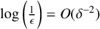
To have an
$O(1)$
 term on the right of (3.10) to match that on the left, we require
$\log \bigg (\frac {1}{\epsilon }\bigg ) = O(\delta ^{-2})$
 . Thus, we let

Substituting these expansions into (3.10), along with those for f and g, (3.5), (3.6), we have from each order:


Here, the constant terms in the latter two equations involve higher order corrections (
$\xi ^*_2$
 ,
$\ell _2$
 and so forth).
The terms in the expansions for
$\xi _0$
 and
$\log ({1}/{\epsilon })$
 are now found as follows. The constants
$\xi _0^*$
 and
$\xi _1^*$
 are found by comparing the logarithmic terms in (3.11)(c,d) with those in (3.6). The more singular term in
$g_3\, \propto f_0^{-1}$
 then matches automatically. The constants
$\ell _0$
 and
$\ell _1$
 are then found by comparing the constant terms in (3.11)(a,b) to (3.5). We thus find

where
$a_{11}$
 and
$a_{12}$
 are the terms in the expansion of the slope at
$\eta =0$
 (3.3).
Finally, since
$\epsilon $
 is the independent parameter of the original problem, we invert the series expansions to find the front at
$\eta ^* = \delta \xi ^*$
 . Thus,


Note that the expansions for the front location,
$\eta ^*$
 , and the slope at zero,
$a_1$
 , are the same to this order.
3.4 Comparison with numerical results
We of course want to compare the above asymptotic result with the numerical results of Section 2. We plot the expansions (3.12) in Figure 5 along with the numerical calculations of the same quantities. The logarithmic dependence of the solution parameters on
$\epsilon $
 is certainly consistent with their observed numerical behaviour, even if the agreement is not very close at the level that we can achieve numerically. A major challenge in comparing the asymptotic solution directly to numerical results is the slow convergence of the logarithmic terms. For
$\epsilon = 10^{-6}$
 , which is around the smallest value we can attain with our numerical method,
$[\log ({1}/{\epsilon })]^{-1/2} \approx 0.27$
 , which is not very small. At this value, the correction terms in the asymptotic formulae (3.12) do improve the leading order result. For
$\epsilon = 10^{-6}$
 , the leading order asymptotic estimates of
$\delta $
 in (3.12a) and
$\eta ^*$
 in (3.12b) are respectively

Including the
$O([\log ({1}/{\epsilon })]^{-1})$
 correction terms leads to estimates
$\delta \approx 0.206$
 and
${\eta ^* \approx 0.224}$
 . By comparison, the values estimated from the numerical solution in Section 2.3 are

However, by using the numerical estimates for
$\delta $
 and
$\eta ^*$
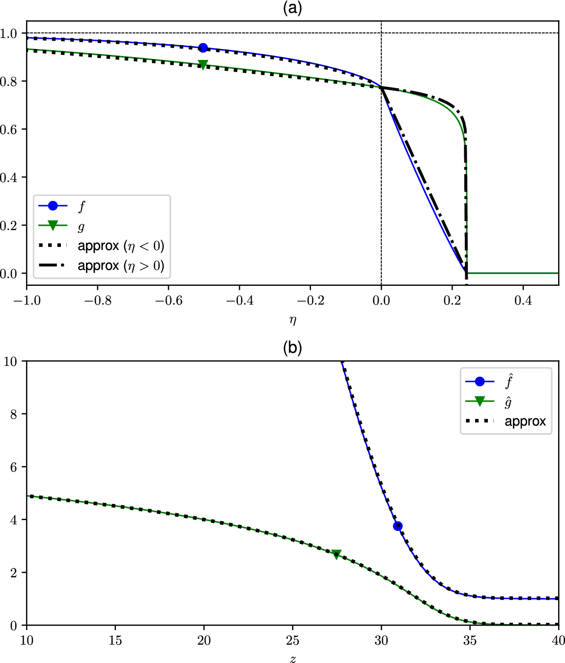
 in (3.13) instead of asymptotic approximations, we can find encouraging agreement with the solution profiles in each region. In Figure 7(a), we plot the asymptotic solution for
$\eta < 0$
 and
$0 < \eta < \eta _0$
 . Here, we use the
$O(\delta )$
 expansions (3.2a) for
$\eta < 0$
 , and for
$\eta> 0$
 , we use the approximations for f and g that satisfy the conditions at
$\eta =0$
 and include their first nonuniform terms, that is,

(a) Comparison between the numerically computed similarity solution with
$\epsilon =10^{-6}$
 , and approximate profiles given by (3.2a) for
$\eta < 0$
 and (3.14). Due to the very slow convergence of the logarithmic terms as
$\epsilon \to 0$
 , numerical estimates of
$\delta $
 and
$\eta ^*$
 are used in fitting these profiles. (b) Asymptotic and numerical profiles in the inner region near
$\eta ^*$
 . Since the asymptotic solution is accurate to
$O(\epsilon )$
 in this region, the agreement is excellent.

In Figure 7(b), we compare the solution close to
$\eta ^*$
 , scaled into variables z,
$\hat f$
 and
$\hat g$
 , with the inner solution (3.9). To do so, we also have to numerically estimate the translational constant
$z_0$
 (this constant is exponentially small in
$\delta $
 , so in terms of the asymptotic analysis, cannot not be estimated from matching to any finite number of terms of the outer problem). Otherwise, the agreement is practically perfect, which is to be expected given the error in the inner region is of order
$\epsilon $
 , rather than
$\delta $
 .
4 Discussion
Our main finding in this study is the singular nature of the limit of a system that couples degenerate diffusion and degradation of the surrounding environment, as we attempt to approach a system that could exhibit a moving interface (that is, a point where the diffusivity vanishes). The fact that the speed of propagation vanishes in this limit, and gradients of the solution become infinite, is strong evidence that the system cannot exhibit such a moving interface.
The analysis undertaken for the idealized system (1.5) is also relevant for more complex models of the form (1.3) for which coupled degenerate diffusion and degradation is the driving factor. Consider a model of the form (1.3) with
$F(\tilde u)$
 such that
$F(1) = 0$
 , starting at a piecewise-constant initial condition such as (1.6). For early times, we may use the same similarity scaling as (2.1), which will then be the leading order behaviour of solutions for small t, that is,

The effect of the reaction terms, as well as the diminishing decay of
$\tilde u$
 as
$\tilde u$
 itself decreases, induces an
$O(t)$
 correction to the leading order solution, which is the same similarity solution as considered in this study. More generally, we expect the inner problem (3.8) to be the relevant inner problem near any apparent moving interface (not just in the context of a similarity solution), so that the logarithmic dependence of speed on a regularization of order
$\epsilon $
 near the apparent front will hold in other contexts, for example, travelling wave solutions. We also note that for early times, the same similarity solution will hold near a step discontinuity in versions of (1.3) posed in higher spatial dimensions.
The logarithmic dependence of speed on the small parameter
$\epsilon $
 explains previous observations made chiefly from PDE simulations in the literature [Reference Colson, Sánchez-Garduño, Byrne, Maini and Lorenzi8, Reference El-Hachem, McCue and Simpson15, Reference Mascia, Moschetta and Simeoni21]. It is not surprising that numerical methods applied to systems of the form (1.3) with an initially compactly supported condition will appear to evolve in time with a well-defined front. In a numerical scheme,
$\epsilon $
 is representative of the mesh size of the spatial discretization. It is very challenging in a discretized PDE simulation to obtain a mesh size less than
$\sim 10^{-3}$
 or so, and for such a value of
$\epsilon $
 , the apparent speed of propagation of a front (including, for example, the apparent speed of a travelling wave) will appear to be a positive quantity. The careful examination of the convergence of numerical simulations, as was done in [Reference Mascia, Moschetta and Simeoni21], for example, is thus crucial for these forms of degenerate diffusion systems.
While we have considered the regularizing parameter
$\epsilon $
 as the height in front of an evolving profile, it could be considered equivalent to a number of regularizations that will produce similar results. For example, in a continuum limit of a discrete process (for example, an agent based model of individual cells), the (nondimensional) individual cell size could be considered a small but nonzero regularizing parameter. In each case, the details of the
$O(\epsilon )$
 inner problem near an apparent interface would be different, but the matching with the outer problem would result in the same logarithmic dependence.
The regularizing effect of height
$\epsilon $
 near a moving front has interesting parallels to the contact-line paradox in interfacial fluid dynamics, in which the classical laws of hydrodynamics (in particular, the no-slip boundary condition) cannot model the motion of contact line in the spreading of a droplet, for instance, [Reference Huh and Scriven19]. In such cases, a number of regularizations (such as disjoining pressure or Navier slip) are posited that regularize the singularity at the contact line and the contact line speed is logarithmically dependent on the small parameter in the regularization [Reference Bonn, Eggers, Indekeu, Meunier and Rolley4, Reference Snoeijer and Andreotti26].
Another example of logarithmic dependence on a small regularization from mathematical biology is the effect of perturbing the reaction term in the Fisher–KPP equation on its travelling wave speed, for example, the cut-off effect considered in [Reference Brunet and Derrida6, Reference Dumortier, Popović and Kaper14]. Here, the perturbation is introduced to take into account the discrete size of cells. Although the limit is not singular in this case (the standard minimum Fisher–KPP travelling wave is recovered in the limit), the effect on the wave speed is logarithmic and so can deviate significantly from that expected.
We now consider some possible extensions of this work. The similar class of cross-diffusion models considered [Reference Crossley, Maini, Lorenzi and Baker9, Reference Crossley, Pietschmann and Schmidtchen10, Reference Simpson, Murphy, McCue and Buenzli25], which may, at least in an idealized form, be represented by the system

for some function
$\phi (v)$
 . For an initially piecewise condition such as (1.6), a system of this form will also be amenable to a similarity scaling similar to that carried out in this study. We foresee such systems having the same logarithmic dependence on any regularization near an apparent interface, although the details of the similarity solution will depend on the form of
$\phi $
 .
Finally, if one wanted a system similar to (1.5) that allowed for actual moving interfaces, one approach could be to weaken the degeneracy of the diffusivity by introducing a power-law relationship:

where the exponent
$m \in (0,1)$
 . This alteration is likely to allow for (weak) solutions with moving interfaces, as if we expand solutions of (4.1) close to an interface
$x^*(t)$
 where u and v both vanish, we find a valid balance:

where the velocity of the interface
$\dot x_0^* = (1-m)A^m/m$
 . Of course, these terms are clearly singular in the limit
$m\to 1^-$
 as we approach the original system (1.5). We will consider such problems in future studies.













 Open access

