1 Introduction
Shock/turbulent-boundary-layer interactions (STBLIs) occur in a variety of high-speed flows, including inlet, internal propulsion and external control surface applications. The pressure rise across strong interactions induces flow separation, which introduces new mechanisms of unsteadiness to the flow, with prominent fluctuations at frequencies less than those associated with the undisturbed turbulent boundary layer (Dolling Reference Dolling2001). This unsteadiness is undesirable in many aerospace applications, because it can result in extreme thermo-mechanical loading of surfaces, reduced propulsion efficiency, degraded control authority and disruptive optical aberration. Recent developments and remaining fundamental challenges in this area are discussed by Clemens & Narayanaswamy (Reference Clemens and Narayanaswamy2014) and Gaitonde (Reference Gaitonde2015).
Significant advancement toward the understanding of unsteadiness in spanwise-homogeneous (nominally two-dimensional: 2-D) STBLIs has been achieved recently through the application of high-fidelity simulations (see e.g. Morgan et al. Reference Morgan, Duraisamy, Nguyen, Kawai and Lele2013) and high-resolution measurement techniques (e.g. Souverein et al. Reference Souverein, Van Oudheusden, Scarano and Dupont2009) to the problem. Across a variety of flow conditions, the peak frequency ( $f$) representative of the lowest band of unsteadiness has been demonstrated to scale well with Strouhal number
 $(St_{L}=fU_{\infty }/L)$ based on the free-stream velocity
 $(U_{\infty })$ and separation length
 $(L)$ (Dupont, Haddad & Debiève Reference Dupont, Haddad and Debiève2006). For flow conditions of interest in aerospace applications, this peak of the low-frequency band is typically realized two decades below that of the band describing fluctuations of the undisturbed boundary layer (Dussauge, Dupont & Debiève Reference Dussauge, Dupont and Debiève2006). A variety of explanations have been examined to describe the mechanism of this low-frequency unsteadiness. Some place emphasis on the upstream forcing of the interaction (Beresh, Clemens & Dolling Reference Beresh, Clemens and Dolling2002; Ganapathisubramani, Clemens & Dolling Reference Ganapathisubramani, Clemens and Dolling2009; Porter & Poggie Reference Porter and Poggie2019), others the dynamics of the separation (Piponniau et al. Reference Piponniau, Dussauge, Debiève and Dupont2009), downstream Görtler-like forcing (Priebe et al. Reference Priebe, Tu, Rowley and Martín2016), the filtering behaviour of the interaction (Touber & Sandham Reference Touber and Sandham2011), the oscillator behaviour (Plotkin Reference Plotkin1975) or the absolute instability of the flow (Touber & Sandham Reference Touber and Sandham2009; Pirozzoli et al. Reference Pirozzoli, Larsson, Nichols, Bernardini, Morgan and Lele2010; Nichols et al. Reference Nichols, Larsson, Bernardini and Pirozzoli2017).
Our understanding of the 2-D STBLI low-frequency mechanism has been recently documented (Adler & Gaitonde Reference Adler and Gaitonde2018a), in which unsteadiness in the low-frequency band is described as resulting from a nonlinear oscillator, which is intrinsic to the STBLI and driven subject to nonlinear forcing. The flow was shown to admit an absolute instability, with linear restoring behaviour at extreme shock displacement, not inconsistent with the premise of the linear oscillator description (Plotkin Reference Plotkin1975). However, the behaviour of the absolute instability was shown to be asymmetric with respect to the mean shock position, with behaviour of the instability at the mean shock position promoting upstream motion, consistent with the zero-frequency mode uncovered from 2-D stability analyses (Touber & Sandham Reference Touber and Sandham2009; Pirozzoli et al. Reference Pirozzoli, Larsson, Nichols, Bernardini, Morgan and Lele2010; Nichols et al. Reference Nichols, Larsson, Bernardini and Pirozzoli2017). Because of this asymmetry, the oscillator is necessarily nonlinear, with forcing necessarily dependent on the position of the shock. To account for the limit cycle stability of the STBLI, there must be a bias in the nonlinear forcing in the downstream direction to counter the linear upstream bias; this nonlinear downstream bias agrees with the mass-depletion mechanism of Piponniau et al. (Reference Piponniau, Dussauge, Debiève and Dupont2009). Further, as discussed by Touber & Sandham (Reference Touber and Sandham2011), any such oscillator description (like that which we have proposed) promotes low-frequency filtering of external upstream (Ganapathisubramani et al. Reference Ganapathisubramani, Clemens and Dolling2009; Poggie Reference Poggie2019; Porter & Poggie Reference Porter and Poggie2019) or downstream (Piponniau et al. Reference Piponniau, Dussauge, Debiève and Dupont2009; Priebe et al. Reference Priebe, Tu, Rowley and Martín2016) disturbances. The resulting mechanism (Adler & Gaitonde Reference Adler and Gaitonde2018a) unifies aspects of several major trains of thought, each conjoined in a very complex interdependent process, in which causation and correlation often remain difficult to distinguish from each other. It should be noted that the aforementioned stability analyses of the turbulent mean flow (Touber & Sandham Reference Touber and Sandham2009; Pirozzoli et al. Reference Pirozzoli, Larsson, Nichols, Bernardini, Morgan and Lele2010; Nichols et al. Reference Nichols, Larsson, Bernardini and Pirozzoli2017) identify the instability of the unsteady equations about the turbulent mean flow with no Reynolds-averaged Navier–Stokes-like Reynolds stress, whereas a stability analysis including a Reynolds stress term (Crouch, Garbaruk & Magidov Reference Crouch, Garbaruk and Magidov2007), would merit interpretation from a different perspective, which should also be pursued (Crouch, Garbaruk & Strelets Reference Crouch, Garbaruk and Strelets2019; Timme Reference Timme2019).
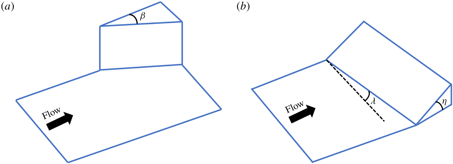
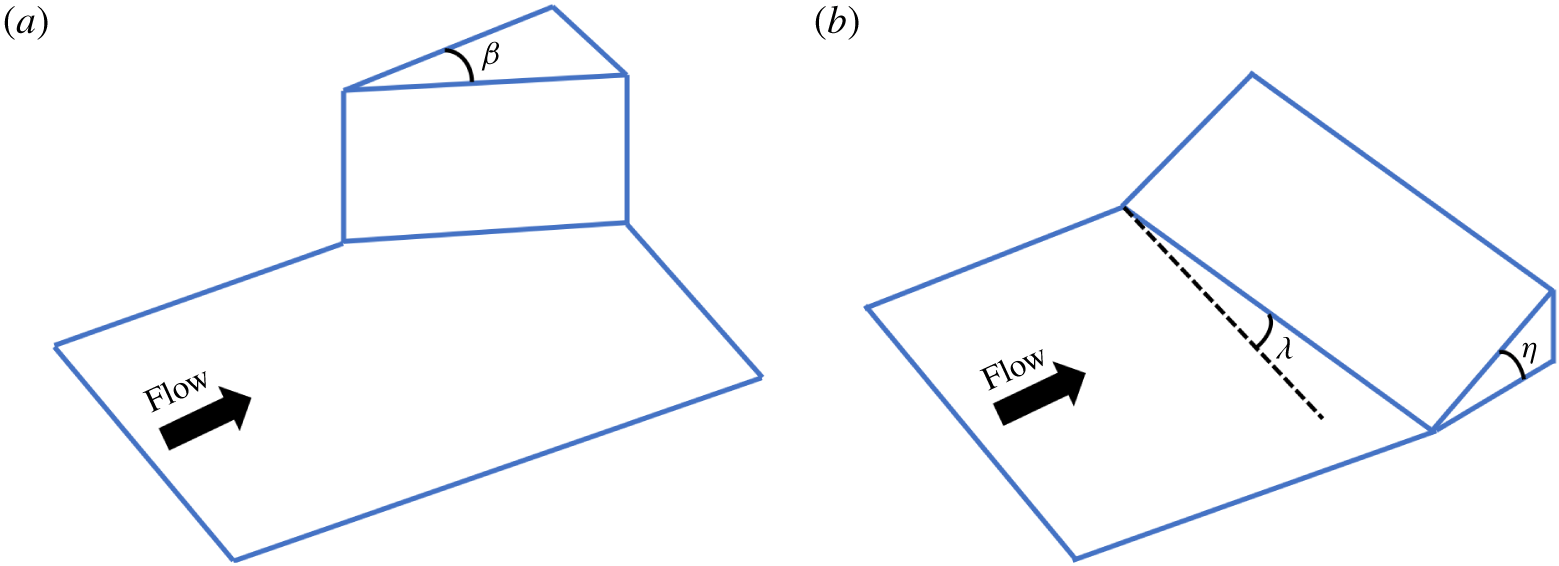
The description of unsteadiness in 3-D STBLIs – specifically, those in which the shock generator(s) are swept with respect to the incoming flow (Zheltovodov & Knight Reference Zheltovodov, Knight, Babinsky and Harvey2011) – has not yet been developed to the same extent as that for 2-D interactions. Several canonical configurations have been proposed to isolate the key features of interest in these interactions; among these, the sharp fin (SF; figure 1a) and swept compression ramp (SCR; figure 1b) are chosen in this study as representatives. The former is characterized by the angle of attack,  $\unicode[STIX]{x1D6FD}$, while the latter requires two specifications: a sweep angle,
 $\unicode[STIX]{x1D706}$ and a compression angle,
 $\unicode[STIX]{x1D702}$. These strong, swept, 3-D STBLIs, are relevant in many aerospace applications, and affect crucial phenomena both internally (e.g. total pressure recovery in sidewall-compression inlets (Gruhn & Gülhan Reference Gruhn and Gülhan2011; Nguyen et al. Reference Nguyen, Behr, Reinartz, Hohn and Gülhan2013)) and externally (e.g. shock-induced flow separation for delta-wing configurations (Miller & Wood Reference Miller and Wood1984; Donohoe & Bannink Reference Donohoe and Bannink1997)). As such, recent efforts have refocused examination from 2-D configurations toward these swept STBLIs (Adler & Gaitonde Reference Adler and Gaitonde2018b; Mears, Arora & Alvi Reference Mears, Arora and Alvi2018; Vanstone et al. Reference Vanstone, Musta, Seckin and Clemens2018). However, there are significant structural differences between 2-D and 3-D interactions which suggest that the flow structure and underlying mechanisms (including those associated with unsteadiness) in 2-D interactions cannot be directly extended to three dimensions. These differences follow from the quasi-conical symmetry of 3-D interactions, in which the symmetry of the mean flow is realized through the approximate collapse of profiles plotted in spherical coordinates centred on a virtual conical origin (VCO) (Settles & Kimmel Reference Settles and Kimmel1986). Visually, these interactions exhibit separation, attachment, and shock-triple-point lines that outline a conical structure, with each line emanating from the cone apex, which is located at the VCO. A consequence of this symmetry is that the separation length becomes a local (not global) property of the flow; in three dimensions, the local separation arc-length grows linearly with displacement from the VCO. This limits the extendibility of the
 $St_{L}$ scaling, which is effective in describing prominent low-frequency unsteadiness in 2-D interactions (Dupont et al. Reference Dupont, Haddad and Debiève2006), to the more general 3-D interactions.
Principal swept configurations examined: SF (a) and SCR (b).  $\unicode[STIX]{x1D6FD}$ = angle of attack;
 $\unicode[STIX]{x1D706}$ = angle of sweep;
 $\unicode[STIX]{x1D702}$ = angle of compression.
Indeed, the separation topology for 3-D STBLIs is more aptly treated in a local, rather than global, framework. For 3-D separation, streamlines of the separating flow do not necessarily reattach (Gaitonde, Shang & Visbal Reference Gaitonde, Shang and Visbal1995), and the separation surface topology is more suitably described in terms of singular points (Chapman & Yates Reference Chapman and Yates1991), as opposed to global lines of separation and reattachment, as is convenient in two dimensions. Consequently, in 3-D STBLIs, there is no recirculation in the strict sense, in which streamlines of the mean-flow feed back onto themselves (Panaras Reference Panaras1996). This observation is linked to the lack of topological separation closure in simple, swept, 3-D interactions; the separation is not closed, in that it is initiated by an attachment-node/separation-saddle pair, but a closing separation-node/saddle pair cannot be realized without breaking the conical symmetry of the interaction (Adler & Gaitonde Reference Adler and Gaitonde2019a). This differs from the separation observed in confined 2-D STBLIs, which are necessarily topologically closed near the sidewalls by additional separation-node/saddle pairs (Poggie & Porter Reference Poggie and Porter2019; Rabey et al. Reference Rabey, Jammy, Bruce and Sandham2019; Xiang & Babinsky Reference Xiang and Babinsky2019) (an example of type-2 separation (Chapman & Yates Reference Chapman and Yates1991)); otherwise, for 2-D interactions, a semi-infinite wind tunnel or spanwise-periodic simulation domain effectively closes the separation through 2-D degeneracy (Green Reference Green1970a).
The mean-flow features of several canonical swept 3-D interactions were well documented throughout the 1980s and 1990s as a result of both experimental (Settles & Dolling Reference Settles, Dolling, Nielsen and Hemsch1986, Reference Settles and Dolling1990; Settles et al. Reference Settles, Degrez, Knight, Dolling, Delery, Vandromme and Simeonides1993) and numerical (Reynolds-averaged Navier–Stokes: RANS-based) efforts (Panaras Reference Panaras1996; Knight et al. Reference Knight, Yan, Panaras and Zheltovodov2003), and flow models were proposed for the SF (Knight et al. Reference Knight, Badekast, Horstman and Settles1992a), SCR (Knight, Horstman & Bogdonoff Reference Knight, Horstman and Bogdonoff1992b) and double-fin (DF) (Gaitonde et al. Reference Gaitonde, Shang and Visbal1995) interactions. These efforts yielded significant insight into the mean-flow structure, and although some studies documented unsteadiness via time-resolved surface pressure measurements (Schmisseur & Dolling Reference Schmisseur and Dolling1992; Erengil & Dolling Reference Erengil and Dolling1993; Schmisseur & Dolling Reference Schmisseur and Dolling1994), these were inhibited from providing a full basis for the spatio-temporal characterization, because the technologies of time-resolved particle-image velocimetry (PIV) and high-fidelity large-eddy simulation (LES) were not yet fully mature. This technological barrier is now essentially overcome, which facilitates a reexamination of these flows with the goal of understanding the phenomenology and underlying mechanisms of unsteadiness.
In addition to the commonly discussed ‘low-frequency’  $(St_{\unicode[STIX]{x1D6FF}}\lesssim 0.01)$ unsteadiness (two decades below the characteristic boundary-layer frequency,
 $St_{\unicode[STIX]{x1D6FF}}=1$, with outer-scale boundary-layer thickness,
 $\unicode[STIX]{x1D6FF}$), another mechanism of unsteadiness has been demonstrated in 2-D STBLIs; this mechanism relates to mean flow gradients in the post-separation shear layers, and the development of unsteady (mid-frequency:
 $St_{\unicode[STIX]{x1D6FF}}\sim 0.1$) coherent fluctuations in these shear layers. These are akin to the wave-induced (middle) component of the triple decomposition (Reynolds & Hussain Reference Reynolds and Hussain1972), and the peak frequency of this mid-frequency band is typically realized one decade below the peak of the band describing fluctuations of the undisturbed boundary layer (Agostini et al. Reference Agostini, Larcheveque, Dupont, Denieve and Dussauge2012). Coherent mid-frequency fluctuations in the shear layers of 2-D STBLIs have been described in several experimental (Souverein et al. Reference Souverein, Van Oudheusden, Scarano and Dupont2009, Reference Souverein, Dupont, Debiève, Van Oudheusden and Scarano2010) and numerical (Agostini et al. Reference Agostini, Larcheveque, Dupont, Denieve and Dussauge2012; Aubard, Gloerfelt & Robinet Reference Aubard, Gloerfelt and Robinet2013; Nichols et al. Reference Nichols, Larsson, Bernardini and Pirozzoli2017; Adler & Gaitonde Reference Adler and Gaitonde2018a) investigations. These fluctuations are convective, vortical in nature and their passage through the interaction correlates with rippling/corrugation of the shock (Agostini et al. Reference Agostini, Larcheveque, Dupont, Denieve and Dussauge2012). Their development begins in the separated shear layer (Souverein et al. Reference Souverein, Dupont, Debiève, Van Oudheusden and Scarano2010; Aubard et al. Reference Aubard, Gloerfelt and Robinet2013), and is reflective of underlying Kelvin–Helmholtz-like instabilities. The coupling between these mid-frequency fluctuations and low-frequency dynamics is an active area of interest (Agostini, Larchevêque & Dupont Reference Agostini, Larchevêque and Dupont2015; Bonne et al. Reference Bonne, Brion, Garnier, Bur, Molton, Sipp and Jacquin2019).
However, the aforementioned significant differences between the spanwise-homogeneous shear-layer symmetry in 2-D interactions and the quasi-conical shear-layer symmetry in 3-D interactions has ramifications for the mid-frequency coherent fluctuations developing within these shear layers. While inviscid supersonic flow past a swept shock generator results in a perfectly conically symmetric flow field (3-D), the corresponding viscous flow results in quasi-conical symmetry, in part, due to the spanwise-homogeneous nature of the incoming boundary layer, which introduces a new, finite, 2-D length scale to the flow (the boundary-layer thickness), uniformly across the span. A conflict then naturally arises as a result of the competing 2-D and 3-D similarity scaling parameters. In 2-D supersonic separation, the classical free-interaction principle (Chapman, Kuehn & Larson Reference Chapman, Kuehn and Larson1957) describes the independence of the early stages of separation from the downstream flow properties (e.g. the nature of the shock generator), and this scaling applies reasonably well to the early stages of separation in 2-D STBLIs (Green Reference Green1970b). Alternatively, the 3-D free-interaction principle (Settles & Kimmel Reference Settles and Kimmel1986), makes a similar argument for conical symmetry in 3-D STBLIs, in that the separation responds to the 3-D (conical) footprint of the free-stream ‘pseudo-inviscid’ interaction. Recent results (Adler & Gaitonde Reference Adler and Gaitonde2019a) suggest that the mean-flow similarity scaling of the quasi-conical shear layers in 3-D STBLIs exhibit a mix between 2-D and 3-D free-interaction scaling; however, the ramifications of this mean-flow scaling on mid-frequency unsteadiness have not yet been described.
This current work is part of a series of recent efforts, composed of joint high-resolution experiments and high-fidelity simulations, to understand the unsteady dynamics of strong, swept, 3-D STBLIs. These thrusts have been prompted by several recent advances in massively parallel simulations (Poggie, Bisek & Gosse Reference Poggie, Bisek and Gosse2015) as well as time-resolved unsteady measurements of high-speed flows (Beresh et al. Reference Beresh, Kearney, Wagner, Guildenbecher, Henfling, Spillers, Pruett, Jiang, Slipchenko and Mance2015) and other novel measurement techniques (Fahringer & Thurow Reference Fahringer and Thurow2018). The effort combines experimental measurements of the SCR (Vanstone et al. Reference Vanstone, Saleem, Seckin and Clemens2016, Reference Vanstone, Musta, Seckin and Clemens2018) and SF (Baldwin et al. Reference Baldwin, Arora, Kumar and Alvi2016; Jones et al. Reference Jones, Clifford, Bolton, Thurow, Mears and Alvi2017; Arora et al. Reference Arora, Ali, Zhang and Alvi2018) interactions, along with high-fidelity large-eddy simulations (Adler & Gaitonde Reference Adler and Gaitonde2017, Reference Adler and Gaitonde2018b, Reference Adler and Gaitonde2019a,Reference Adler and Gaitondeb) of both configurations. The swept-impinging-shock (SIS) interaction is also of great interest, and is the subject of parallel experimental (Doehrmann et al. Reference Doehrmann, Padmanabhan, Threadgill and Little2018) and computational (Gross, Little & Fasel Reference Gross, Little and Fasel2018) efforts, but is not considered here.
The primary objective of the current paper is to describe the unsteady properties of the strong, swept interactions of figure 1, using a high-fidelity validated database of 3-D STBLIs, the mean-flow similarity of which was recently described by Adler & Gaitonde (Reference Adler and Gaitonde2019a). The simulation database, including flow parameters and the details of the numerical method, is summarized in § 2. Several key mean-flow features with ramifications relevant to the subsequent discussion of unsteady properties of the interactions are then refreshed, including the competing quasi-conical (3-D) and spanwise-homogeneous (2-D) symmetries of the separated shear layers (§§ 3.1–3.2). The focus then pivots to description of the unsteadiness, which includes analyses of wall-pressure spectra and observed trends with interaction type and displacement from the VCO (§ 4.1). This is followed by a description of the band-isolated spatio-temporal structure of both on-surface and off-surface fluctuations related to the key frequency bands identified in the spectral analysis, including analyses of fluctuation correlations (§ 4.2). Finally, the dynamic linear response (Adler & Gaitonde Reference Adler and Gaitonde2018a) of 3-D STBLIs is contrasted to that of 2-D STBLIs, and the connection is elaborated between the lack of absolute instability and the relative absence of the corresponding low-frequency band in 3-D interactions (§ 4.3).
2 Theoretical and numerical model
The theoretical model consists of the 3-D, compressible, Navier–Stokes equations, describing calorically perfect air with constant ratio of specific heats  $(\unicode[STIX]{x1D6FE}=1.4)$, constant Prandtl number
 $(Pr=0.72)$ and temperature-dependent dynamic viscosity from Sutherland’s law. The equations are solved in non-dimensional, conservative form, within a well validated, massively parallel, computational framework (Gaitonde & Visbal Reference Gaitonde and Visbal1998; Visbal & Gaitonde Reference Visbal and Gaitonde2002; Garmann Reference Garmann2013), employing structured, curvilinear grids. Spatial derivatives are computed via sixth-order, compact, central-differencing schemes (Lele Reference Lele1992). Stabilizing dissipation is provided through application of an eighth-order, Padé-type (
 $\unicode[STIX]{x1D6FC}_{f}=0.45$), spatial filter (Gaitonde & Visbal Reference Gaitonde and Visbal2000). Shock capturing is facilitated through local upwinding of the inviscid fluxes, in regions identified by a Ducros-like shock sensor (Adler & Gaitonde Reference Adler and Gaitonde2019a). Surrounding the shocks, the inviscid fluxes are calculated via Roe flux differencing, from fifth-order, weighted essentially non-oscillatory reconstructions (Mullenix & Gaitonde Reference Mullenix and Gaitonde2011), without application of the spatial filter. Time integration is achieved via an implicit beam-warming scheme, with time step,
 $\unicode[STIX]{x1D70F}=0.001\unicode[STIX]{x1D6FF}/U_{\infty }$. In the limit of sub-iteration convergence, the scheme results in a second-order backward difference approximation for integration. The Courant–Friedrichs–Lewy (CFL) number remains less than unity throughout the domain, with typical values approaching 0.1 in the outer flow and 0.7 near the wall, under which conditions the temporal accuracy of the implicit scheme is sufficient (Kawai, Shankar & Lele Reference Kawai, Shankar and Lele2010). For the high-resolution, low-Reynolds-number calculations of the present work, no explicit sub-grid turbulence models are necessary (Kawai et al. Reference Kawai, Shankar and Lele2010; Morgan et al. Reference Morgan, Duraisamy, Nguyen, Kawai and Lele2013; Poggie et al. Reference Poggie, Bisek and Gosse2015; Adler et al. Reference Adler, Gonzalez, Stack and Gaitonde2018; Adler & Gaitonde Reference Adler and Gaitonde2019a).
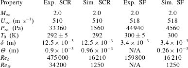
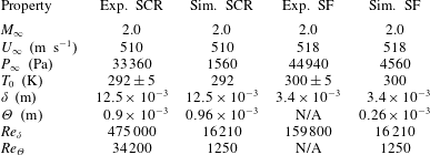
The flow conditions of the current work are described in table 1, in which the simulation conditions are placed in context with those of the experiments for both the SCR (Vanstone et al. Reference Vanstone, Saleem, Seckin and Clemens2016) and SF (Baldwin et al. Reference Baldwin, Arora, Kumar and Alvi2016; Arora et al. Reference Arora, Ali, Zhang and Alvi2018) configurations. The simulation Reynolds number  $(Re)$ is reduced for computational feasibility, while maintaining the free-stream Mach number
 $(M_{\infty })$ and velocity
 $(U_{\infty })$, the stagnation temperature
 $(T_{0})$ and the boundary-layer momentum
 $(\unicode[STIX]{x1D6E9})$ and outer-scale
 $(u(\unicode[STIX]{x1D6FF})=0.99U_{\infty })$ thicknesses, and reducing the free-stream pressure
 $(P_{\infty })$. This approach has proven successful for the proper reproduction of STBLI physics, including the analysis of unsteady features (Morgan et al. Reference Morgan, Duraisamy, Nguyen, Kawai and Lele2013; Adler & Gaitonde Reference Adler and Gaitonde2018a).
Experimental and computational flow conditions for SCR and SF STBLIs.
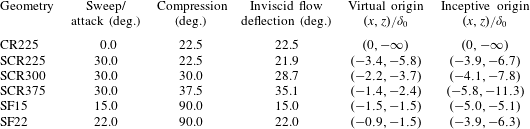
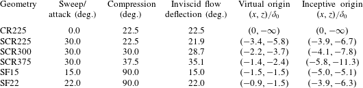
The parameter space of the interaction geometry considered is described in table 2. Two SF, three SCR, and one compression ramp with no sweep (CR) are studied. Details of several relevant angles and the locations of the VCO and inceptive conical origin (ICO) with respect to the geometric origin (the fin-tip/plate junction or the upstream-ramp-corner/side-boundary) are included. The virtual origin is the origin of conical symmetry, whereas the inceptive origin describes the effects of the incoming boundary-layer thickness on deviation from true conical symmetry; the two appear coincident with the geometric origin in the limit of radius  $(r)$ much larger than boundary-layer thickness
 $(\unicode[STIX]{x1D6FF})$. The dependence of the VCO and ICO position on interaction strength and mechanisms of interaction inception has recently been documented (Adler & Gaitonde Reference Adler and Gaitonde2019a).
Geometries of interest: angles of sweep/attack, compression and inviscid flow deflection, with corresponding displacement of simulation virtual and inceptive origins from geometric origin. Experimental comparison available for cases SCR225 and SF15. Inviscid shock detachment occurs at  ${\approx}23.0^{\circ }$ flow deflection.
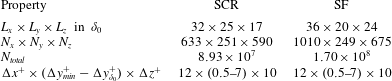
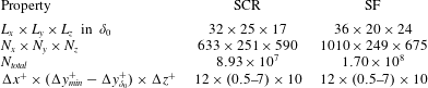
Details of the numerical discretization, boundary conditions and mean-flow validation for the current database are well documented in previous publications (Adler & Gaitonde Reference Adler and Gaitonde2017, Reference Adler and Gaitonde2018b; Adler et al. Reference Adler, Gonzalez, Stack and Gaitonde2018; Adler & Gaitonde Reference Adler and Gaitonde2019a) and will, therefore, be treated with brevity. The computational grids employed are described in table 3. They comprise  $8.9\times 10^{7}{-}1.7\times 10^{8}$ total points, with near wall resolution
 $(\unicode[STIX]{x0394}x^{+}\times (\unicode[STIX]{x0394}y_{min}^{+}-\unicode[STIX]{x0394}y_{\unicode[STIX]{x1D6FF}}^{+})\times \unicode[STIX]{x0394}z^{+})=(12\times (0.5{-}7)\times 10)$, in which the streamwise
 $(x)$, plate-normal
 $(y)$ and spanwise
 $(z)$ spacing are non-dimensionalized using boundary-layer inner variables (denoted with ‘
 $^{+}$’) (Smits & Dussauge Reference Smits and Dussauge2006). This resolution is sufficient for both the simulation of boundary-layer turbulence (Poggie et al. Reference Poggie, Bisek and Gosse2015) as well as STBLIs (Priebe & Martín Reference Priebe and Martín2012; Morgan et al. Reference Morgan, Duraisamy, Nguyen, Kawai and Lele2013). The span of the domain extends in excess of
 $17\unicode[STIX]{x1D6FF}$ for all simulations to facilitate examination of 3-D flow similarity. Synthetic turbulence (Adler et al. Reference Adler, Gonzalez, Stack and Gaitonde2018) is introduced on the inflow boundary,
 $18\unicode[STIX]{x1D6FF}$ upstream of the geometric origin, to allow for development of the incoming turbulent boundary layer. The plate, ramp and fin surfaces are modelled as adiabatic, no-slip walls. Adler & Gaitonde (Reference Adler and Gaitonde2019a) discuss the characteristic-based boundary treatment for the other boundaries. Various quantities have been validated in conjunction with experiments for both the SCR (Vanstone et al. Reference Vanstone, Saleem, Seckin and Clemens2016, Reference Vanstone, Musta, Seckin and Clemens2018) and SF (Baldwin et al. Reference Baldwin, Arora, Kumar and Alvi2016; Arora et al. Reference Arora, Ali, Zhang and Alvi2018) configurations. These include comparisons of surface flow visualization, surface pressure and all three velocity components in both Cartesian and spherical coordinates, which are discussed by Adler & Gaitonde (Reference Adler and Gaitonde2017, Reference Adler and Gaitonde2018b, Reference Adler and Gaitonde2019a).
Computational grid properties.
3 Flow structure
The flow fields associated with the SCR and SF interactions display key distinctions from their spanwise-homogeneous, 2-D counterparts. These have consequence on the unsteadiness, and are first summarized in this section to set the stage for the subsequent discussion.
3.1 Quasi-conical (3-D) symmetry of outer flow
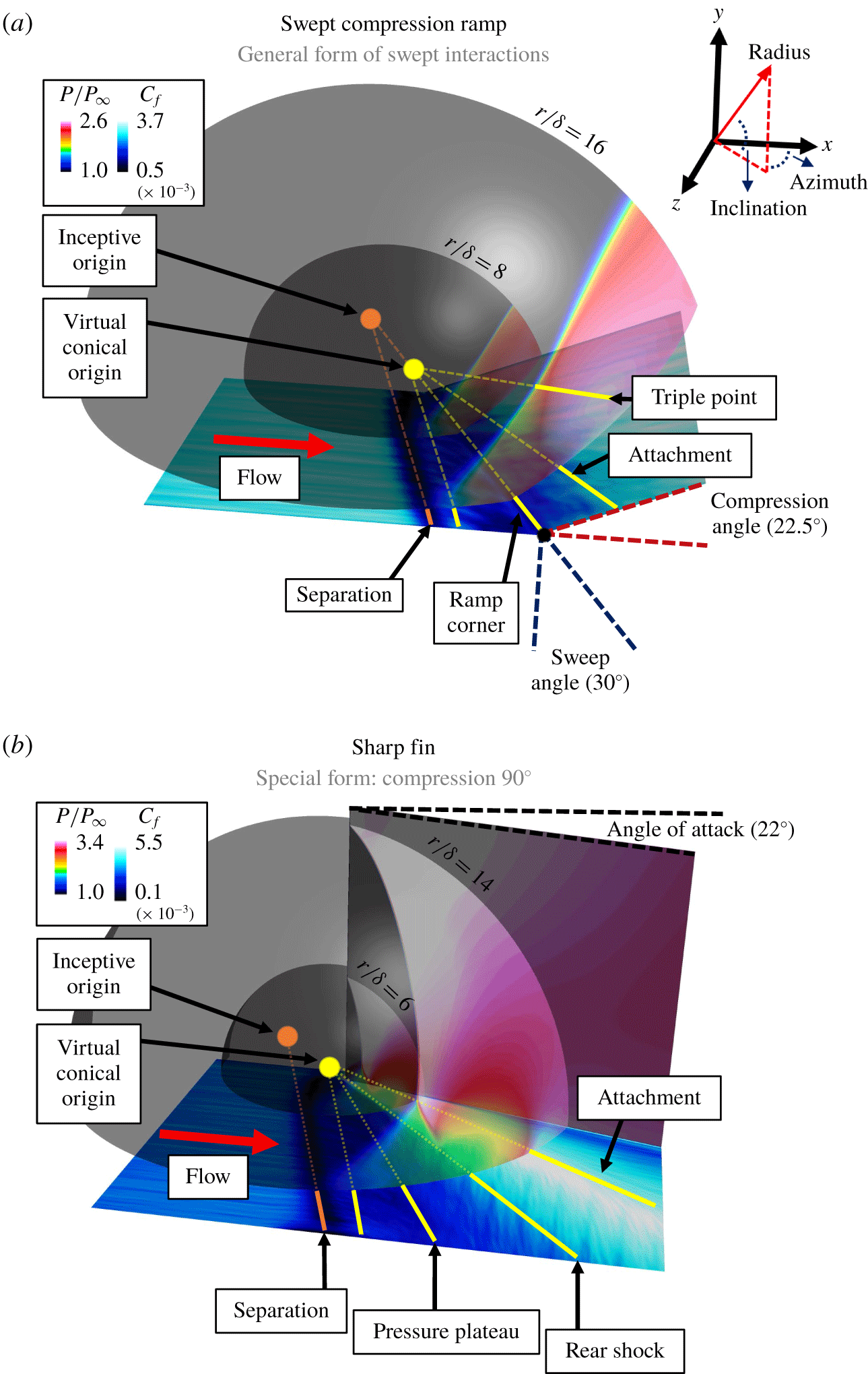
Illustration of quasi-conical (spherical) mean-flow symmetry for the SCR (a) and SF (b) interactions. Concentric spherical surfaces and the fin surface are coloured by pressure, whereas the plate and ramp surfaces are coloured by skin-friction coefficient magnitude. Lines emanating from the VCO demonstrate conformation of the interaction features to quasi-conical symmetry, with annotations of relevant flow features included.
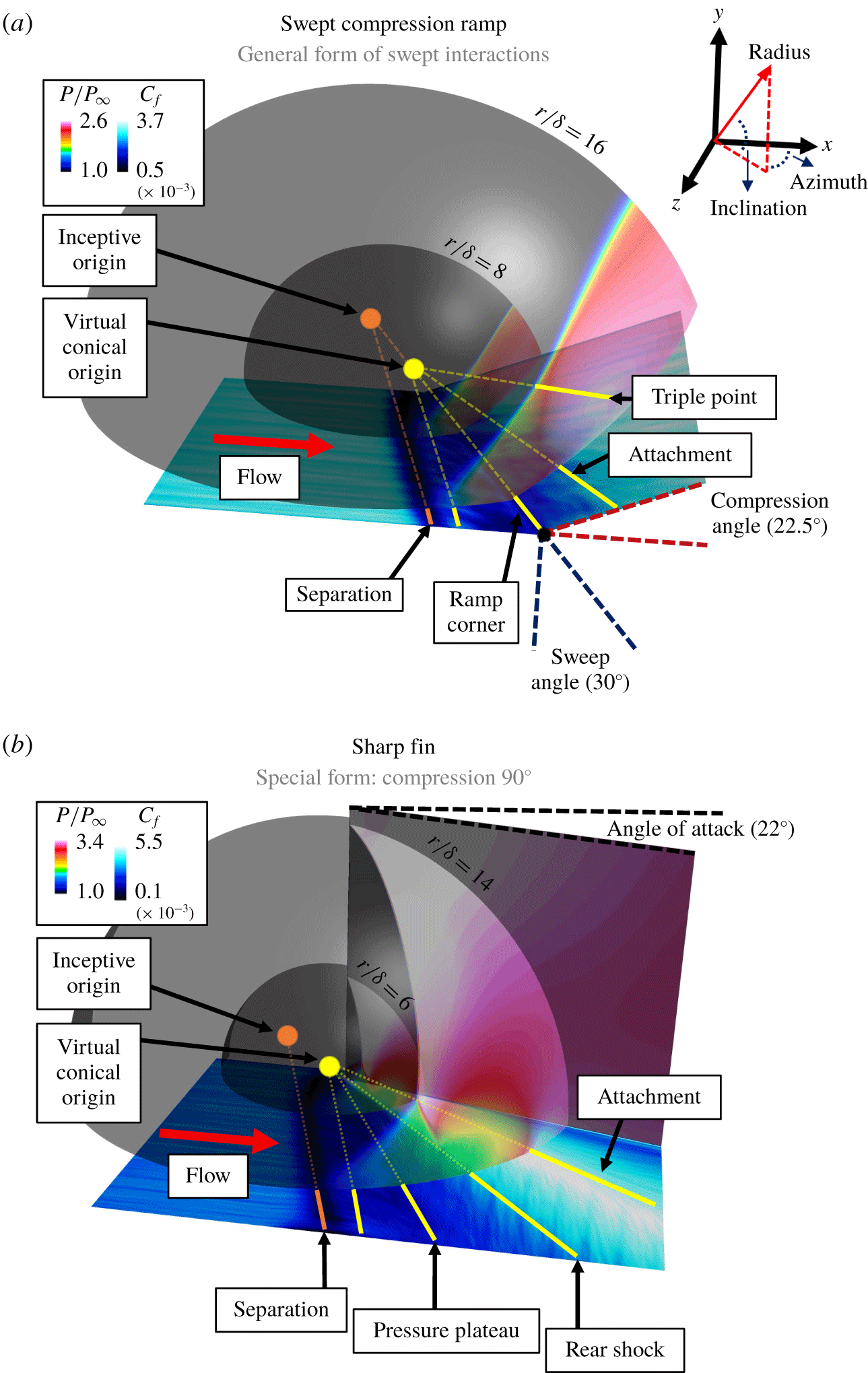
Perhaps the most significant distinctive feature of the 3-D STBLIs of interest is the common ‘quasi-conical’ symmetry exhibited by the time-mean outer flows. The description of ‘conical’ arises from observation that these interactions exhibit separation, attachment, and shock-triple-point lines that outline a conical structure; each of these lines emanates from the cone apex (the VCO) and extends indefinitely downstream and across the interaction span. The qualification ‘quasi-’ indicates that the conical symmetry is not perfect; it is mildly perturbed by the incoming boundary layer, which introduces a 2-D scale (the boundary-layer thickness) that is incompatible with 3-D perfect conical symmetry. Quantitatively, quasi-conical symmetry is best realized by observing the existence of similarity in the 3-D mean flows when viewed in spherical coordinates; this draws distinction from the spanwise-homogeneous (Cartesian) symmetry of 2-D STBLIs. Figure 2 displays the mean-flow symmetry and features of two representative 3-D STBLIs, including a SCR (a) and SF (b) interaction, respectively. The angles of sweep, compression and attack are marked, along with several mean-flow features, including the separation and attachment lines. Also marked are the VCO, as well as an inceptive origin, the significance of which has been discussed extensively by Adler (Reference Adler2019), and summarized below. Each figure shows mean pressure ( $p/p_{\infty }$) on two concentric (VCO-centred) spherical surfaces. These clearly display the common, cone-like, lambda-shock structure with apex at the VCO, indicating the conical growth of the outer flow with displacement from the VCO. The skin-friction coefficient magnitude,
 $C_{f}\geqslant 0$ is displayed on the plate and ramp surfaces to indicate the footprint of the quasi-conical outer flow on the plate surface. The location of flow separation is identified by the skin-friction magnitude tending toward zero; downstream of flow separation, the skin-friction magnitude increases above the upstream value, reflecting the strong flow separation and developed cross-flow exhibited by the interactions (Adler & Gaitonde Reference Adler and Gaitonde2019a). It is evident that the separation length (
 $L$: the arc-length between separation and attachment) grows linearly with displacement from the VCO, and unlike in the corresponding 2-D interactions, it is a local, not global, property of the flow.
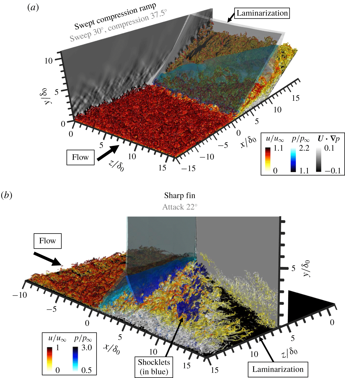
Three-dimensional renderings of representative flow instances for the SCR (a) and SF (b) interactions. Isosurfaces of the invariant Q-criterion (coloured by streamwise velocity) highlight hairpin vortices and the general flow structure. The shock (coloured by pressure in blue) and background shading are indicated by an isosurface and contours of  $\boldsymbol{U}\boldsymbol{\cdot }\unicode[STIX]{x1D735}p$.
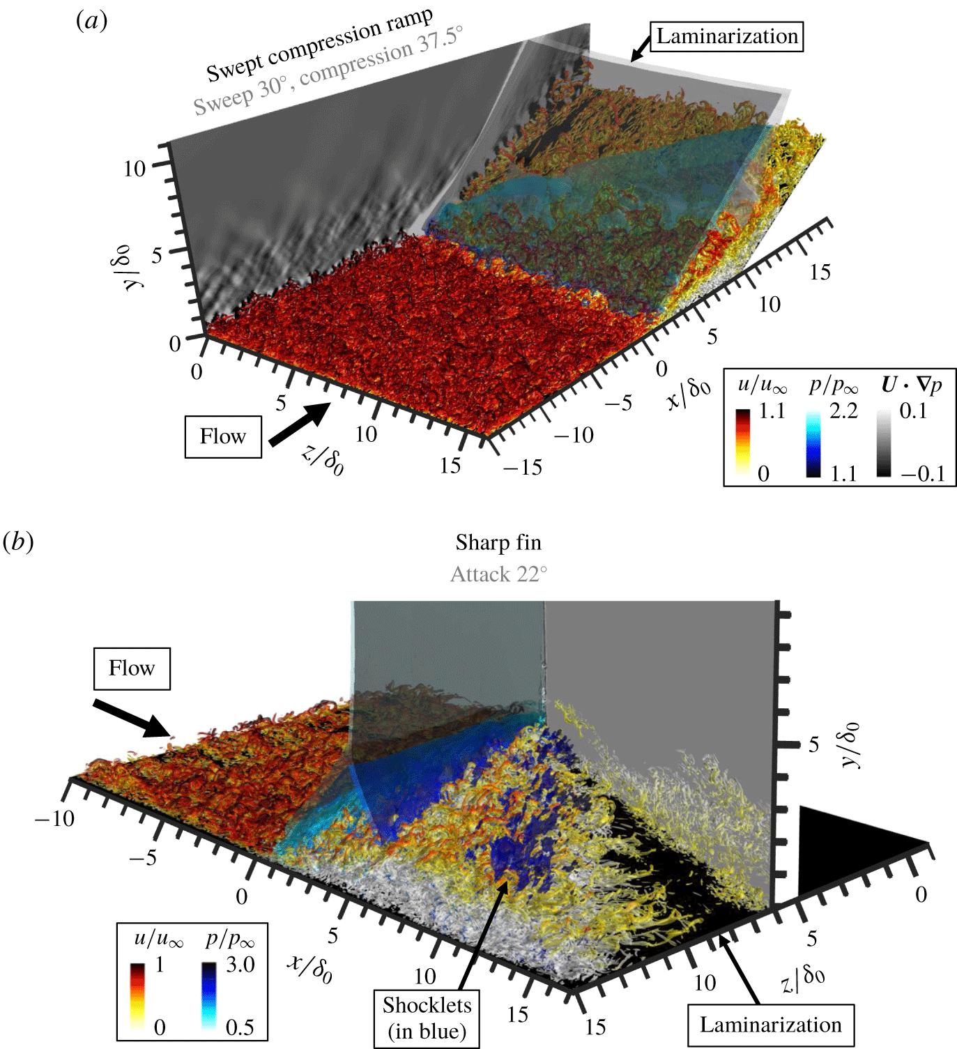
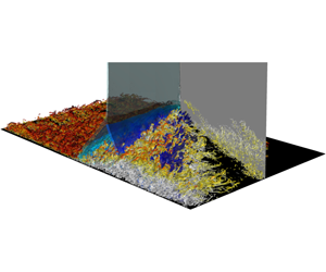
Representative instances of the flow are rendered in figure 3, in which the interaction of the turbulent boundary layer (red colour map) is visualized along with the shock structure (blue colour map), highlighting the large separation of scales between the shock structure and turbulent fluctuations. The structure of the turbulent boundary layer is visualized using an iso-surface of the Q-criterion (the second invariant of the velocity gradient tensor), effectively highlighting regions of large vorticity relative to strain rate. Many similarities are evident between the SCR and SF configurations, in both mean and instantaneous flow features, including the lambda-shock structure and outer flow, as well as the post-separation growth of the separated shear layer. Differences arise downstream of the main shock because attachment for the SCR interaction occurs on the shock generator (ramp) surface, whereas attachment for the SF interaction occurs on the plate surface; however, downstream of attachment, a significant reduction in turbulence kinetic energy occurs in both interactions due to similarities in the 3-D attachment process.
A notable distinction between these swept, 3-D interactions and comparably strong spanwise-homogeneous, 2-D interactions is the behaviour of the attaching flow. Strong 2-D interactions exhibit significant streamwise-reversed mean flow and strict flow recirculation, in which mean-flow streamlines retrace themselves. In contrast, the post-attachment ‘upstream’ propagating flow in 3-D interactions is not reversed relative to the free stream; rather, it assumes a strong cross-flow velocity component in the spanwise direction, resulting in a helical pseudo-recirculation vortex oriented away from the VCO. Consequently, the separation topology for swept, 3-D interactions remains unclosed as opposed to the closed separation topology of strong, 2-D interactions (Adler Reference Adler2019).
3.2 Competing 2-D and 3-D (free interaction) symmetry of inner shear flow
While the swept-shock generator introduces 3-D (conical) symmetry to the interaction, the incoming boundary layer (thickness  $\unicode[STIX]{x1D6FF}$) introduces 2-D (spanwise-homogeneous) symmetry to the interaction. These competing similarity scaling laws result in several flow phenomena that are more conveniently described in one symmetry than another, and many phenomena that must necessarily be described as a combination of both scaling laws. The addition of 2-D scaling to 3-D scaling leads to the distinction of ‘quasi-conical symmetry’ from ‘conical symmetry’ in the literature; the term quasi-conical reflects the presence of 2-D features in the otherwise perfectly 3-D conical flow. The quasi-conical description of the flow is also related to the concept of interaction inception, in which the local 2-D length scales become insignificant relative to the local 3-D length scales with increasing displacement from the VCO. For example, an approximately 2-D offset may be observed in figure 2 between the separation line (orange: emanating from the inceptive origin) and the farthest upstream line emanating from the VCO (yellow) – this offset becomes small relative to the local separation length moving away from the VCO. The prominent inceptive effects appear to be well described in the region of flow separation by the inceptive origin concept (Adler & Gaitonde Reference Adler and Gaitonde2019a).
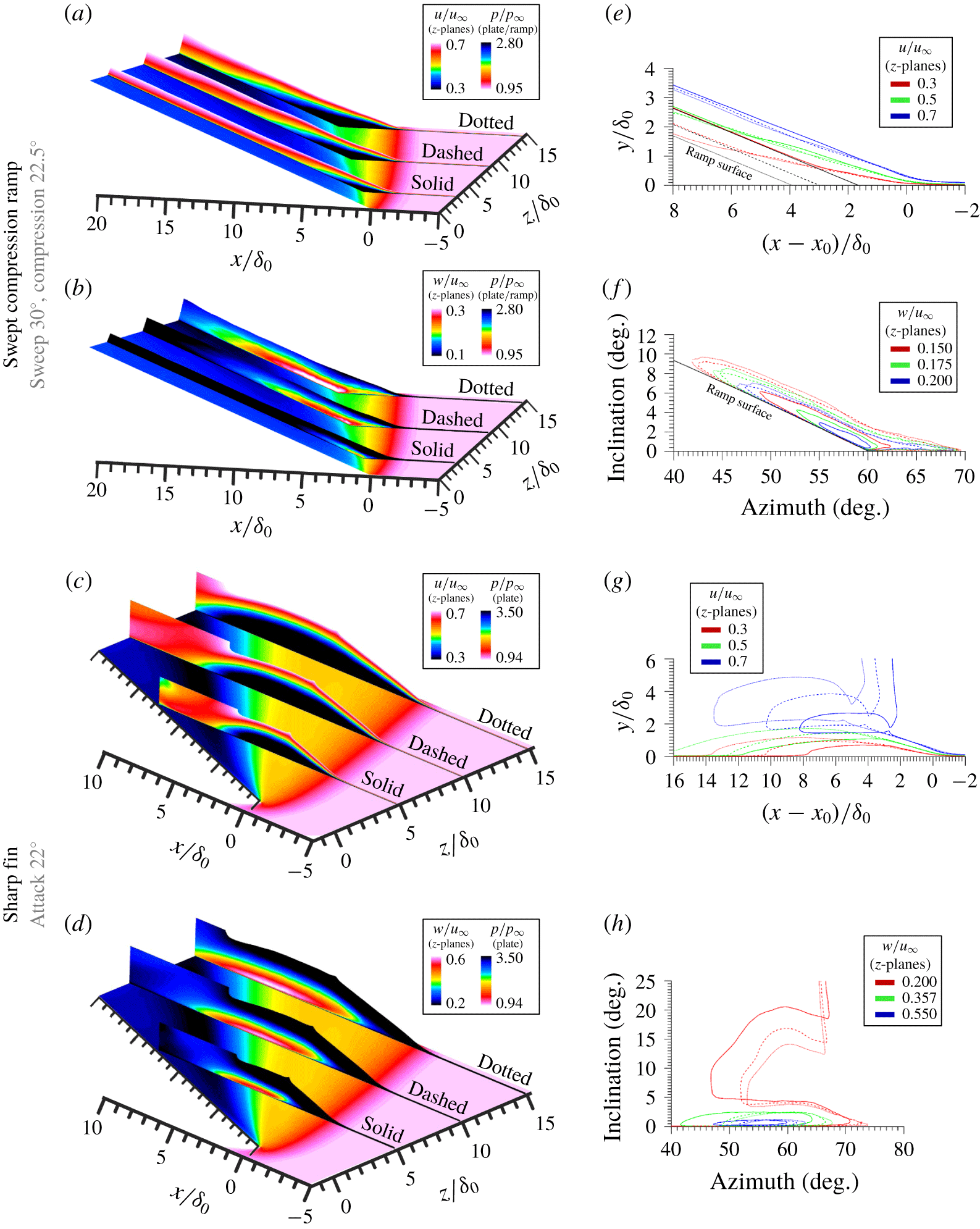
Demonstration of competing 2-D and 3-D scaling laws in swept STBLIs evident in mean profiles of the inner (cross-flow) and outer (main) shear layers at successive spanwise stations. (a,b,e,f) SCR,  $30^{\circ }$ sweep,
 $22.5^{\circ }$ compression. (c,d,g,h) SF,
 $22^{\circ }$ attack. (a–d) Walls coloured by pressure. (a,c)
 $z$-planes coloured by streamwise velocity. (b,d)
 $z$-planes coloured by spanwise velocity. (e,g) Streamwise velocity contours from
 $z$-planes of (a,c); streamwise spatial coordinate aligned at local separation location. (f,h) Spanwise velocity contours from
 $z$-planes of (b,d) in spherical VCO-centred coordinates.
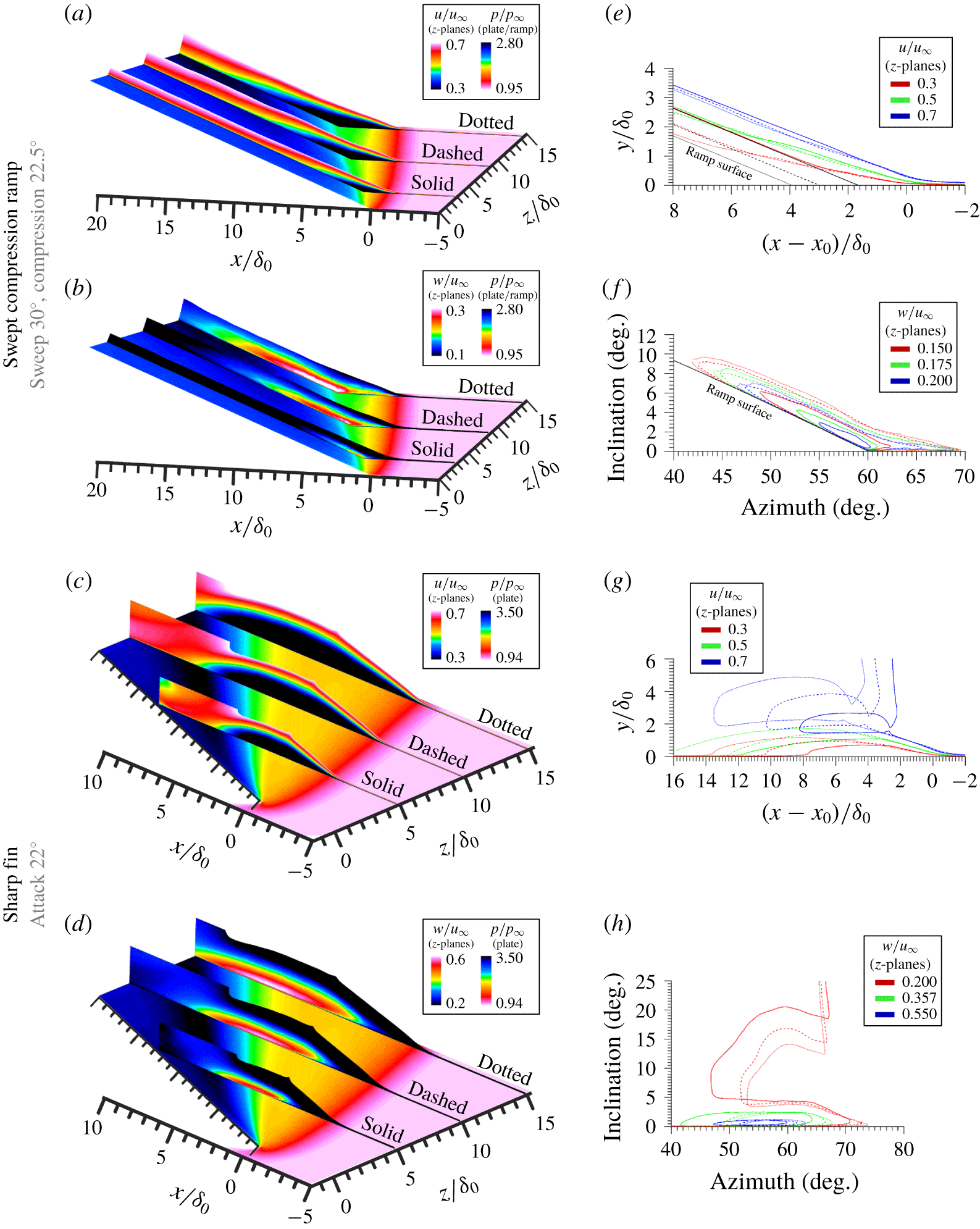
To understand the full ramifications of these competing 2-D and 3-D scaling laws, figure 4 isolates the symmetry type of several on-plate and off-plate flow features in the inner (b,d,f,h) and outer (a,c,e,g) shear layers, along with a quantitative demonstration of mean-flow profile collapse in the representative Cartesian (e,g) or spherical (f,h) coordinate system (e–h), for both the SCR (a,b,e,f) and SF (c,d,g,h) STBLIs. The plate surface is coloured by mean pressure, reflecting the quasi-conical footprint of the interaction, whereas the outer (main) shear layer is isolated by  $z$-plane contours of mean streamwise velocity (a,c) at several spanwise stations, and the inner (cross-flow) shear layer is isolated by
 $z$-plane contours of mean spanwise velocity (b,d) at several spanwise stations. For both configurations, these results demonstrate excellent collapse of the outer (main) shear layer in Cartesian coordinates, reflecting the underlying 2-D symmetry (offset for local separation location); this supports the claim of classical (2-D) free-interaction theory of Chapman et al. (Reference Chapman, Kuehn and Larson1957), in that the mean-flow profiles in the vicinity of separation are independent of the downstream obstacle (which is enlarging in the spanwise direction). Additionally, these results demonstrate excellent collapse of the inner (cross-flow) shear layer in VCO-centred spherical coordinates for spanwise stations sufficiently far from the geometric origin (excluding the first station), beyond which inceptive effects are negligible. This reflects the underlying 3-D (quasi-conical) symmetry, and supports the claim of conical (3-D) free-interaction theory of Settles & Kimmel (Reference Settles and Kimmel1986), in that, for given upstream conditions and swept-shock geometry, the mean-flow profiles in the quasi-conical interaction region exhibit collapse in spherical (VCO-centred) coordinates.
Interestingly, 3-D scaling is exhibited by the pseudo-inviscid outer flow as well as the viscous, inner (cross-flow), shear layer. However, between these two layers, 2-D scaling is prominent in the viscous, outer (main), shear layer, not only in the vicinity of separation, but also throughout the interaction and near attachment. That is, the outermost pseudo-inviscid footprint of the interaction and the innermost viscous shear layer exhibit quasi-conical symmetry, whereas the middle, viscous, shear layer exhibits spanwise-homogeneous symmetry, fed from the incoming boundary layer. The ramifications of these scaling behaviours on both the mid-frequency unsteadiness (shear layer coherence) and high-frequency unsteadiness (integral scale fluctuations) are examined in § 4.
It should be noted that none of the strong, swept, 3-D interactions of the current database exhibit secondary separation (Panaras Reference Panaras1996), likely precluded by the relatively small Mach number. Schmisseur & Gaitonde (Reference Schmisseur and Gaitonde2001) discuss the genesis of secondary separation in the context of both swept and crossing shock interactions. The presence of secondary separation would introduce additional complications to this discussion of mean-flow scaling and is worthy of follow-on investigation.
4 Unsteadiness
4.1 Wall-pressure spectra
4.1.1 Differences between 2-D and 3-D interactions
The unsteady dynamics of spanwise-homogeneous, 2-D STBLIs has been thoroughly investigated for both the impinging-oblique-shock (Dupont et al. Reference Dupont, Haddad and Debiève2006; Touber & Sandham Reference Touber and Sandham2009; Agostini et al. Reference Agostini, Larcheveque, Dupont, Denieve and Dussauge2012; Aubard et al. Reference Aubard, Gloerfelt and Robinet2013; Adler & Gaitonde Reference Adler and Gaitonde2018a) and compression-ramp (Ganapathisubramani et al. Reference Ganapathisubramani, Clemens and Dolling2009; Priebe & Martín Reference Priebe and Martín2012) configurations. Relevant time scales  $(\unicode[STIX]{x1D70F}=1/St_{\unicode[STIX]{x1D6FF}})$ for prominent mid-frequency and low-frequency unsteadiness in these spanwise-homogeneous STBLI range from
 $\unicode[STIX]{x1D70F}\sim O(10)$ for Kelvin–Helmholtz phenomena induced within the separated shear layer, to
 $\unicode[STIX]{x1D70F}\sim O(300)$ for low-frequency bubble breathing, while the dominant frequencies of the incoming turbulent boundary layer are of higher frequency and coincide with the boundary-layer characteristic time,
 $\unicode[STIX]{x1D70F}\gtrsim O(1)$ (Agostini et al. Reference Agostini, Larcheveque, Dupont, Denieve and Dussauge2012; Adler & Gaitonde Reference Adler and Gaitonde2018a). The low-frequency unsteadiness appears to scale well with the size of the separation (Dupont et al. Reference Dupont, Haddad and Debiève2006; Dussauge et al. Reference Dussauge, Dupont and Debiève2006) and generally collapses with Strouhal number (
 $St_{L}=fL/U_{\infty }$) based on the nominal length of the separation bubble,
 $L$.
The unsteady dynamics of spanwise-non-homogeneous, swept, 3-D, interactions is distinctly different. In these configurations the separation length,  $L$, increases across the span with displacement from the VCO, and indeed, we observe
 $St_{\unicode[STIX]{x1D6FF}}$, not
 $St_{L}$, to be the most appropriate primary non-dimensionalization for unsteadiness in these interactions, which conspicuously lack the prominent low-frequency (
 $St_{L}\sim 0.03$,
 $St_{\unicode[STIX]{x1D6FF}}\sim 0.006$) band of unsteadiness (two decades below the prominent boundary-layer frequencies) found in spanwise-homogeneous interactions. The unsteady features of the SF STBLIs have many similarities to those of the SCR STBLIs in the high-, mid- and low-frequency bands, indicating that the dynamics of 3-D interactions is distinctly different than 2-D interactions, and suggesting that 3-D interactions exhibit commonality of unsteady features for a wide variety of configurations.
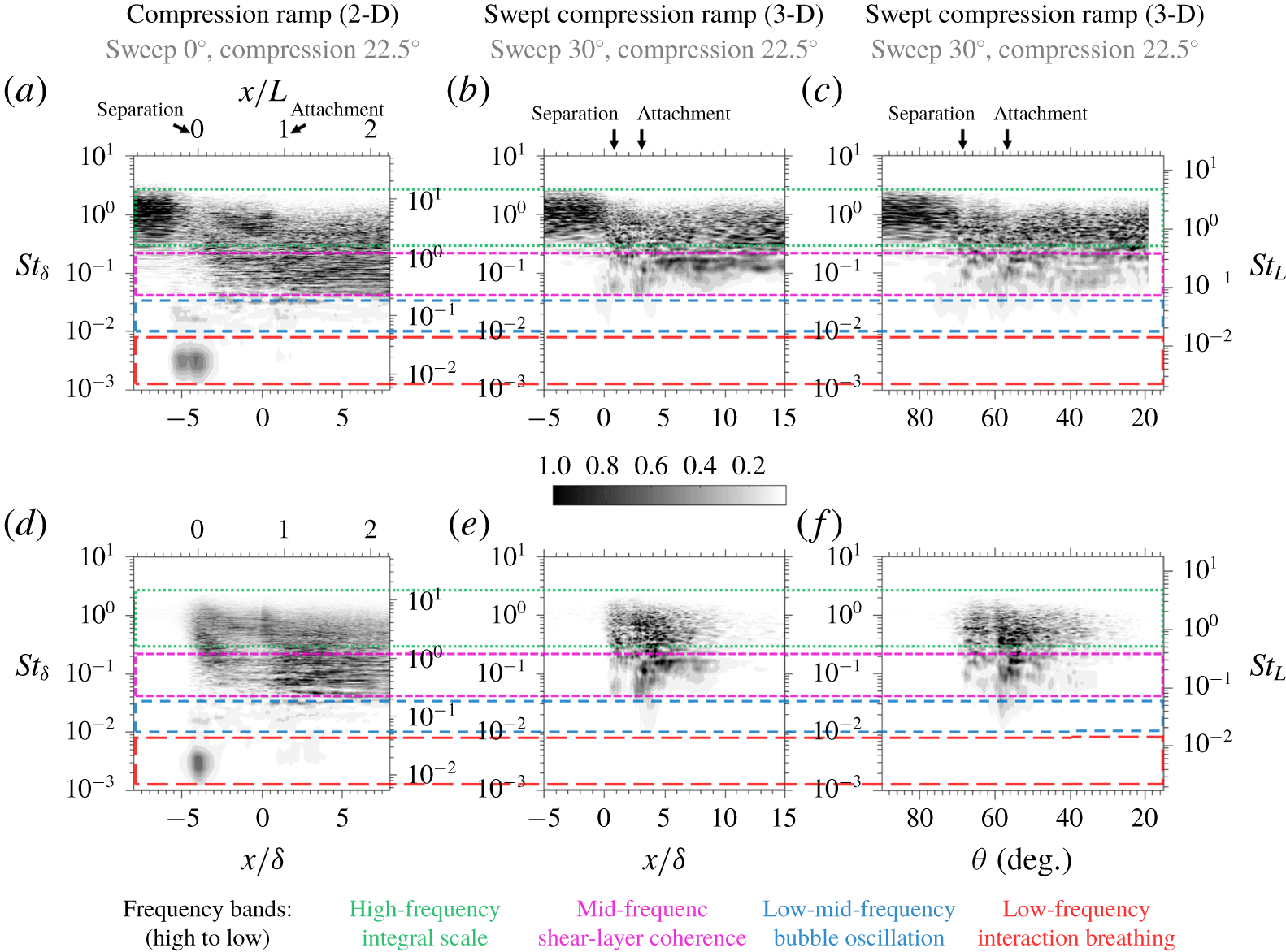
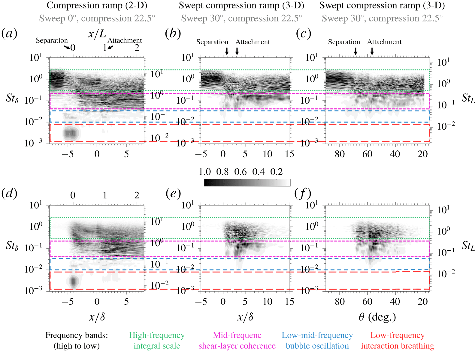
Comparison of premultiplied  $(St\times PSD(St))$, wall-pressure PSD between (a,d) 2-D unswept-compression-ramp (sweep
 $0^{\circ }$, compression
 $22.5^{\circ }$) and (b,c,e,f) 3-D SCR (sweep
 $30^{\circ }$, compression
 $22.5^{\circ }$). Spatial location (horizontal axis) represented by Cartesian (
 $z/\unicode[STIX]{x1D6FF}=10$;
 $x/\unicode[STIX]{x1D6FF}$ free: a,b,d,e) and spherical (
 $r/\unicode[STIX]{x1D6FF}=10$;
 $\unicode[STIX]{x1D703}$ free: c,f) coordinates. PSD are normalized locally in (a–c) and globally in (d–f). Non-dimensional frequency (vertical axis) formed using boundary-layer thickness (
 $St_{\unicode[STIX]{x1D6FF}}$: left vertical) and local separation length (
 $St_{L}$: right vertical). Annotations demarcate the high-frequency integral-scale band (
 $\cdots \cdots$), mid-frequency shear-layer-coherence band (– – – –, violet), low-mid-frequency bubble-oscillation band (– – –, blue), and low-frequency interaction-breathing band (– –). Notably, the prominent low-frequency unsteadiness in the 2-D, spanwise-homogeneous interaction is suppressed in the 3-D, swept interaction.
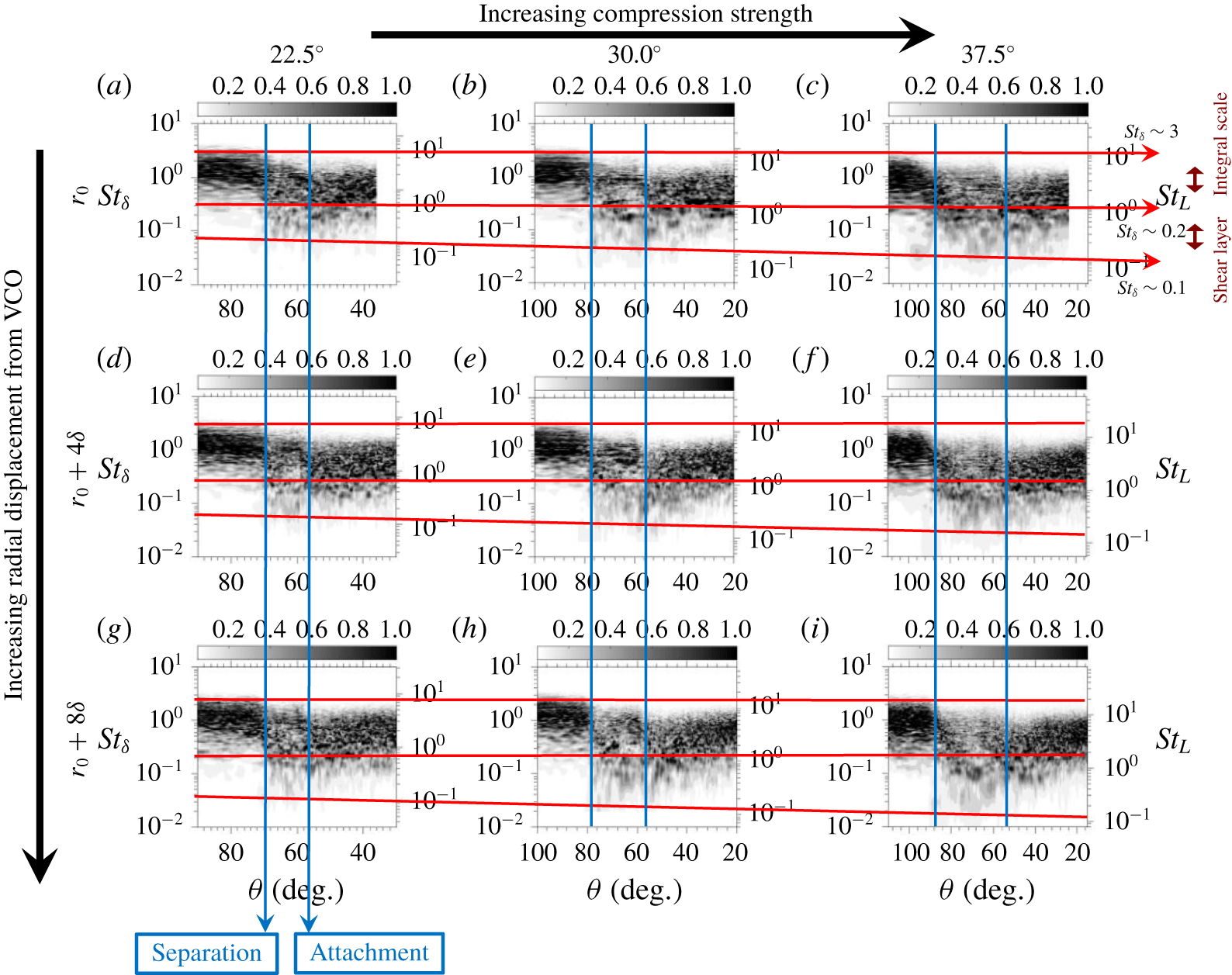
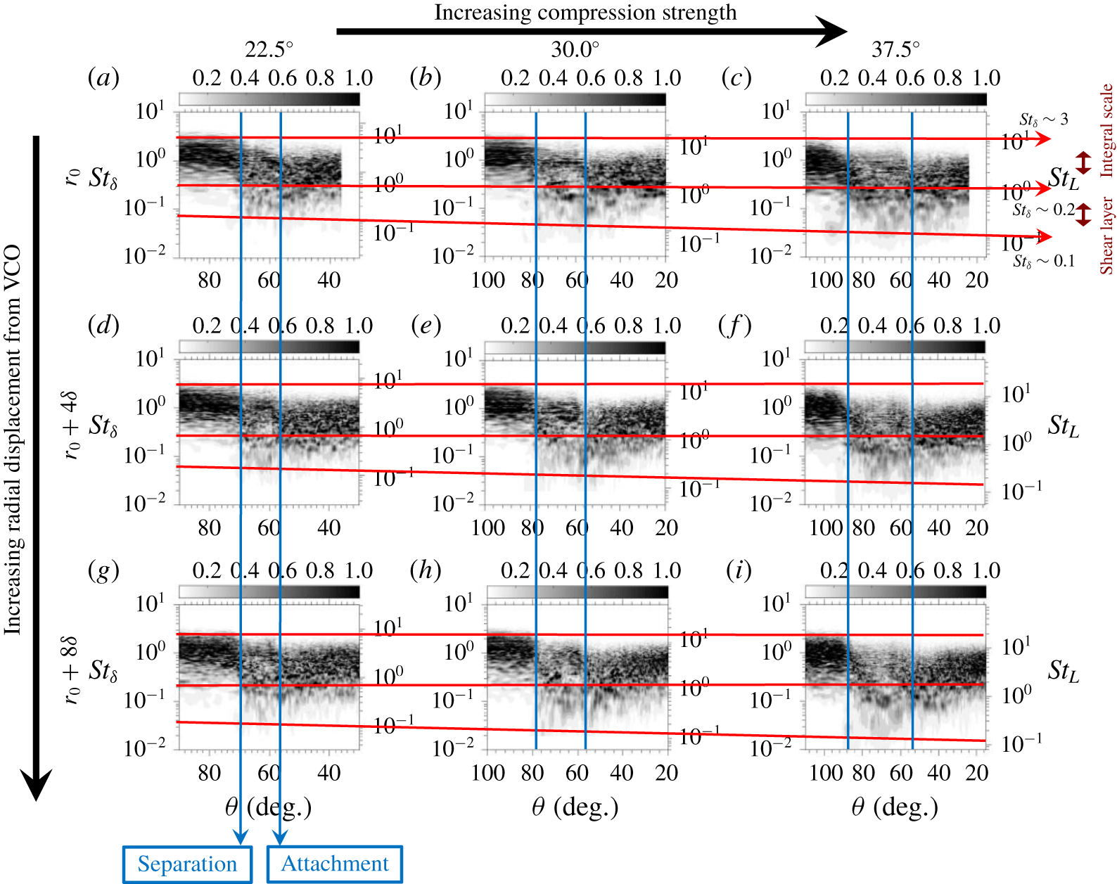
SCR: premultiplied and normalized fluctuating wall-pressure PSD as a function of azimuthal angle (horizontal). Frequency is described by boundary-layer Strouhal number ( $St_{\unicode[STIX]{x1D6FF}}$: left vertical) and local separation arc-length Strouhal number (
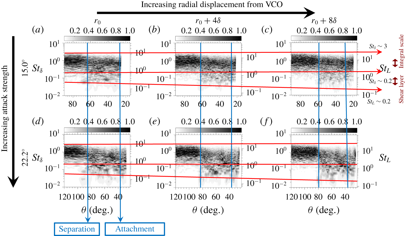
 $St_{L}$: right vertical). The PSD matrix is organized via increasing compression strength left-to-right across the rows and increasing radial displacement from the VCO top-to-bottom down the columns to demonstrate the spatial collapse of the spectra in the conical frame (parallel blue lines) and the lowering of the mid-frequency band of unsteadiness with increasing interaction strength (downward sloping red lines).
These considerations are now discussed quantitatively, with various figures describing the wall-pressure power-spectral-density (PSD) dependence on streamwise coordinate  $(X/\unicode[STIX]{x1D6FF})$ or azimuthal angle
 $(\unicode[STIX]{x1D703})$ for each of the geometries described in table 2. The azimuthal angle (see schematic in figure 2) describes the angle (in the plane of the incoming boundary-layer wall and with vertex at the VCO) between the streamwise direction and the point of interest. Results for the unswept compression ramp are shown in figure 5(a,d), for the SCR in figures 5(b,c,e,f), 6 and 7 and for the SF in figures 8 and 9. Each will be discussed in context below. The ramp corner is located at
 $\unicode[STIX]{x1D703}=60^{\circ }$ for the SCR interactions. For both swept configuration types, large azimuthal angle corresponds to upstream displacement, whereas small azimuthal angle corresponds to downstream displacement. Except for figure 5(d–f), the PSD at each spatial location has been normalized such that the integral of premultiplied power over all resolvable frequencies is unity. In all cases, the PSD is obtained using Welch’s windowed overlapping segments estimator method by splitting the signal into 8 segments with 50 % overlap using Hamming windows. The PSD is premultiplied by the corresponding Strouhal number based on the mean incoming boundary-layer thickness to represent the power distribution effectively on a logarithmic scale. Each simulation is integrated in time in excess of
 $1500\unicode[STIX]{x1D6FF}/U_{\infty }$, with temporal data resolution of
 $0.05\unicode[STIX]{x1D6FF}/U_{\infty }$. This facilitates the reproduction of the known low-frequency band in 2-D interactions, with convergence of the spectra over more than 10 low-frequency cycles. In figures 6–9, spectra obtained for different interaction strengths and at different radii from the VCO are presented in a matrix, with annotative lines to illustrate various scaling laws for the fluctuation spectra.
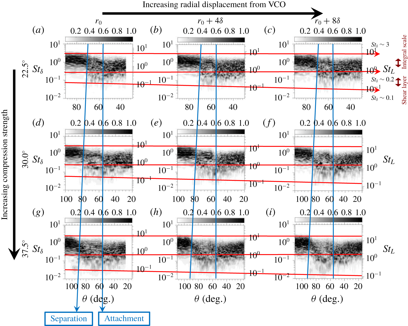
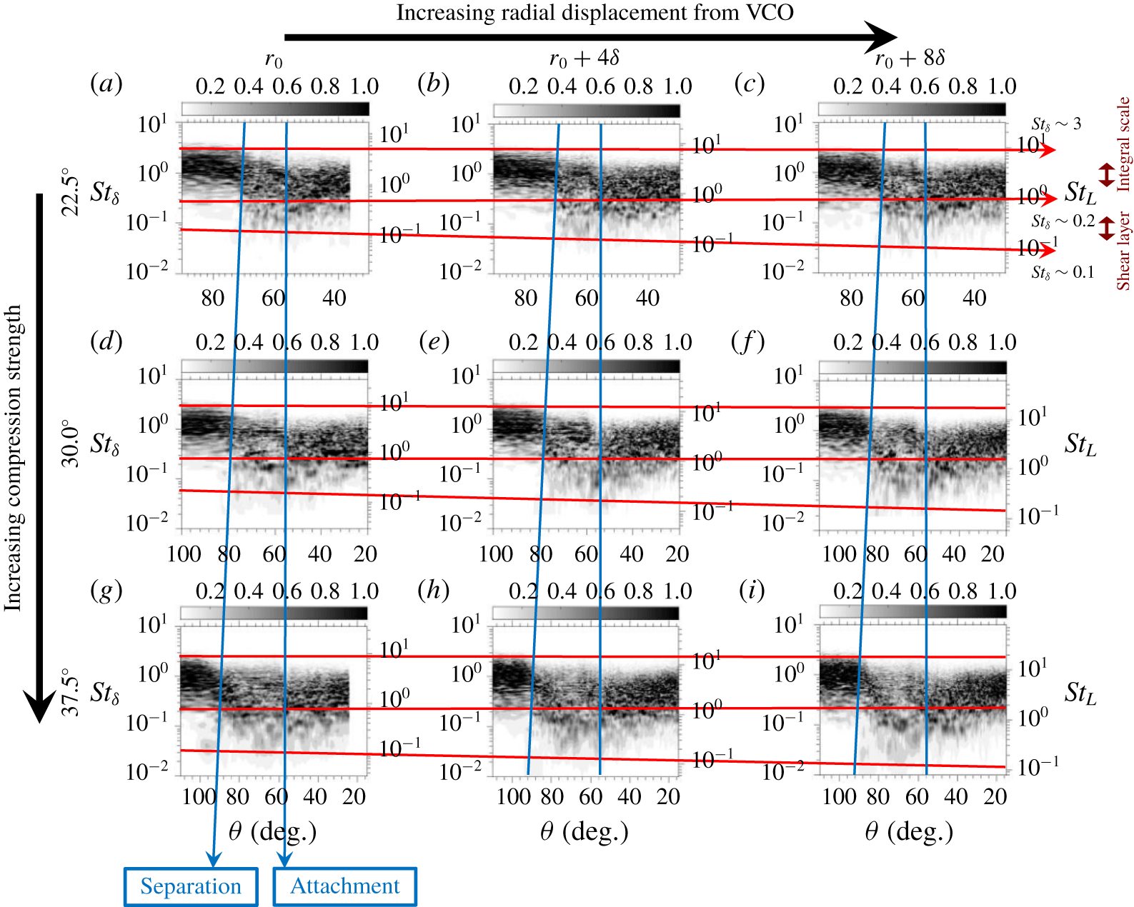
SCR: premultiplied and normalized fluctuating wall-pressure PSD as a function of azimuthal angle (horizontal). Frequency is described by boundary-layer Strouhal number ( $St_{\unicode[STIX]{x1D6FF}}$: left vertical) and local separation arc-length Strouhal number (
 $St_{L}$: right vertical). The PSD matrix is organized via increasing radial displacement from the VCO left to right across the rows and increasing compression strength top to bottom down the columns to demonstrate the competing 2-D scaling (horizontal red lines) and 3-D scaling (downward sloping read lines) for the mid-frequency unsteadiness. Additionally, the increase of interaction spreading rate with interaction strength is demonstrated by the non-parallel blue lines.
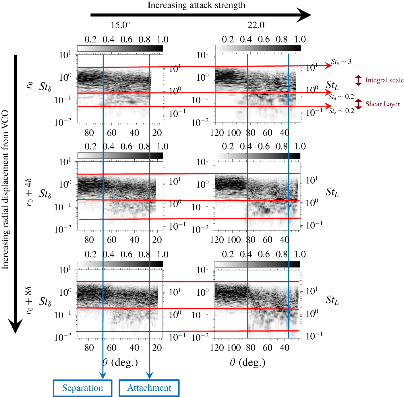
SF: premultiplied and normalized fluctuating wall-pressure PSD as a function of azimuthal angle (horizontal). Frequency is described by boundary-layer Strouhal number ( $St_{\unicode[STIX]{x1D6FF}}$: left vertical) and local separation arc-length Strouhal number (
 $St_{L}$: right vertical). The PSD matrix is organized via increasing compression strength left to right across the rows and increasing radial displacement from the VCO top to bottom down the columns to demonstrate the spatial collapse of the spectra in the conical frame (parallel blue lines) and the lowering of the mid-frequency band of unsteadiness with increasing interaction strength (downward sloping red lines).
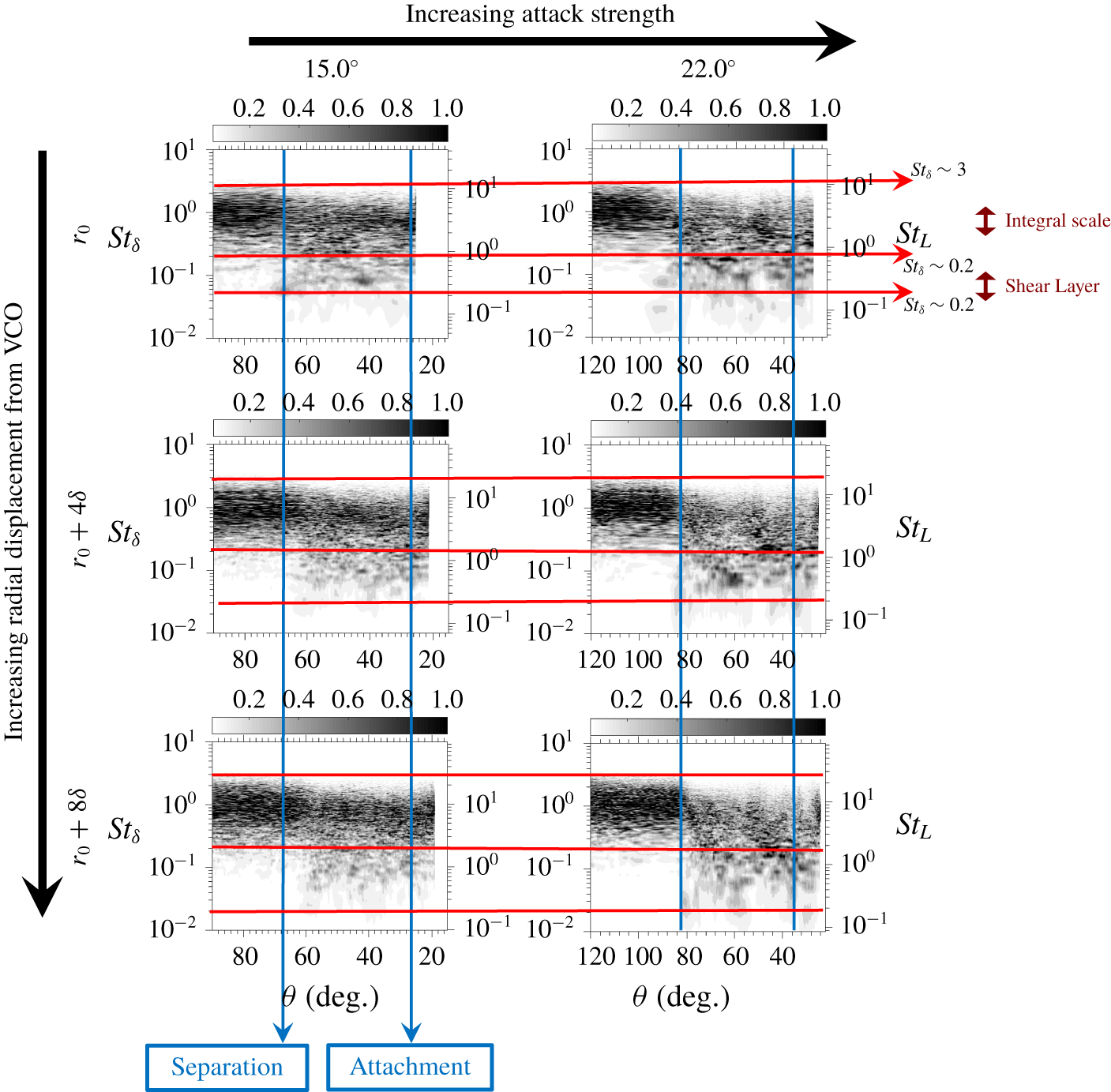
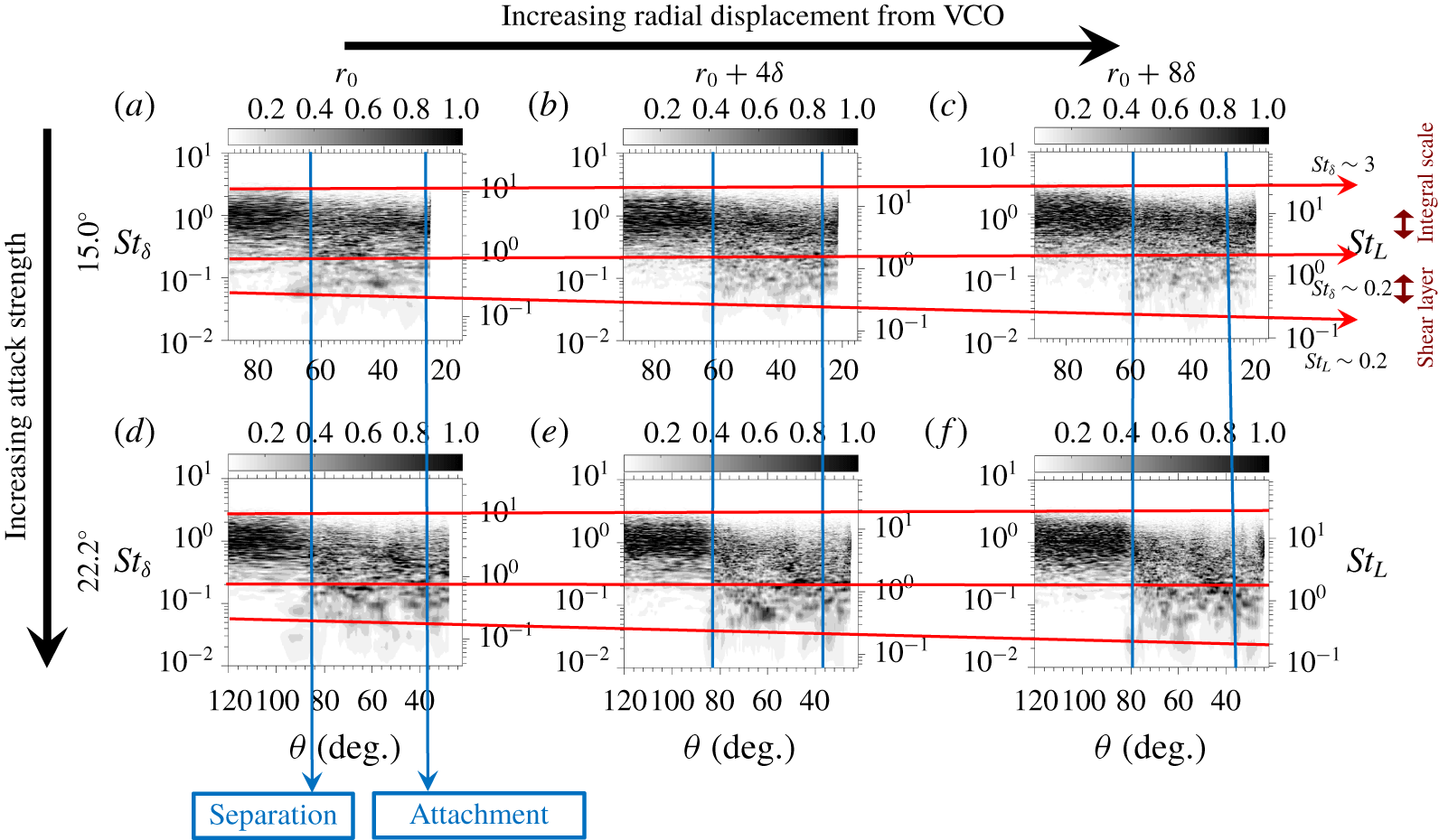
SF: premultiplied and normalized fluctuating wall-pressure PSD as a function of azimuthal angle (horizontal). Frequency is described by boundary-layer Strouhal number ( $St_{\unicode[STIX]{x1D6FF}}$: left vertical) and local separation arc-length Strouhal number (
 $St_{L}$: right vertical). The PSD matrix is organized via increasing radial displacement from the VCO left to right across the rows and increasing compression strength top to bottom down the columns to demonstrate the competing 2-D scaling (horizontal red lines) and 3-D scaling (downward sloping read lines) for the mid-frequency unsteadiness. Additionally, the increase of interaction spreading rate with interaction strength is demonstrated by the non-parallel blue lines.
Spectral comparison between the 2-D, unswept compression ramp and 3-D, SCR is presented in figure 5, along with annotation of the frequency bands relevant to 2-D STBLIs as described by Adler & Gaitonde (Reference Adler and Gaitonde2018a). Prominent low-frequency unsteadiness (two decades lower than the frequencies associated with the incoming turbulent boundary layer) is absent from the spectra of this SCR and all, swept, 3-D interactions of the present database. Notably, the comparison between the 2-D compression-ramp interaction (a) and the 3-D SCR interaction (b,c) differs only as a result of the introduction of sweep. The upstream flow conditions, numerical schemes and duration of temporal integration are maintained; this demonstrates that the 3-D interaction exhibits a suppressed low-frequency band relative to the 2-D interaction. This finding is consistent with the experimental observations of Gibson & Dolling (Reference Gibson and Dolling1991) as well as Schmisseur & Dolling (Reference Schmisseur and Dolling1992, Reference Schmisseur and Dolling1994), for the SF, along with Erengil & Dolling (Reference Erengil and Dolling1993), for the SCR. These studies identify the lowest significant unsteadiness in the swept interactions in a band only one decade below the characteristic boundary-layer frequencies. We classify this unsteadiness as mid-frequency unsteadiness rather than low-frequency unsteadiness, because it is largely associated with convective coherent structures formed in the separated shear layer (see § 4.2), not stationary large-scale (‘breathing’) unsteadiness of the separated region as a whole; necessarily, its mechanism is more similar to mid-frequency unsteadiness in comparable spanwise-homogeneous interactions, rather than the low-frequency unsteadiness in such interactions. Recent experiments also confirm this observation that the prominence of the mid-frequency fluctuation band is increased relative to the that of the low-frequency fluctuation band in swept interactions (Arora, Mears & Alvi Reference Arora, Mears and Alvi2019; Vanstone & Clemens Reference Vanstone and Clemens2019). We note that, by an absolute measure, the mid-frequency content in swept interactions may comprise lower or higher frequencies than the corresponding content in 2-D interactions, because the actual frequency depends on the local length and velocity scales. Relative to the mid-frequency band, these results indicate that swept interactions suppress a mechanism responsible for a still lower frequency band that would be present in the absence of sweep.
In contrast, the frequency characteristics of the high- and mid-frequency bands translate relatively well from the 2-D to 3-D interactions. The high-frequency band lowers in frequency moving through the interaction with decreasing local  $U/\unicode[STIX]{x1D6FF}$. The mid-frequency band becomes prominent after separation and persists throughout the interaction, relatively independent of the azimuthal coordinate.
For the present discussion, there is little need to distinguish between the subtle differences in the 3-D spectra resulting from the use of the Cartesian surface (b,e) or spherical surface (c,f) on which the spatial dependence (horizontal axis) of the surface pressure spectra are plotted; however, use of the spherical surface more appropriately reflects the mean-flow symmetry, and captures the mid-frequency band more consistently, especially for small azimuthal angle (large streamwise coordinate). A notable distinction arises between the amplitude behaviour of the high- and mid-frequency bands of the 2-D and 3-D interactions. For both bands, the amplitude of the downstream (small azimuth) fluctuations decays more rapidly for the swept interaction than the unswept interaction, due to the positive spanwise velocity component downstream of the interaction in the swept configuration.
4.1.2 Spectral trends in 3-D interactions
As discussed in § 3.2, the post-separation mean flow of swept STBLIs exhibits regions of shear with both 2-D and 3-D similarity scaling laws. This section demonstrates the influence of these competing scaling laws on the manner in which high-frequency upstream fluctuations are processed by the interaction, and particularly, the development of mid-frequency fluctuations within the interaction. Specifically, it is observed that the high-frequency fluctuations (integral-scale turbulence,  $St_{\unicode[STIX]{x1D6FF}}=0.2\lesssim f\lesssim St_{\unicode[STIX]{x1D6FF}}=3$, with non-dimensional frequency
 $f$) retain the 2-D scaling from the upstream boundary layer throughout the interaction; i.e. the development of high-frequency fluctuations with 3-D scaling within the interaction does not have adequate time for growth to overtake (in amplitude) the incoming 2-D scaling high-frequency fluctuations. However, the mid-frequency fluctuations (coherent shear-layer turbulence,
 $St_{L}=0.1\lesssim f\lesssim St_{\unicode[STIX]{x1D6FF}}=0.2$) exhibit aspects of 2-D and 3-D scaling at the upper and lower bounds of the mid-frequency band, respectively; i.e. the developing mid-frequency fluctuations with 3-D scaling within the interaction do indeed display adequate growth characteristics to compare with the amplitude of the developing 2-D-scaling mid-frequency fluctuations. Several quantitative demonstrations of the variability of 2-D versus 3-D mid-frequency scaling as a function of radial coordinate, interaction strength and interaction type follow.
The relationship of the wall-pressure PSD spatial signature to the interaction strength and radial displacement from the VCO is described in figures 6 and 7 for the SCR interactions followed by figures 8 and 9 for the SF interactions. The plots of figures 6 (SCR) and 8 (SF) are arranged in a matrix by increasing interaction strength from left to right across the rows and increasing radius from the VCO from top to bottom down the columns. Several lines crossing different panels are displayed to illustrate the principal observations. The blue lines facilitate comparison of the spatial scaling of the surface fluctuations for different radii. The parallel vertical nature of the blue lines reflects the near perfect (spatial) collapse of the wall-pressure fluctuation spectra in spherical coordinates for each interaction. A similar observation may be made regarding the red lines, which facilitate comparison of the frequency scaling of the surface fluctuations for different interaction strengths. When these are perfectly horizontal, the phenomenon exhibits 2-D frequency scaling with Strouhal number based on the incoming boundary-layer thickness ( $St_{\unicode[STIX]{x1D6FF}}$ on the left axis), independent of the interaction strength. The Strouhal number scaling based on the local separation arc length is designated with
 $St_{L}$ on the right axis: diverging (downward sloping) red lines reflect the thickening of the separated shear layer and stronger 3-D scaling (scaling with
 $St_{L}$) of mid-frequency fluctuations with increasing interaction strength.
Conversely, the plots of figures 7 (SCR) and 9 (SF) are arranged in a matrix by increasing radius from the VCO from left to right across the rows and increasing interaction strength from top to bottom down the columns. In this case, the blue lines facilitate comparison of the spatial scaling of the surface fluctuations for different interaction strengths. The diverging blue lines reflect the increase in interaction spreading rate with increasing interaction strength; that is, the arc length between separation and attachment grows more rapidly with increasing radius for stronger interactions. In this case, the red lines facilitate comparison of the frequency scaling of the surface fluctuations for different radii. Horizontal alignment reflects 2-D frequency scaling (scaling with  $St_{\unicode[STIX]{x1D6FF}}$ on the left axis), which is especially applicable for the high-frequency surface fluctuations. With Strouhal number based on the local separation arc-length (
 $St_{L}$) on the right axis, the diverging red lines thus reflect the competing 2-D (horizontal with constant
 $St_{\unicode[STIX]{x1D6FF}}$) and 3-D (downward sloping with constant
 $St_{L}$) scaling exhibited by the mid-frequency fluctuations.
In all of the spectra, high frequencies typical of integral scale features of the incoming turbulent boundary layer  $(St_{\unicode[STIX]{x1D6FF}}\sim 1)$ are prominent upstream of the interaction region. This frequency band results from the coherent structure of the boundary layer and naturally scales with the outer-scale Strouhal number,
 $St_{\unicode[STIX]{x1D6FF}}$. These frequencies are modulated throughout the interaction, monotonically decreasing through the pre-separation, interaction and post-attachment zones, as the boundary layer grows and slows, responding to decreases in local
 $U/\unicode[STIX]{x1D6FF}$. This high-frequency content completely collapses (spatially) in the conical (3-D) frame. It is also essentially independent of the separation length; therefore it is not modulated with increasing radial displacement from the VCO (comparing along the columns in figures 6 and 8 or comparing along the rows in figures 7 and 9, horizontal alignment of the red lines delineating the upper and lower bounds of the high-frequency band is observed). This frequency content is relatively independent of the sweep or compression strengths, except for delineation of the pre-separation, interaction and post-attachment zones by the separation and attachment lines which depend on the strength of the interaction.
Mid-frequency content  $(0.01\lesssim St_{\unicode[STIX]{x1D6FF}}\lesssim 0.2,0.1\lesssim St_{L}\lesssim 1)$ corresponding to coherent Kelvin–Helmholtz-like (K–H) shear-layer phenomena is present between the separation and attachment locations. This content is also found in spanwise-homogeneous interactions (Agostini et al. Reference Agostini, Larcheveque, Dupont, Denieve and Dussauge2012; Aubard et al. Reference Aubard, Gloerfelt and Robinet2013; Adler & Gaitonde Reference Adler and Gaitonde2018a); however, the three-dimensional nature of the SCR or SF mean flow leads to different spectral properties. In spanwise-homogeneous interactions, the mid-frequency coherent structures convect downstream after attachment and persist in the downstream spectra for highly separated interactions (Agostini et al. Reference Agostini, Larcheveque, Dupont, Denieve and Dussauge2012); however, in these three-dimensional interactions, the coherent fluctuations also prominently convect in the spanwise direction. Both the SCR and SF flows exhibit strong cross-flow underneath the main separated flow (Adler & Gaitonde Reference Adler and Gaitonde2019a), which influences the convection of coherent structures in the mid-frequency range.
In the SCR and SF interactions, mid-frequency unsteadiness demonstrates a linear dependence on the local separation length as demonstrated in figures 6 and 8 (by the downward sloping red line forming the lower bound of the mid-frequency range); i.e.  $St_{L}$ (3-D scaling) is more appropriate than
 $St_{\unicode[STIX]{x1D6FF}}$ (2-D scaling) for describing this lower bound of the mid-frequency content. However, the content scales only weakly with
 $St_{L}$, because the upper bound is indicated by a horizontal red line and better described by
 $St_{\unicode[STIX]{x1D6FF}}$. The frequency of mid-frequency content is reduced while the amplitude slightly increases for stronger interaction strength (more evident for the SCR configurations), which reflects stronger 3-D scaling in stronger interactions – the spatial spreading rate is larger for swept interactions with a stronger shock (Adler & Gaitonde Reference Adler and Gaitonde2019a). The frequency of mid-frequency content also reduces linearly with increasing radial displacement from the VCO given a fixed compression strength (evident in all spectra), which reflects that all 3-D interactions exhibit 3-D scaling of the lower bound of the mid-frequency spectra.
These observations of mid-frequency unsteadiness in SCR interactions are consistent with the experimental observations of Erengil & Dolling (Reference Erengil and Dolling1993), who describe the dependence of unsteadiness on ramp sweep angle. They find that the intensity of shock unsteadiness decreases with increasing sweep, which is demonstrated by a reduction in root-mean-square pressure fluctuations as well as a decrease in the size of the intermittent STBLI interaction region with increasing sweep. They also observe that the dominant frequencies are an order of magnitude higher in highly swept cases compared with unswept cases.
We confirm these observations with comparison to previous spanwise-homogeneous simulations (Adler & Gaitonde Reference Adler and Gaitonde2018a), and connect these observations to the absence of low-frequency unsteadiness, which typically manifests as large scale, low-frequency, coherent but stationary, ‘breathing’ displacement of the separation and shock structure. We suggest that these results do not simply describe the transition of a single mechanism of ‘low-frequency’ unsteadiness to higher frequency with increasing interaction sweep; rather, the evidence indicates that a dominant mechanism resulting in low-frequency behaviour in 2-D STBLIs is suppressed when sweep is added, and the apparent ‘low-frequency’ (really mid-frequency) unsteadiness now results from the mid-frequency mechanism associated with the development of coherence in the post-separation shear layers.
The conceptual connection between the competing 2-D and 3-D scalings of the mean-flow shear layers and the realization of competing 2-D and 3-D scalings in the mid-frequency (shear-layer) band of unsteadiness is now summarized utilizing the SCR configuration as an example. Figure 4(a) and (b) shown earlier isolated the outer (main) and inner (cross-flow) shear layers, respectively. The outer shear layer for all swept, 3-D interactions collapses with a spanwise-homogeneous (2-D) similarity scaling (e), whereas the inner shear layer for all simple, 3-D interactions collapses with a conical (3-D) similarity scaling (f). These 2-D and 3-D mean-flow scalings influence the development of mid-frequency unsteadiness in swept, 3-D interactions (figure 7a–c), which is related to convectively coherent fluctuations in the shear layers (see § 4.2). The upper bound of the mid-frequency band ( $St_{\unicode[STIX]{x1D6FF}}\sim 0.2$: horizontal red line) reflects a 2-D frequency scaling based on the global, upstream, boundary-layer thickness,
 $\unicode[STIX]{x1D6FF}$; whereas the lower bound of the mid-frequency band (
 $St_{L}\sim 0.1$: downward sloping red line) reflects a 3-D frequency scaling based on the local, separation arc length,
 $L$. A notable question arises as to whether there is an ultimate lower bound to the 3-D scaling as it continues to decrease with increasing VCO displacement, providing greater scale separation from the integral scale, high-frequency turbulence, and how this frequency scaling (and a potential lower bound thereto) is related to the phenomena of secondary separation.
4.2 Band isolated structure
4.2.1 Spatio-temporal visualization
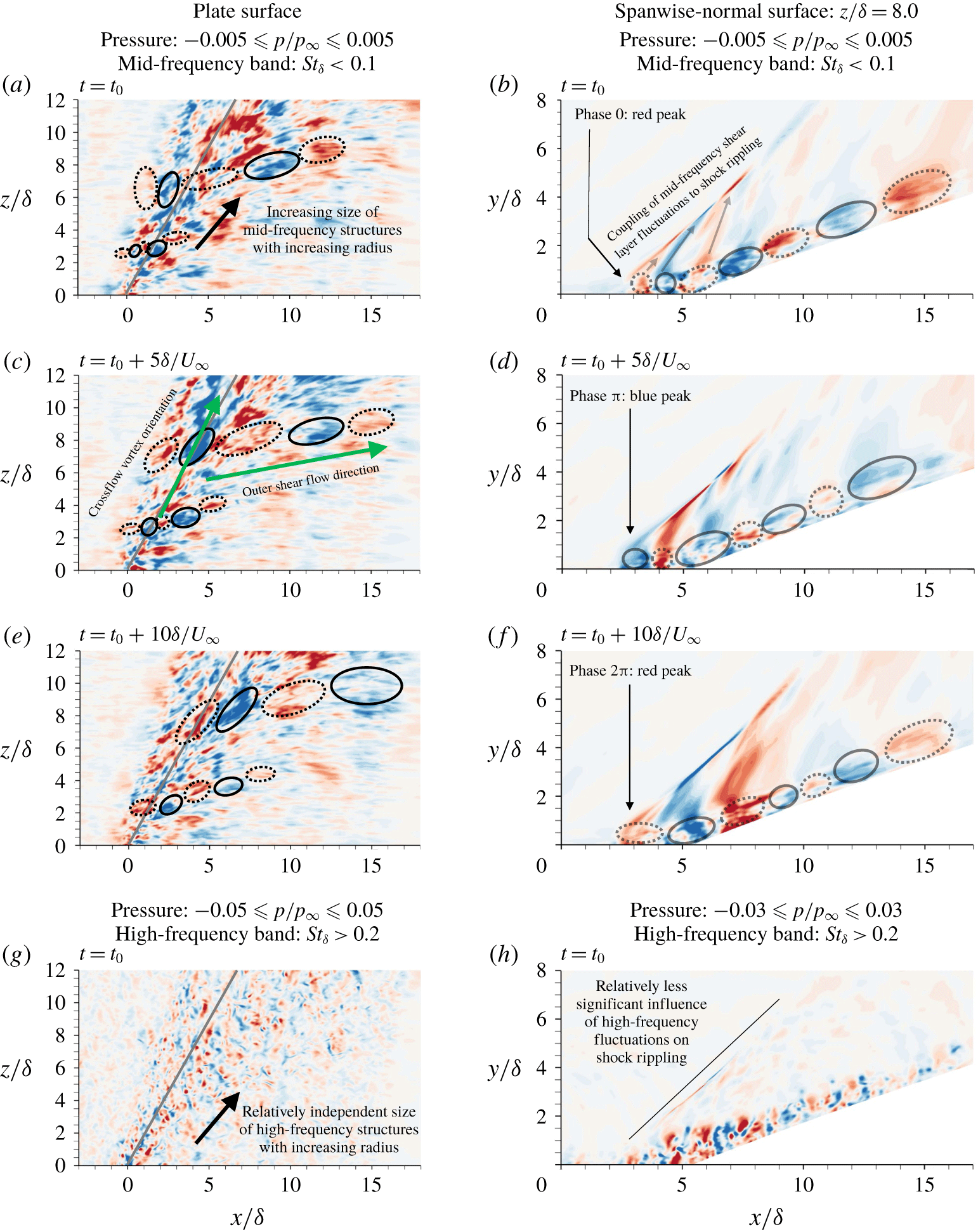
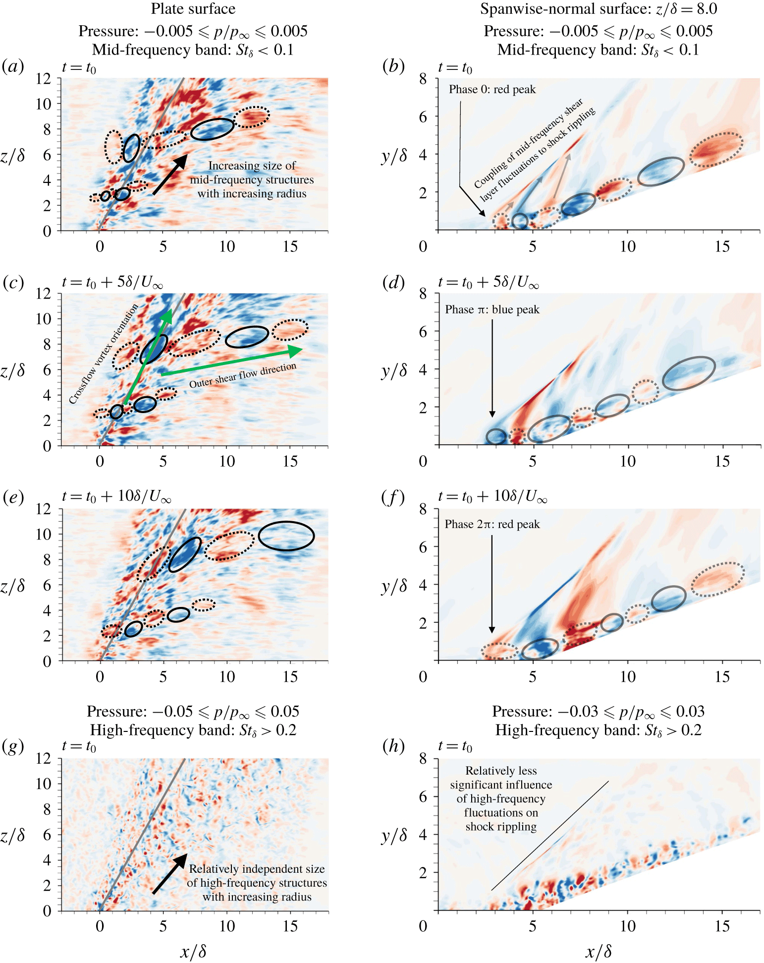
SCR: band-pass-filtered pressure fluctuations for  $22.5^{\circ }$ compression,
 $30.0^{\circ }$ sweep interaction. Spatial coordinates normalized by incoming boundary-layer thickness. Convective shear-layer coherence in the mid-frequency band is evident in (a–f). Convective but less coherent high-frequency unsteadiness is evident in (g,h). Annotations track the evolution of high (red) and low (blue) extrema pressures through consecutive panels.
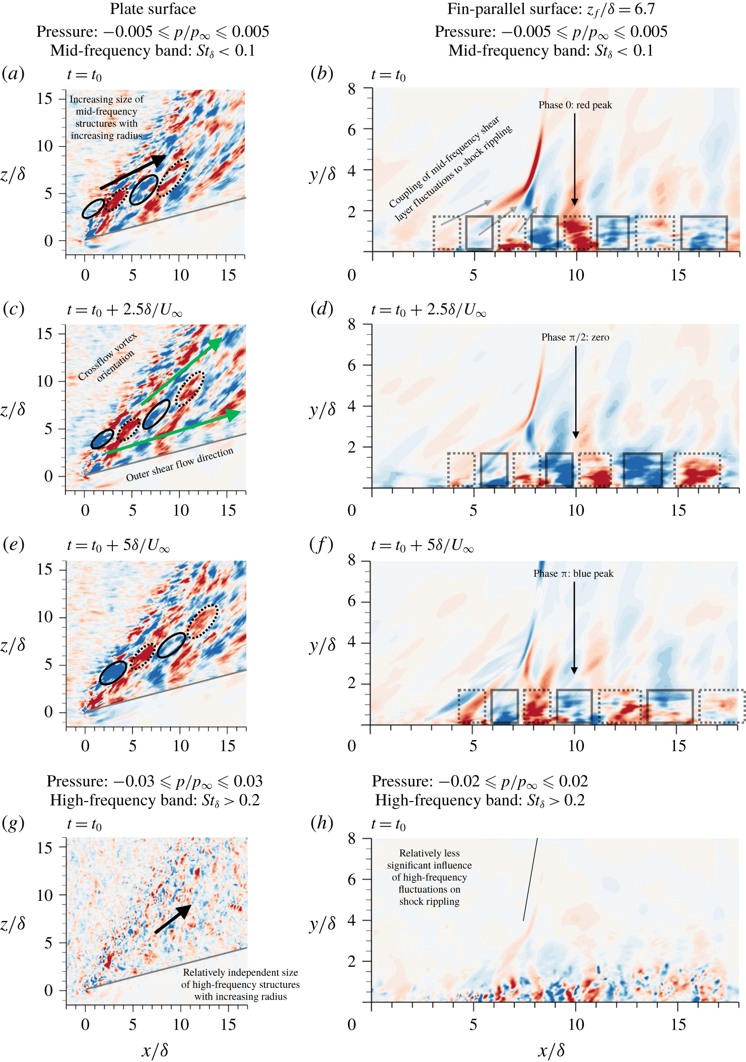
SF: band-pass-filtered pressure fluctuations for  $15.0^{\circ }$ sweep interaction. Spatial coordinates normalized by incoming boundary-layer thickness. Convective shear-layer coherence in the mid-frequency band is evident in (a–f). Convective but less coherent high-frequency unsteadiness is evident in (g,h). Annotations track the evolution of high (red) and low (blue) extrema pressures through consecutive panels.
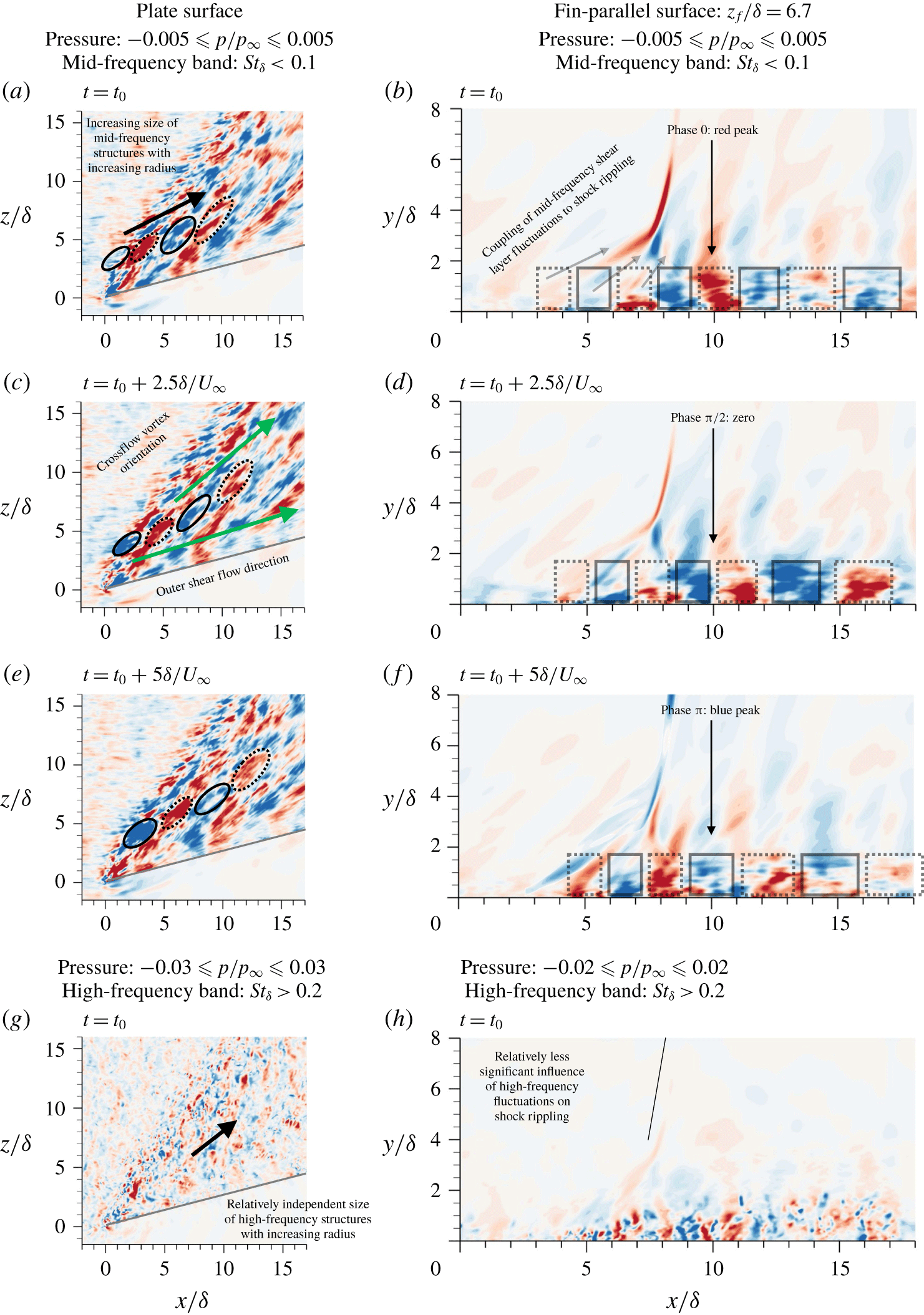
In this section, to illustrate the spatio-temporal nature of the fluctuations associated with the prominent frequency bands observed in the spectral analysis of § 4.1, a band-isolation analysis of the unsteady flow is performed for the SCR and SF interactions. For this purpose, a series of low-pass, finite-impulse-response, window-based filters are applied in sequence to obtain a complete band-isolated basis for the instantaneous flow (Adler & Gaitonde Reference Adler and Gaitonde2018a). Figures 10 and 11 describe the structure of flow features observed via pressure fluctuations in the high-frequency  $(St_{\unicode[STIX]{x1D6FF}}>0.2)$ and mid-frequency
 $(0.01<St_{\unicode[STIX]{x1D6FF}}<0.1)$ bands for the reference interactions: the (
 $22.5^{\circ }$ compression,
 $30.0^{\circ }$ sweep) SCR and the (
 $15.0^{\circ }$ attack) SF, respectively. No significant content is observed in the low-frequency
 $(St_{\unicode[STIX]{x1D6FF}}<0.01)$ band for any of the swept, 3-D interactions.
The mid-frequency bands exhibit spatio-temporally coherent fluctuations that form after separation and travel through the separated shear layer, with a surface pressure footprint that largely follows the streamlines of the outer (main) shear layer. These structures are convective in nature, as demonstrated by the temporally sequential panels (a,c,e and b,d,f) of figures 10 and 11, and they continue downstream after attachment, like in spanwise-homogeneous interactions (Agostini et al. Reference Agostini, Larcheveque, Dupont, Denieve and Dussauge2012; Aubard et al. Reference Aubard, Gloerfelt and Robinet2013; Adler & Gaitonde Reference Adler and Gaitonde2018a), as demonstrated in figures 10(b,d,f) and 11(b,d,f). However, unlike spanwise-homogeneous STBLIs, these three-dimensional interactions also result in convection of the structures associated with this frequency in the spanwise direction, through the separated flow, as demonstrated in figures 10(a,c,e) and 11(a,c,e). The competing downstream and spanwise convection directions in this band interfere both constructively and destructively, leading to intermittent in-phase and anti-phase switching of pressure fluctuations in the  $x{-}z$ plane; these characteristic directions correspond, roughly, to the mean flow directions of the outer and inner shear layers, respectively. Similar to spanwise-homogeneous interactions (Agostini et al. Reference Agostini, Larcheveque, Dupont, Denieve and Dussauge2012), these convecting coherent fluctuations influence the shock through disturbance propagation to the shock wave along the local characteristic direction, resulting in mid-frequency shock unsteadiness which is correlated with the passage of these convective structures (figures 10b,d,f and 11b,d,f). The coherent size of mid-frequency content is larger for stronger interactions and for larger radius, likely because the thicker shear-layer results in larger instability wavelengths, facilitating more coherent disruption of the shock. Additionally, the convective speed
 $({\approx}0.3U_{\infty })$ of the mid-frequency coherent structures in the main separated flow near the main shock is similar between all of the configurations and is comparable with observations of mid-frequency, coherent, vortical content in spanwise-homogeneous interactions (Aubard et al. Reference Aubard, Gloerfelt and Robinet2013). However, the convective speed of the mid-frequency content in the cross-flow (underneath the main separated flow) depends on the interaction strength. For stronger interactions, in which the cross-flow is robust and less closely aligned with the main separated flow, the mid-frequency pressure fluctuations travelling in the cross-flow direction appear less coherent and disrupted by the pressure footprint from the structures in the separated flow above.
The high-frequency band contains contributions from integral- and fine-scale turbulence and is not as coherently organized as the mid-frequency band. High-frequency pressure fluctuations are shown for a representative snapshot of both the SCR and SF interactions in figures 10(g,h) and 11(g,h). In both interactions, the amplitude of this band increases locally across the separation and attachment lines as the flow is compressed through the separation and attachment shocks. After attachment, the amplitude of these fluctuations decreases; this observation is connected to the post-interaction reduction in turbulent kinetic energy. Unlike the mid-frequency fluctuations, the coherent size of these fluctuations appears relatively independent of interaction strength and radial location; this is consistent with the observation that they are associated with integral- and fine-scale turbulence seeded from the incoming turbulent boundary-layer (2-D similarity) and not a result of developing mid-scale coherent dynamics (3-D similarity).
4.2.2 Temporal autocorrelations of mid-frequency fluctuations
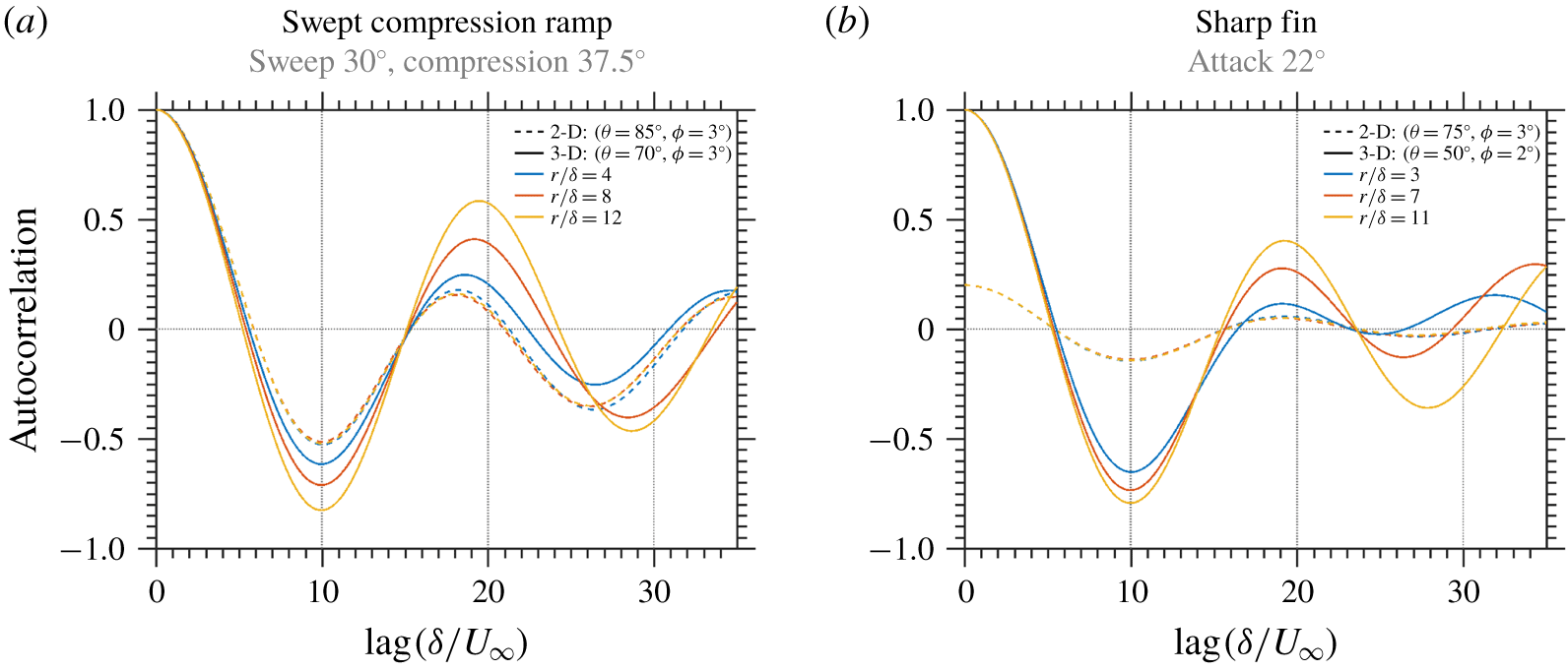
Temporal autocorrelations of low-pass-filtered pressure fluctuations  $(St_{\unicode[STIX]{x1D6FF}}\lesssim 0.05)$ in the SCR (a) and SF (b) interactions demonstrate competing 2-D and 3-D scaling laws in the mid-frequency fluctuation band. In regions of significant 3-D mean-flow symmetry (solid lines), correlations indicate a reduced rate of amplitude decay with increasing radius. However, for regions of significant 2-D mean-flow symmetry (dashed lines), the change in correlation decay rate with increasing radius is insignificant. 2-D correlations in (b) are rescaled for improved clarity.
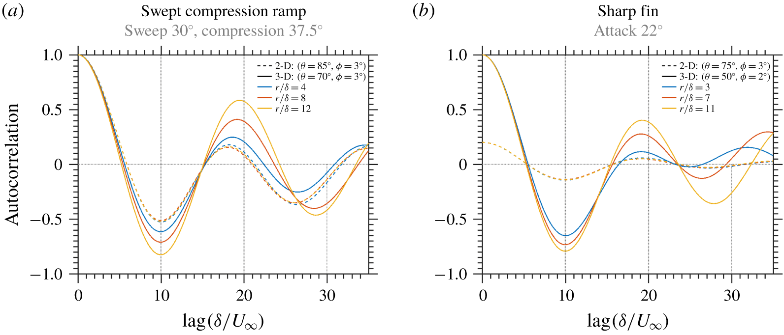
Additional quantitative evidence to distinguish 2-D from 3-D similarity scaling laws for mid-frequency fluctuations in swept, 3-D STBLIs may be gathered from the comparison of various temporal autocorrelations of pressure fluctuations. Figure 12 presents autocorrelations of low-pass-filtered  $(St_{\unicode[STIX]{x1D6FF}}\lesssim 0.05)$ pressure fluctuations for representative SCR (a) and SF (b) interactions at three different radial displacements from the VCO; the solid lines correspond to a region of the flow that exhibits 3-D mean-flow scaling in the inner (cross-flow) shear layer, whereas the dashed lines correspond to a region of the flow that exhibits 2-D mean-flow scaling in the outer (main) shear layer, just downstream of separation (Adler & Gaitonde Reference Adler and Gaitonde2019a). The low-pass filtering operation isolates pressure fluctuations associated with the lower portion of the mid-frequency band. For both interaction types, the autocorrelations associated with the flow regions of 2-D scaling are independent of the radius (spanwise homogeneous), whereas the autocorrelations associated with the flow regions of 3-D scaling are dependent on radius, with successive correlation peaks increasing in amplitude and spacing with increasing radius. Both the amplitude increase and period decrease of the 3-D autocorrelation peaks with increasing radius are consistent with the decrease in the frequency of mid-frequency unsteadiness with increasing radius (figures 6–9). Essentially, the periodic behaviour of the lower range of the mid-frequency band increases in coherence with increasing radius. Necessarily, because of the similarity of the flow velocity at each of the radial stations, these trends are also related to the spatial enlargement of mid-frequency coherence with increasing radius (figures 10 and 11).
4.3 Dynamic linear response
4.3.1 Overview of method
In addition to the phenomenological differences in unsteadiness between 2-D and 3-D STBLIs described above, there are significant differences in the underlying linear dynamics of these flows. Using the recently described method of Adler & Gaitonde (Reference Adler and Gaitonde2018a), we now compare the dynamic linear response of a representative, swept, 3-D STBLI (the SCR with  $30.0^{\circ }$ sweep and
 $37.5^{\circ }$ compression) to the results of the published 2-D impinging shock (IS) interaction (Adler & Gaitonde Reference Adler and Gaitonde2018a). The dynamic linear response results from the implicit, constrained linearization of the Navier–Stokes equations about an unsteady (LES or direct numerical simulation) base flow, subject to some perturbation of initial conditions or forcing. The implicit linearization is achieved in practice through the synchronization of two simulations, which also accounts for the linearization of sub-grid models, boundary conditions, and other implicit aspects of the numerical method. This method of stability analysis may be classified as fully three-dimensional in space and non-modal (Schmid Reference Schmid2007; Theofilis Reference Theofilis2011). The analysis is fully 3-D, in that three non-homogeneous spatial dimensions are assumed for the base flow and perturbations Additionally, the base flow is assumed to vary in time, which is facilitated by the non-modal approach, through which the base flow and perturbation solutions are calculated via coupled initial value problems.
In essence, for the discretized Navier–Stokes equations  $(\boldsymbol{F})$ acting on the conserved state vector
 $(\unicode[STIX]{x1D731})$,
 $$\begin{eqnarray}\frac{\unicode[STIX]{x2202}\unicode[STIX]{x1D6F7}_{i}}{\unicode[STIX]{x2202}t}=F_{i}[\unicode[STIX]{x1D731}],\end{eqnarray}$$
the evolution of the linear perturbation to the state vector  $(\unicode[STIX]{x1D731}^{P})$ of an unsteady base flow
 $(\unicode[STIX]{x1D731}^{B})$ may be described,
 $$\begin{eqnarray}\frac{\unicode[STIX]{x2202}\unicode[STIX]{x1D6F7}_{i}^{P}}{\unicode[STIX]{x2202}t}=\frac{\unicode[STIX]{x2202}F_{i}[\unicode[STIX]{x1D731}^{B}]}{\unicode[STIX]{x2202}\unicode[STIX]{x1D6F7}_{j}^{B}}\unicode[STIX]{x1D6F7}_{j}^{P}+S_{i}[\unicode[STIX]{x1D731}^{B},\unicode[STIX]{x1D731}^{P}],\end{eqnarray}$$
with forcing term  $(\boldsymbol{S})$. In practice, the linearization is performed implicitly via the synchronized evolution of two nonlinear simulations, and the perturbations are constrained to the linear regime. The evolution of the constrained linear perturbations (denoted
 $\unicode[STIX]{x1D731}^{P_{c}}$) may be described as
 $$\begin{eqnarray}\frac{\unicode[STIX]{x2202}\unicode[STIX]{x1D6F7}_{i}^{P_{c}}}{\unicode[STIX]{x2202}t}=F_{i}[\unicode[STIX]{x1D731}^{B}+\unicode[STIX]{x1D731}^{P_{c}}]-F_{i}[\unicode[STIX]{x1D731}^{B}]-\unicode[STIX]{x1D6FC}\unicode[STIX]{x1D6F7}_{i}^{P_{c}}+S_{i}[\unicode[STIX]{x1D731}^{B},\unicode[STIX]{x1D731}^{P_{c}}]+O(\Vert \unicode[STIX]{x1D731}^{P_{c}}\Vert ^{2}),\end{eqnarray}$$
with constraining term  $(\unicode[STIX]{x1D6FC})$ and forcing term
 $(\boldsymbol{S})$; a posteriori verification is performed to ensure that the constraining strategy satisfactorily minimizes the nonlinear error term
 $(O(\Vert \unicode[STIX]{x1D731}^{P}\Vert ^{2}))$. Concerning the perturbation response to impulse, the unconstrained linear perturbations may be related to the constrained linear perturbations,
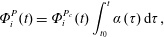 $$\begin{eqnarray}\unicode[STIX]{x1D6F7}_{i}^{P}(t)=\unicode[STIX]{x1D6F7}_{i}^{P_{c}}(t)\int _{t_{0}}^{t}\unicode[STIX]{x1D6FC}(\unicode[STIX]{x1D70F})\,\text{d}\unicode[STIX]{x1D70F},\end{eqnarray}$$
with initial condition,
 $$\begin{eqnarray}\unicode[STIX]{x1D6F7}_{i}^{P}(t_{0})=\unicode[STIX]{x1D6F7}_{i}^{P_{c}}(t_{0}).\end{eqnarray}$$
For time-dependent base flows, we generalize the classification of instabilities based on the Green’s function mapping of impulse  $(\unicode[STIX]{x1D731}^{P}(t_{0}))$ to response
 $(\unicode[STIX]{x1D731}^{P}(t))$ of the unconstrained perturbations
 $$\begin{eqnarray}\unicode[STIX]{x1D6F7}_{i}^{P}(t)={\mathcal{G}}_{ij}(t,t_{0})\unicode[STIX]{x1D6F7}_{j}^{P}(t_{0}).\end{eqnarray}$$
In this fully 3-D non-modal framework, a flow is classified as unstable if the impulse gain (the maximum norm of the Green’s function) is unbounded,
 $$\begin{eqnarray}\limsup _{t\rightarrow \infty }\Vert \boldsymbol{{\mathcal{G}}}(t,t_{0})\Vert _{\infty }\rightarrow \infty \quad \text{for some}:t_{0}.\end{eqnarray}$$
An unstable flow is additionally classified as absolutely unstable if
 $$\begin{eqnarray}\limsup _{t\rightarrow \infty }\frac{\Vert {\mathcal{G}}_{i_{0}j_{0}}(t,t_{0})\Vert _{\infty }}{\Vert \boldsymbol{{\mathcal{G}}}(t,t_{0})\Vert _{\infty }}\in (0,1]\quad \text{for some, finite, non-boundary set of}:i_{0},\,j_{0},\,t_{0},\end{eqnarray}$$
indicating that the maximum gain is sustained within a finite (spatially localized), time-independent set of degrees of freedom  $(i_{0},j_{0})$. Alternatively, an unstable flow is additionally classified as convectively unstable if
 $$\begin{eqnarray}\limsup _{t\rightarrow \infty }\frac{\Vert {\mathcal{G}}_{i_{0}j_{0}}(t,t_{0})\Vert _{\infty }}{\Vert \boldsymbol{{\mathcal{G}}}(t,t_{0})\Vert _{\infty }}=0\quad \text{for all, finite, non-boundary sets of}:i_{0},\,j_{0},\,t_{0},\end{eqnarray}$$
indicating that the maximum gain is not sustained within a finite (spatially localized), time-independent set of degrees of freedom; rather, the maximum gain is convective in character. Although the concepts of absolute and convective instability are often described in the context of a quasi-parallel flow, the aforementioned generalized definitions allow for analogous concepts to be discussed in the context of a 3-D unsteady flow. Similarities between the quasi-parallel and 3-D descriptions of absolute and convective instability exist in both the Green’s function definitions as well as in the qualitative behaviour of perturbation evolution. Similar to the classical qualitative descriptions of these phenomena in quasi-parallel flow, the dynamic linear impulse response of an absolutely unstable 3-D flow exhibits spatially bounded, self-sustaining perturbations, seemingly driven by an internal (oscillator-like) dynamics, whereas the convectively unstable 3-D flow exhibits convective perturbations, which are necessarily fed by an external source for sustenance, and are seemingly driven by the flow amplifying or filtering the externally introduced perturbations.
As discussed in detail in by Adler & Gaitonde (Reference Adler and Gaitonde2018a), the constraining term in (4.3) is chosen such that
 $$\begin{eqnarray}\Vert \unicode[STIX]{x1D731}^{P_{c}}(t)\Vert _{\infty }=\Vert \unicode[STIX]{x1D731}^{P_{c}}(t_{0})\Vert _{\infty }\;\Longrightarrow \;\Vert \boldsymbol{{\mathcal{G}}}^{c}(t,t_{0})\Vert _{\infty }\sim O(1)\quad \text{for all}:t,\,t_{0},\end{eqnarray}$$
where  $\Vert \boldsymbol{{\mathcal{G}}}^{c}(t,t_{0})\Vert _{\infty }$ represents the gain of the constrained system,
 $$\begin{eqnarray}\unicode[STIX]{x1D6F7}_{i}^{P_{c}}(t)={\mathcal{G}}_{ij}^{c}(t,t_{0})\unicode[STIX]{x1D6F7}_{j}^{P_{c}}(t_{0}).\end{eqnarray}$$
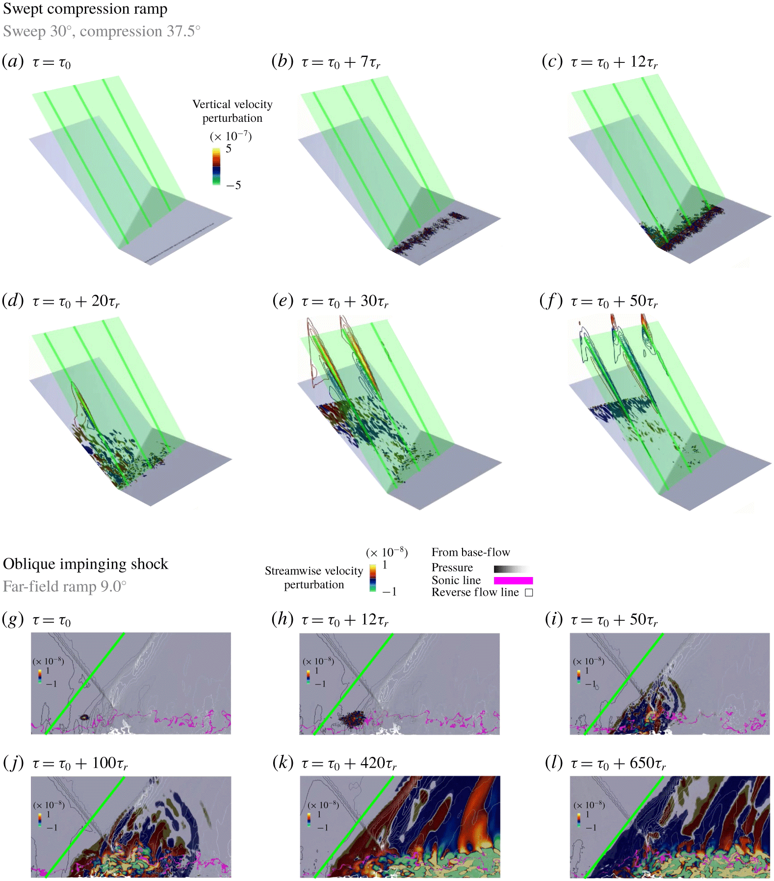
Thus, an absolute instability in the constrained system is identified by a self-sustaining (finite perturbation magnitude persisting in time) spatially localized perturbation field for some initial condition. Conversely, the absence of an absolute instability in the constrained system is identified by a locally decaying constrained perturbation field at all non-boundary locations.
4.3.2 Differences between 2-D and 3-D interactions
Demonstration of the dynamic linear response to impulse forcing for both a simple, 3-D STBLI and spanwise-homogeneous 2-D STBLI. The impulse response of the simple, 3-D interaction is not self-sustaining, instead convecting toward the domain boundaries (a–f), indicating the absence of an absolute instability, whereas the impulse response of the 2-D interaction is self-sustaining (g–l), indicating the presence of an absolute instability. Representative perturbation quantities are rendered over sequential time steps to demonstrate these contrasting responses to impulse, in which the green annotations provide a static reference to gauge shock location.
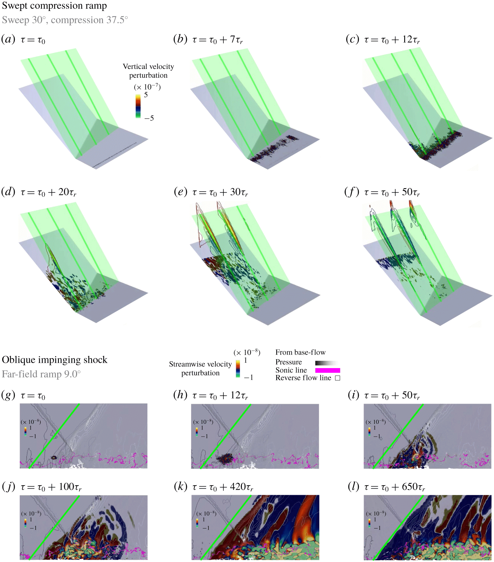
The impulse response of the 2-D impinging-shock interaction (Adler & Gaitonde Reference Adler and Gaitonde2018a) and 3-D SCR interaction are compared in figure 13. A complete, 3-D rendering is employed to visualize the SCR interaction, whereas the centreline, spanwise-normal plane is employed to visualize the IS simulation; both examples are rendered from a complete, 3-D, dynamic linear response analysis of the unsteady base flow. The impulse is introduced in both interactions through short-time, broadband, random forcing of the full, perturbation, state vector, in a spanwise-normal line upstream of the interaction. A representative perturbation quantity (vertical velocity for the SCR interaction and streamwise velocity for the IS interaction) is presented at sequential instances of time throughout the panels of figure 13, with green annotations to provide a reference shock location for both configurations along with other properties (pressure, sonic line, and reverse flow line) of the IS base flow.
The SCR interaction is perturbed in the upstream boundary layer (a), and the perturbations grow convectively in the upstream boundary layer (b), before entering the interaction region (c), where strong receptivity (large perturbation growth rate) is observed. The perturbations are processed by the interaction (d); however, no self-sustaining mechanism is observed, rather the perturbations continue to convect toward the simulation boundaries (e) and eventually start to decay in magnitude (f). This lack of self-sustaining perturbations in the simple, 3-D STBLI, is consistent with the discussion of convective instability (lack of absolute instability: equations (4.7)–(4.9)).
The IS interaction is perturbed just upstream of the separated shear layer and reflected shock (g), and the perturbations travel convectively into to interaction region (h), where strong receptivity is demonstrated (i). The perturbations are processed by the interaction (j), in which large perturbation magnitudes remain in the interaction region, relative to downstream, reflecting the strong, absolute, perturbation growth rates around the recirculation region, which ultimately result in a self-sustaining perturbation field, anchored to the interaction region, and reflective of the underlying absolute instability (4.8). The self-sustaining perturbations demonstrate a correlation with the low-frequency motion of the reflected shock wave, exhibiting high (k) and low (l) pressures for downstream and upstream shock displacement, respectively, linking the character of the absolute instability to linear restoring tendencies driving the low-frequency shock unsteadiness (Adler & Gaitonde Reference Adler and Gaitonde2018a).
The impulse responses of equilibrium turbulent boundary layers and swept, 3-D STBLIs exhibit behaviour consistent with the lack of an absolute instability, instead exhibiting only features of convective instability. Considering the mechanistic ramifications for STBLI unsteadiness, the absolutely unstable 2-D STBLI exhibits prominent low-frequency unsteadiness, whereas the convectively unstable 3-D STBLI (lacking the absolute instability) does not exhibit this prominent low-frequency unsteadiness. This raises the question as to whether the absolute instability is necessary to facilitate the low-frequency STBLI unsteadiness (two decades lower than the characteristic integral-scale boundary-layer unsteadiness and exhibiting a clear separation of scales therefrom). Our recent mechanistic description of 2-D STBLIs (Adler & Gaitonde Reference Adler and Gaitonde2018a), which describes the relationship of the linear perturbation dynamics to the evolution of the nonlinear unsteady base flow in several prominent frequency bands, suggests that the linear dynamics associated with the absolute instability is related to (and could be a primary mechanism for) the unsteady motion of the base flow in the low-frequency band. However, this does not exclude the possibility that other mechanisms also contribute to STBLI unsteadiness in that band. Concerning swept, 3-D STBLIs, the low-frequency band (comparable to the prominent low-frequency unsteadiness ubiquitously observed in 2-D STBLIs with otherwise similar flow conditions) is not observed, nor is the absolute instability, supporting the connection between the absolute instability and low-frequency STBLI unsteadiness. Further analysis will be needed to assess precisely how the convectively unstable linear dynamics contributes to the nonlinear mid-frequency unsteadiness in swept 3-D interactions.
Unfortunately, the analysis of the dynamic linear response of a convectively unstable flow (lacking an absolute instability) is not as straightforward as the analysis of an absolutely unstable flow, because the convective instability always retains a signature of the external forcing, whereas the absolute instability is ergodic (forgetting the initial forcing in the long time limit). Hence, many different responses to forcing must be accounted for in the ensemble analysis of convective instabilities, whereas ergodic ensemble averaging in time was sufficient for the absolute instability (the task of ensemble averaging for a convectively unstable flow becomes more computationally intensive). Due to the additional complexity, these analyses, apart from the simple (non-ensemble) analysis of the response to impulse, have not yet been performed. Nonetheless, this difference in the dynamic linear impulse response distinguishes the representative 2-D spanwise-homogeneous interaction from the representative 3-D swept interaction and suggests a strong connection between the exhibition of absolute instability and the manifestation of the corresponding low-frequency shock unsteadiness. This observation represents a significant advance and opens many additional avenues of research in developing a complete understanding of the interaction of the linear dynamics with the nonlinear base flow and shock unsteadiness.
5 Summary and concluding remarks
Aspects of unsteadiness in swept, 3-D STBLIs have been examined from a set of high-fidelity large-eddy simulations. The STBLI database includes a variety of SCR and SF interactions at Mach 2 free-stream conditions that have been validated with concurrent experimental efforts. The mean-flow similarity, flow unsteadiness and linear dynamics of these swept, 3-D STBLIs present significance differences from those of analogous, nominally 2-D STBLIs. Swept interactions exhibit aspects of both 2-D (spanwise homogeneous) and 3-D (quasi-conical) mean-flow similarity scaling that is coupled with a strong, cross-flow shear layer and topologically open separation structure. These features contrast with the strictly 2-D similarity scaling, absence of cross-flow, and topological separation closure of spanwise-homogeneous interactions, with ramifications leading to differences in unsteadiness between the spanwise-homogeneous (2-D) and swept (3-D) STBLIs.
The significant band of low-frequency unsteadiness (two decades below the prominent frequencies of the incoming turbulent boundary layer and demonstrating a clear separation of scales therefrom), of the type ubiquitous in spanwise-homogeneous STBLIs of comparable shock strength and separation size but exhibiting a topologically closed separation, is substantially muted in all of the SCR and SF interactions investigated. This demonstrates that (i) the properties of STBLI unsteadiness depend on the structural properties of the separation and (ii) the open topology and strong cross-flow exhibited by swept, 3-D STBLIs function to suppress a primary mechanism(s) of low-frequency unsteadiness present in unswept (spanwise-homogeneous, nominally 2-D) interactions.
A band of mid-frequency unsteadiness (one decade below the prominent frequencies of the turbulent boundary layer) is observed in all of the interactions. This is attributable to the development of coherent, convective fluctuations within the separated outer (main) shear layer and inner (cross-flow) shear layer, followed by subsequent downstream and cross-flow propagation. In both, swept, 3-D interaction types, the downstream prominence of this mid-frequency content is muted relative to spanwise-homogeneous interactions of comparable shock strength and separation size, because the 3-D flow promotes convection of these coherent structures across the span following the significant post-interaction spanwise velocity. The mid-frequency unsteadiness demonstrates a linear dependence on the separation length, exhibiting aspects of both 2-D similarity scaling (spanwise homogeneous: with  $St_{\unicode[STIX]{x1D6FF}}$ based on the incoming boundary-layer thickness) and 3-D similarity scaling (conical: with
 $St_{L}$ based on the local separation arc-length), similar to the shear-layer similarity scaling of the mean flow. The lower bound of the mid-frequency unsteadiness is described well by
 $St_{L}\sim 0.1$ (3-D scaling) and the upper bound of the mid-frequency unsteadiness is described well by
 $St_{\unicode[STIX]{x1D6FF}}\sim 0.2$ (2-D scaling). It is presently unclear if there is a practical lower bound to the 3-D mid-frequency scaling, whether the shear-layer fluctuations might continue to decrease in frequency with increasing radius, or whether this 3-D scaling might be limited by a secondary separation event or another phenomenon.
High-frequency unsteady content retains a spanwise-homogeneous (2-D) similarity scaling for frequency in all of the interactions, resulting from the initial seeding of this band by the integral-scale structures in the incoming boundary layer, which scale with the local, outer-scale Strouhal number,  $St_{\unicode[STIX]{x1D6FF}}\sim 1$. However, this high-frequency content collapses spatially with the quasi-conical (3-D) footprint of the interaction, and is largely independent of the interaction geometry parameters, except for delineation of the pre-separation, interaction, and post-attachment regions by the separation and attachment lines, through which the high-frequencies are modulated in response to decreases in local
 $U/\unicode[STIX]{x1D6FF}$. High-frequency fluctuations comprise the dominant peak unsteadiness in the premultiplied spectrum for both, swept, 3-D interaction types.
The flow structures associated with both the mid-frequency and high-frequency bands of the swept, 3-D interactions, are isolated via a band-pass filtering decomposition, to reveal the spatio-temporal nature of the coherent shear-layer and integral-scale flow features. This analysis demonstrates a correlation between the convective passage of mid-frequency, shear-layer structures and periodic rippling/corrugation of the shock structure, similar to the mid-frequency band in 2-D interactions. The more coherent nature of the mid-frequency band allows for greater relative disruption of the shock structure compared to the less orderly high-frequency band. The representative length scale of the coherent mid-frequency fluctuations is demonstrated to increase with radius, consistent with the 3-D mean flow scaling. This results in thickening of the shear layer and decrease in the lower bound of the mid-frequency unsteadiness with increasing radius. Fluctuations in this mid-frequency band exhibit convective directions aligned with both the outer (main) and inner (cross-flow) shear layers, resulting in additional mixing of 2-D and 3-D scales.
Finally, the dynamic linear response to impulse of a representative, swept, 3-D STBLI is compared to that of a spanwise-homogeneous, 2-D STBLI, to demonstrate differences in the dominant linear dynamics between the two STBLI types. The spanwise homogeneous interaction exhibits an absolute instability, resulting in self-sustaining linear perturbations with strong growth rates in the recirculation region. In contrast, the swept interaction does not exhibit an absolute instability; rather, only a convective instability that is necessarily sustained by external forcing is observed. Considering the mechanistic ramifications for STBLI unsteadiness, the absolutely unstable 2-D STBLI exhibits prominent low-frequency unsteadiness, whereas the convectively unstable 3-D STBLI (lacking the absolute instability) does not exhibit this band. This raises the question as to whether the absolute instability is necessary to facilitate the low-frequency STBLI unsteadiness. Our recent mechanistic description of 2-D STBLIs suggests that the linear dynamics associated with this absolute instability is foundational to the unsteady motion in the low-frequency band. However, it does not exclude the possibility that other mechanisms also contribute to STBLI unsteadiness in that band. Concerning swept, 3-D STBLIs, the low-frequency unsteadiness is not observed nor is the absolute instability, supporting the connection between the absolute instability and low-frequency STBLI unsteadiness.
Acknowledgements
The authors appreciate the sponsorship of the Air Force Office of Scientific Research (Monitor: Dr I. Leyva, contract FA955014-1-0167) and the Air Force Research Laboratory (AFRL) Collaborative Center for Aeronautical Sciences. M.C.A. has received support through the National Defense Science and Engineering Graduate Fellowship (NDSEG) Program as well as OSU and CTR fellowships. The simulations described were performed with grants of computer time from the Department of Defense HPCMP at the AFRL, ARL, ERDC and NAVO DSRCs. Some figures have been made with complimentary licenses of FieldView obtained from Intelligent Light through the University Partnership Program.
Declaration of interests
The authors report no conflict of interest.