

Introduction
Sentinel-2A is the first satellite of a pair projected in the Sentinel-2 mission of the European programme Copernicus and the European Space Agency (ESA). Different Sentinel missions are being deployed with satellites carrying various payloads designed for Earth Observation purposes (ESA, 2016). Images provided by Sentinel-2A are publically available for free and have 13 spectral bands with a spatial resolution ranging from 10 m to 60 m (depending on the band) and a current temporal resolution of about 10 days (depending on the latitude). Satellite Sentinel-2A was launched on June 2015 and Sentinel-2B is expected to be launched in 2017. With both satellites in orbit, the temporal resolution will be 5 days at the equator and 2–3 days at mid-latitudes. Such spatial and temporal resolutions and the availability of images free of charge make Sentinel-2 very appealing for crop monitoring in the framework of map-based precision agriculture.
Many potential applications of Sentinel-2 imagery were published before the first Sentinel-2 satellite was launched but few real applications have been described. Al-Gaadi et al. (Reference Al-Gaadi, Hassaballa, Tola, Kayad, Madugundu and Alblewi2016) used Sentinel-2 imagery to predict potato yield in different centre pivot irrigated fields getting coefficients of determination ranging from 0.47 to 0.65 when linearly correlated to NDVI. Klug et al. (Reference Klug, Schlenz, Hank, Migdall, Weiß and Danner2016) integrated Sentinel-2 data in an on-going system developed to classify crop types and to assess agricultural production. Lilienthal et al. (Reference Lilienthal, Gerighausen and Schnug2016) presented their first experiences using Sentinel-1 and Sentinel-2 imagery although they could not gather enough cloud-free Sentinel-2 images to derive reliable results. However, none of the above-mentioned papers were focused on the use of Sentinel-2 imagery at a farm level.
The present work presents the preliminary results of using Sentinel-2A data in a case study to monitor a barley field, stablish the workflow to download the images and extract vegetation indices (VIs) to create maps to correlate with the actual yield. Although it is not the scope of this communication, having vigour maps every few days would give the farmer or advisor the chance to follow the crop development, make management decisions (i.e. irrigation, fertilization and crop protection), have a feedback of the performed operations and predict yields. That will be tackled in future work.
Materials and methods
Study area
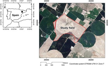
The research was carried out in a 100 ha commercial field, located in the border between the provinces of Huesca (Aragón) and Lleida (Catalonia), NE Spain (Lat 41.754223°, Long 0.370837° ETRS89, Figure 1). The field was sown with barley (Hordeum vulgare L.) on November 15th, 2015, and was harvested on June 15th, 2016. The elevation ranged from 210 to 237 m a.s.l. The slope was gentle to moderate, with an average of 5.8±4.5%. Soils of the area are classified as Typic Xerorthents (Soil Survey Staff, 2014).
Location of the case study area.

Sentinel-2 imagery
Detailed information on the Sentinel-2 mission, satellites, payloads and products can be found in Drusch et al. (Reference Drusch, Del Bello, Carlier, Colin, Fernandez and Gascon2012). The tile where the study area was located was 31TBG and the relative orbit number was 51. For this preliminary work, only the 10m-resolution bands were used i.e. Blue (B2, 490 nm), Green (B3, 560 nm), Red (B4, 665 nm) and NIR (B8, 842 nm). All available images from sowing to harvesting were collected, totalling 13 images.
Multispectral data acquisition and processing
Two approaches were followed to download and process Sentinel-2A imagery. The first was a simplified process for farmers and advisors to monitor the crop status during the season. For this purpose we used the free and open source QGIS v2.14.0 software together with the Semi-automatic Classification Plugin (SCP) v5.2.0 (Congedo, Reference Congedo2016). The advantage of using the SCP is that the user can preview and download per date and per tile single bands and correct the Sentinel-2 images in the same interface. Subsequently, the VIs can be calculated, stored and compared with other dates within the same QGIS environment. The atmospheric correction and hence the conversion of top-of-atmosphere (TOA) reflectance values into bottom-of-atmosphere (BOA) is done with the image-based Dark Object Subtraction (DOS1) method.
The second was a more complex approach. Images were downloaded from the official ESA repository, the Scientific Data Hub (https://scihub.copernicus.eu/dhus) and were pre-processed with the open source ESA Sentinel Application Platform (SNAP), which includes the Sentinel-2 Toolbox. Subsequently, the third party plugin Sen2Cor was used (http://step.esa.int/main/third-party-plugins-2/sen2cor) for atmospheric corrections. Sen2Cor is a prototype processor for Sentinel-2 Level-2A product generation and formatting; it performs the physical atmospheric, terrain and cirrus correction of TOA Level-1C Sentinel-2 products and creates, among other products, BOA reflectance corrected bands. Its output product format is equivalent to the Level 1C User Product: JPEG 2000 images with bands with three different resolutions, 60, 20 and 10 m.
When it comes to vegetation characterization it is important to accurately correct the atmospheric effects since small differences in crop reflectance are significant. Atmospheric corrections can be done according to two main method types: image-based and physical model-based methods. The former consider reflectance values within the image being corrected what makes correction accuracy dependent on the captured scene and inefficient in certain situations (Kaneko et al., Reference Kaneko, Aoki and Tsukada2016). The correction done in the first approach (DOS1) belong to this category and make derived VIs potentially less accurate than the obtained from physically-based corrections applied to Sentinel-2A with the Sen2Cor processor in the second approach (Congedo, Reference Congedo2016; Lantzanakis et al., Reference Lantzanakis, Mitraka and Chrysoulakis2016). The former may be useful to understand the variability of a single image while the latter may be recommended to extract VIs to be compared with other Vis or with subsequent seasons, different sensors and other agronomic data (Nazeer et al., Reference Nazeer, Nichol and Yung2014).
For this purpose, two Sentinel-2A images of the available collection were selected to be correlated with yield data. As barley was harvested on June 15th, 2016, images about 1 and 1.5 months earlier were chosen to correlate with yield data (May 1st and 21st, 2016 as May 11th was cloudy).
From the visible and near infrared BOA reflectance bands, two different red-based VIs (NDVI and WDRVI) and two green-based VIs (GRVI and GNDVI) were calculated: NDVI (Normalized Difference Vegetation Index, Equation 1, Rouse et al., Reference Rouse, Haas, Deering, Schell and Harlan1974), WDRVI (Wide Dynamic Range Vegetation Index, Equation 2, Gitelson, Reference Gitelson2004), GRVI (Green Ratio Vegetation Index, Equation 3, Sripada et al., Reference Sripada, Heiniger, White and Meijer2006) and GNDVI (Green NDVI, Equation 3, Gitelson et al., Reference Gitelson, Kaufman and Merzlyak1996).
 $$NDVI={{NIR{\rm }{\minus}{\rm }Red} \over {NIR{\rm }{\plus}{\rm }Red}}$$
 $$WDRVI_{\alpha } ={{(\alpha {\rm }\cdot{\rm }NIR{\rm }{\minus}{\rm }Red)} \over {(\alpha {\rm }\cdot{\rm }NIR{\plus}{\rm }Red)}}$$
 $$GRVI={{NIR} \over {Green}}$$
 $$GNDVI={{NIR{\rm }{\minus}{\rm }Green} \over {NIR{\rm }{\plus}{\rm }Green}}$$
where NIR is the reflectance of near infrared wavelength (Band 8), Red is the reflectance of red wavelength (Band 4), Green is the reflectance of green wavelength (Band 3) and α a weighting coefficient that can vary from 0.1 to 0.2. The WDRVI was created to improve correlations with the vegetation fraction for crops such as wheat, soybean and maize, thereby enabling a more robust characterization of the physiological and phenological characteristics of the crop (Gitelson, Reference Gitelson2004). In the present study, we created two WDRVI indices using α=0.1 (WDRVI0.1) and α=0.2 (WDRVI0.2) trying to find the best correlation with barley yield.
Yield data
Yield data were acquired by means of a Ceres 8000i monitor (RDS Precision Farming System) installed in a Massey-Ferguson 7370 PL combine harvester. The yield monitor operation principle is based on an optical sensor for measuring grain volume flow rate (l/s). The combine had a header width of 6.70 m, and was equipped with tilt sensors to correct the effect of slope on the sensor readings. The monitor required the working width of the harvester to be manually adjusted to the effective width. Yield was referred to a standard grain moisture content of 13%. Outliers (yield above or below ±2.5SD) were removed from the original data file according to the criteria of Taylor et al. (Reference Taylor, McBratney and Whelan2007).
Spatial interpolation of yield data was performed with VESPER (Minasny et al., Reference Minasny, McBratney and Whelan2005), using ordinary kriging in 20 m blocks and projecting interpolated data over a regular 5 m grid. A global variogram of raw processed data was initially fitted to the exponential model, and a minimum of 90 and a maximum of 100 neighbouring yield data points were used to interpolate each point on the grid.
Statistical analysis
The study of the relationship between yield and the VIs was done in a sample of 50 randomly distributed points. The ArcMap 10.4 function ‘Create Random Points’ was used for that. Then the function ‘Extract Multi Values to Points’ was applied to create a table with the yield and VI values. Each value was distance-weighted average of the 4 neighbouring grid centre values according to the bilinear interpolation function in ArcMap, representing a 20×20 m surface. The software JMP Pro 12 (SAS Institute Inc.) was used to analyse the linear relationships between both types of variables in order to know the best VI and best date to predict the final grain yield.
Results and discussion
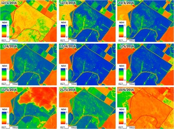
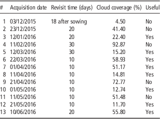
Although Sentinel-2A images were available for tile 31TBG since July 6th, 2015, the official announcement of public availability was issued on Dec 7th, 2015. The first available image after sowing (Nov 15th) was acquired on Dec 12th, 18 days after. Revisit periods were abnormally long and irregular until March 22nd, 2016 (Table 1). From then until the writing of this communication, revisit periods are 10 days on a perfectly regular basis. However, 5 out of the 13 acquired images were useless due to the presence of clouds. The field is located in the Ebro basin, characterized by long foggy events in autumn and winter. That will probably improve with the launch of Sentinel-2B. Figure 2 shows the NDVI evolution obtained according to the first and easier approach, using QGIS and the SCP plugin.
NDVI evolution along the entire season using all available and useful Sentinel-2 products. Images were processed to obtain bottom-of-atmosphere reflectance using the dark object subtraction (DOS1) correction. See digital document for colour information.

Available images, revisit time and cloud coverage for the entire crop season.

Case study: vegetation indices and yield
Although part of the yield values was lost (approx. 18.5% of the field surface), a total of 23,822 yield values were acquired by the harvester. After removing outliers, the final yield dataset was of 20,303 values, that is about 225 yield values per hectare.
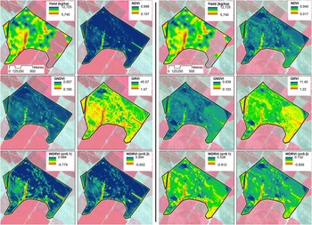
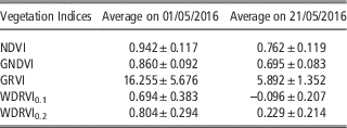
The average values of the VIs derived from the two images processed according to the second and more complex approach are shown in Table 2. The yield map and the spatial distribution of the indices for the two dates are shown in Figure 3. On the first date (May 1st, 2016) barley ears were already present and green. The index that visually shows higher variability is the GRVI and then the WDRVIs. On the second date (May 21st, 2016) the grain, and the plant had started to dry and the average values of the VIs, especially the green-based, were much lower than in the previous image (Table 2). The GRVI and WDRVIs were the indices showing higher spatial variability.
Comparison of barley grain yield and vegetation indices at two different dates: May 1st 2016 (1st and 2nd columns) and May 21st 2016 (3rd and 4th columns). Yield map is duplicated to ease the comparison. See digital document for colour information.

Average values of the vegetation indices in the two image acquisition dates.

Case study: Relationships between yield and vegetation indices
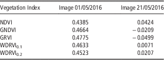
Table 3 shows the linear relationships between grain yield interpolated from the yield monitor data and the VIs calculated from the selected Sentinel-2A images. The results show that, in all cases, the correlation coefficients between yield and the VIs on May 21st were almost zero, showing no correlation. On May 1st the correlation coefficients were positive, indicating that the higher the vigour, the higher the yield. Nevertheless, the highest correlation coefficient value was only 0.48, indicating a moderate correlation.
Correlation coefficients between yield and vegetation indices for image acquisition dates 01/05/2016 and 21/05/2016 (N= 50).

The results show that correlations between yield and the VIs are moderate (May 1st, with green plants and ears) to null (May 21st). The null relationship in the second date is due to the fact that the drying process had already started unevenly in certain areas within the field. In future analysis, other images acquired on earlier dates will be processed in order to obtain better yield and VIs correlations. The best correlations were obtained with the green-based VIs (GRVI R=0.4775 and GNDVI R=0.4664), as shown in Table 3. In future analysis, other indices will be calculated using the red-edge bands of the Sentinel-2 images (Bands 5, 6, 7 and 8a) even though their spatial resolution is 20 m.
Despite the low correlation of VIs with yield data, this case study was very useful for the farmer to understand and quantify the spatial variability of vigour and yield in his field along the whole season. Once different vigour areas are identified and additional information on the soil and other agronomic parameters is retrieved, site-specific fertilization and crop protection actions could be considered for the next season.
Regarding the imagery data workflow, the first approach using QGIS v2.14.0 and the SCP v5.2.0 plugin is much more user friendly and cost-effective than the second approach. Using a single software program with plenty of online tutorials makes it easier to be used by non-experts such as farmers and/or advisors. The maps obtained are easily stored and displayed in a computer using the same GIS. This approach, although potentially more inaccurate than the second one (since it implements image-based atmospheric corrections), is enough to follow the evolution of the crop vigour along the season, looking for anomalies in the crop development or using the vigour maps as a rough feedback of agricultural operations such as irrigation, fertilization or crop protection.
The workflow of the second approach is much more complex and may prevent farmers and advisors from using it although physically-based atmospheric corrections are easier to implement in Sentinel-2 images than it is in other satellite products. Additionally, until September 28th, 2016 Sentinel-2 images had to be downloaded on a per granule basis and could easily require more than 7 GB storage capacity (since a granule is a group of several tiles in which the former Level-1C products were delivered). From October 2016 single tiles can be downloaded and they usually take around 700 MB, including a 10m-resolution RGB composite. However, the ESA SNAP software does not include image download and it has still to be done through the dedicated Copernicus website. Even though Sentinel-2 images are available in other repositories, the downloading process should be done keeping the Level-1C product characteristics and metadata in order to guarantee the compatibility with the Sen2Cor atmospheric correction plugin. Once the images are corrected and displaying BOA reflectance, SNAP can be used to calculate the vigour indices. Nevertheless, it is not a general purpose GIS and may not be convenient for farmers and/or advisors, especially if they are already using a GIS in their farms. If that is the case, the farmer and/or advisor would end using three different applications to obtain the vigour indices (a web browser to download the images, SNAP+Sen2Cor to correct them and a standard GIS to calculate the indices and store and display the maps) if they want to keep using free tools.
Conclusions
Two different workflows have been proposed to download and process the images. One is simpler but potentially more inaccurate and may be used to check infield variability and follow the crop development along the season. The second is potentially more accurate though complex and should be used to calculate vegetation indices in a more accurate and comparable way. In general, the whole process should have to be simplified for farmers and advisors to use Sentinel-2 data on a regular basis. The vegetation indices had low-medium correlation with yield. Images in earlier dates and new indices should be considered to obtain better correlations.
Sentinel-2 products are a powerful and valuable tool in precision agriculture for crop monitoring at a field, farm and even regional scale. Deeper analysis will make them also relevant in the decision making stage of the precision agriculture cycle.
Acknowledgements
This work was funded by the Spanish Ministry of Economy and Competitiveness through the project AgVANCE (AGL2013-48297-C2-2-R).