

1 Introduction
A particle released in flow undergoes a time evolution of position and velocity as governed by the net forces and torques acting on it, and its long-term behaviour is a strong function of its shape. It is widely known that for a Stokes number (Stk, the ratio of the characteristic time of the particle to that of the flow)  $\ll 1$, particles flow along streamlines with negligible inertia (Crowe, Chung & Troutt Reference Crowe, Chung and Troutt1988). However, for larger values of Stk, particle inertia becomes prominent, introducing a variety of nonlinear behaviours into the flow which can critically affect multiphase-flow applications across scales, e.g. massive oil drills with slurry transport, or lab-on-a-chip devices dealing with haemodynamics, red-blood cell fluid–structure interaction (FSI) (Fedosov, Caswell & Karniadakis Reference Fedosov, Caswell and Karniadakis2010) and micro/nano-biosensors (Prakash, Pinti & Bhushan Reference Prakash, Pinti and Bhushan2012). Other sources of nonlinearity in a system may be attributed to deformability of elastic particles/capsules (Tam & Hyman Reference Tam and Hyman1973; Kilimnik, Mao & Alexeev Reference Kilimnik, Mao and Alexeev2011), particle–particle interactions (Lee et al. Reference Lee, Amini, Stone and Di Carlo2010) and nonlinear behaviour from the fluid itself, due to non-constant viscosity for instance (non-Newtonian fluids).
In the context of fluid inertia, early studies of the passive manipulation of particles date to the mid-twentieth century when rigid neutrally buoyant spheres randomly dispersed in laminar pipe flow were observed to concentrate to annuli at  ${\approx}0.6R$ in flows with finite inertia, where
 $R$ is the pipe radius (Segre & Silberberg Reference Segre and Silberberg1961; Segré & Silberberg Reference Segré and Silberberg1962). Spheroids, bodies of revolution, ellipsoids at low-Reynolds (
 $Re$) numbers in uniform, linear shear or unbounded paraboloidal flow, respectively, were examined analytically by Oberbeck (Reference Oberbeck1876), Bretherton (Reference Bretherton1962) and Chwang (Reference Chwang1975). Subsequent studies extended these results for bounded flows with finite fluid inertia numerically for focusing of arbitrary shapes (Feng, Huang & Joseph Reference Feng, Huang and Joseph1995; de Tullio, Pascazio & Napolitano Reference de Tullio, Pascazio and Napolitano2012; Coclite et al. Reference Coclite, de Tullio, Pascazio and Decuzzi2016). Experiments by Hur et al. (Reference Hur, Choi, Kwon and Carlo2011) using disks, cylinders and
 $\boldsymbol{h}$-shaped particles further generalized the focusing characteristics of arbitrary particles. More recent studies have advanced insight into the low-
 $Re$ dynamics of irregular particles. Thaokar, Schiessel & Kulic (Reference Thaokar, Schiessel and Kulic2007) reported on the dynamics of torus-shaped particles modelled to represent polymers. They obtained a closed-form solution to the translation velocity of a rotating, force-free torus particle as a function of its slenderness ratio and angular velocity, and numerically studied its translation along a cylindrical rail. Singh et al. (Reference Singh, Koch, Subramanian and Stroock2014) studied the motion of thin axisymmetric particles placed in a low-
 $Re$ linear shear flow, where they calculate power laws for effective aspect ratios for families of shapes to control tumbling orbits, and explore shape tunability. Einarsson et al. (Reference Einarsson, Mihiretie, Laas, Ankardal, Angilella, Hanstorp and Mehlig2016) experimentally studied trajectories of micron-scale glass rods in a microfluidic channel. They examine the deviation from traditional Jeffery orbits based on the degree to which axisymmetry is broken.
These studies represent a ‘forward problem’ of the fully coupled fluid–particle system in that they detail the motion characteristics of predefined shaped particles in flow, for a given channel/flow rate. However, as the capability to manufacture complex three-dimensional shaped objects has advanced, it is also of interest to study the ‘inverse problem’, which becomes an interesting engineering question of identifying particle geometries that satisfy certain desirable motion characteristics long after release. For example, steady and non-tumbling motion of particles in inertial flow is critical for emerging particle-based applications such as imaging flow cytometry (IFC) for adherent cells. In IFC, objects of interest (typically cells in suspension) are flowed through microchannels and analysed using ultra-high-speed imaging systems, detecting structural and morphological information in high throughput. To perform this analysis on adherent cells in their naturally anchored state, cells must be anchored onto microcarriers that will be flowed through the imaging flow cytometer (Wu et al. Reference Wu, Stoecklein, Kommajosula, Lin, Owsley, Ganapathysubramanian and Di Carlo2018). Consistent microcarrier cross-sectional location and downstream velocity are necessary for effective imaging, and for sorting decisions in image-activated cell sorters which require consistent object velocity (Nitta et al. Reference Nitta, Sugimura, Isozaki, Mikami, Hiraki, Sakuma, Iino, Arai, Endo and Fujiwaki2018). Singh, Koch & Stroock (Reference Singh, Koch and Stroock2013) identified ring-shaped particles which do not tumble in shear flow, in contrast to the tumbling behaviour of axisymmetric particles reported by numerous earlier works; the particle shapes were derived as perturbations to a circular shape to obtain zero torques on the particle. Uspal & Doyle (Reference Uspal and Doyle2014) designed self-aligning and centreline-focusing characteristics of asymmetric particles in Hele-Shaw flow – specifically, ‘dumbbell’ and ‘trumbbell’ shapes.
Further motivating study of the inverse problem in fluid particle systems is the rapidly developing capabilities of particle fabrication techniques (Paulsen Reference Paulsen2017; Shaw et al. Reference Shaw, Chizari, Shusteff, Naghsh-Nilchi, Di Carlo and Hopkins2018; Yuan et al. Reference Yuan, Nagarajan, Lee, Voldman, Doyle and Fink2018; Wu et al. Reference Wu, Stoecklein, Kommajosula, Lin, Owsley, Ganapathysubramanian and Di Carlo2018). These approaches enable scalable fabrication of arbitrary-shaped microparticles, presenting an abundant landscape for the design of customized microparticles for applications in biosensing and self-assembly. Understanding and leveraging the behaviour of shaped rigid particles in flow is an increasingly relevant area of study, but the current state-of-the-art is confined to the pursuit of two different thrusts: the forward problem, which seeks to understand particle trajectories and focusing locations in the channel cross-section; and the design of particles under assumptions of zero inertia and unbounded flows for desired behaviour in flow (e.g. rotational stability and/or centreline focusing).
While much of the previously described work is useful in a limited context, there are no generalized methodologies that can be utilized for particle design in more complex scenarios, such as flows with finite fluid inertia. Here, nonlinear behaviour in the fluid–structure interaction gives rise to competing forces such as shear gradient and wall lifts, making design difficult for different flow fields and channel geometries. This motivates the work undertaken in this paper, where we formulate a framework for shape design over arbitrary flow speeds, channel and particle geometries. Subsequently, we apply this approach for design of stabilizing particles in confined flows at the channel centreline. The two main applications, which form the basis for the current work, are flow cytometry using hydrodynamic focusing with sheath flows (Golden et al. Reference Golden, Kim, Erickson, Hilliard, Howell, Anderson, Nasir and Ligler2009), and raft particles which act as stable microcarriers for biological cell specimens (Wu et al. Reference Wu, Stoecklein, Kommajosula, Lin, Owsley, Ganapathysubramanian and Di Carlo2018) for imaging flow cytometry. Sheath flow techniques use co-flowing streams to focus sample fluid to a narrow region, usually around the channel centreline for optical interrogation. However, it is well known that the centreline and its neighbourhood is an unstable region (Yang et al. Reference Yang, Wang, Joseph, Hu, Pan and Glowinski2005; Dupire, Socol & Viallat Reference Dupire, Socol and Viallat2012) for spherical- and disk-shaped particles; such particles also tumble at the off-centre stable points. We propose to improve these systems by designing stable particles that focus to the centreline for such applications, subsequent to the particles forced to neighbourhoods around the centreline using co-flows upstream of the scanning region. The inherent particle stability could reduce the sheath flow volumes required to constrict conventional particles to the channel centreline, and allow for longer maintenance of stability, after the sheath flow has been established, which is useful if longer sort decision times are needed for image based analysis. We illustrate a methodology for particle designs in two-dimensional (2-D) channel flows, for centreline focusing to perturbations about the centreline. The two parameters used to define a configuration in this study are,  $k$ (particle chord-to-channel width ratio), and,
 $Re$ (Reynolds number defined based on average fluid velocity and channel width). The proposed methods are easily generalized to three-dimensional (3-D) flow fields.
The rest of the paper is organized as follows: § 2 details the numerical methods employed for the optimization problem, § 3 details the design for centreline stability with corresponding validation using FSI, and parametric design across a range of  $k$ values and
 $Re$ values with relative comparison of the performance of the designed particles using full fluid–structure interaction simulations for centreline stability. We conclude in § 4 by framing several open questions and subsequent avenues of work. The appendices contain mathematical details of several steps in the framework: appendix A provides validation cases for the quasi-dynamic approach; appendix B details the damping coefficient calculation for an arbitrary particle; appendix C describes test cases for the optimization problem for convergence in total number of required iterations; appendix D details the convergence studies of the shape parametrization employed; and appendix E provides set-up details and validation of the FSI simulation framework.
2 Methods
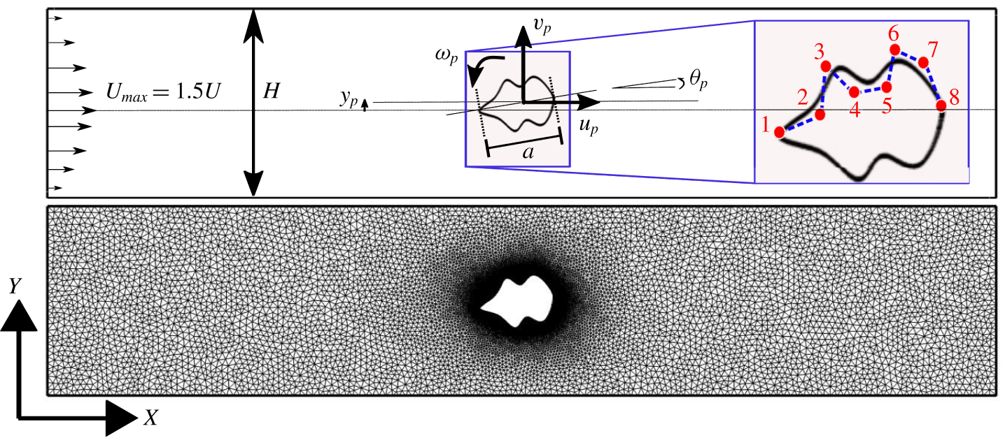
Computational model: sample geometry with 8 control points (number of variables  $(nv)=6$) and mesh for an arbitrary-shaped particle (the numbered red dots represent non-uniform rational B-spline (NURBS) control points and blue dashed lines represent the hull; confinement,
 $k=a/H,Re=\unicode[STIX]{x1D70C}UH/\unicode[STIX]{x1D707}$).

2.1 Evaluating stability of an arbitrary particle
We seek a particle design  $\boldsymbol{P}$ that is stable at the channel centreline (
 $\,y_{p}=0$), with its longitudinal axis aligned with the flow direction,
 $\unicode[STIX]{x1D703}_{p}=0$ (see figure 1 for a schematic). The two parameters that define a configuration in this study are confinement,
 $k=a/H$, and Reynolds number,
 $Re=\unicode[STIX]{x1D70C}UH/\unicode[STIX]{x1D707}$. The particle should satisfy the following two requirements:
(A) Equilibrium: the nominal configuration
 $(\,y_{p}=0,\unicode[STIX]{x1D703}_{p}=0)$ should be a force-free (and torque-free) configuration. Furthermore, we require zero lateral particle velocity ($v_{p}=0$) as well as zero angular velocity ($\unicode[STIX]{x1D714}_{p}=0$) in this configuration. This will ensure that the particle will not tumble/bob in this orientation.
(B) Stable equilibrium: the nominal configuration
$(\,y_{p}=0,\unicode[STIX]{x1D703}_{p}=0)$ should be stable to $\unicode[STIX]{x1D6FF}y$, $\unicode[STIX]{x1D6FF}\unicode[STIX]{x1D703}$ perturbations. This will ensure that the particle restores back to its nominal configuration after any perturbation.


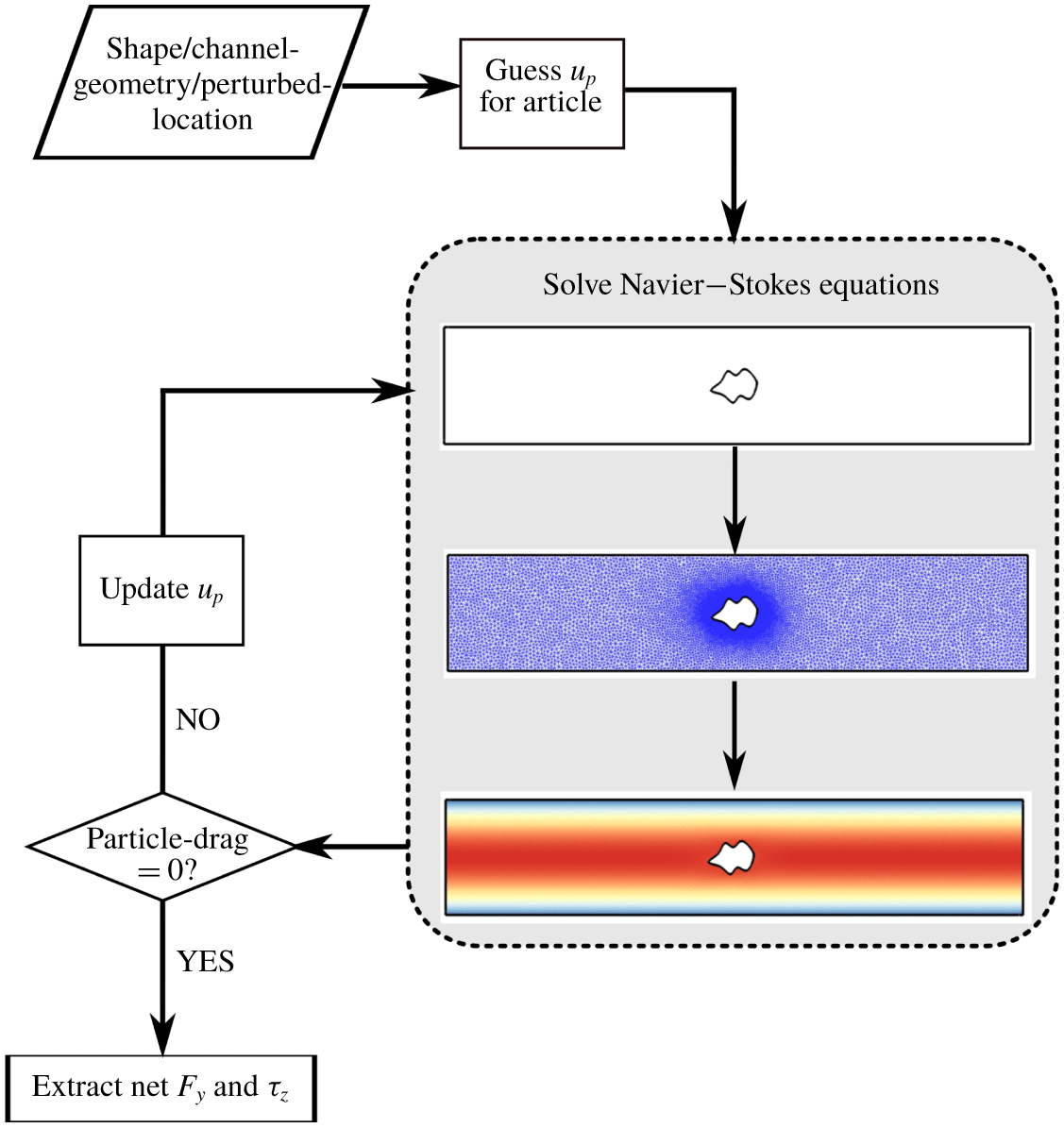
Quasi-dynamic (QD) method: for perturbed locations of the particle, identify streamwise particle velocity to yield zero drag, and compute resultant lifts and torques. See text below for further details about the QD method.

We evaluate requirement (A) using a quasi-dynamic (QD) approach (Di Carlo Reference Di Carlo2009; Kommajosula et al. Reference Kommajosula, Kim, Lee and Ganapathysubramanian2019), where the steady state Navier–Stokes equations are solved in a translating reference frame moving at  $u_{p}$, the particle streamwise velocity. The approach assumes that the particle instantaneously achieves a streamwise velocity,
 $u_{p}$, that results in the net axial force,
 $F_{x}$, becoming zero. This assumption has been previously validated for spherical particles in inertial flow (Di Carlo Reference Di Carlo2009; Kommajosula et al. Reference Kommajosula, Kim, Lee and Ganapathysubramanian2019). This force-free condition is satisfied by iteratively solving for
 $u_{p}$ (a schematic of the approach is shown in figure 2). The ‘update
 $u_{p}$’ step uses a standard Levenberg–Marquardt approach with a finite difference approximation of the Jacobian. The steady-state Navier–Stokes equations around the particle are solved to compute the fluid flow field
 $\boldsymbol{u}$, pressure field
 $p$ and the streamwise particle velocity
 $u_{p}$,
 $$\begin{eqnarray}\left.\begin{array}{@{}c@{}}\unicode[STIX]{x1D735}\boldsymbol{\cdot }\boldsymbol{u}=0\sim \mathit{incompressibility},\\ \boldsymbol{u}\boldsymbol{\cdot }\unicode[STIX]{x1D735}\boldsymbol{u}=-\unicode[STIX]{x1D735}p+\displaystyle \frac{1}{Re}\unicode[STIX]{x1D6FB}^{2}\boldsymbol{u}\sim \mathit{momentum}\,\mathit{conservation},\\ F_{x}=2\left[\displaystyle \oint _{\unicode[STIX]{x1D6E4}_{p}}\left\{-p\overline{\overline{I}}+\displaystyle \frac{1}{Re}(\unicode[STIX]{x1D735}\boldsymbol{u}+\unicode[STIX]{x1D6FB}^{\text{T}}\boldsymbol{u})\right\}\boldsymbol{\cdot }\hat{\boldsymbol{n}}\,\text{d}\unicode[STIX]{x1D6E4}\right]\boldsymbol{\cdot }\hat{\boldsymbol{i}}=0\sim \mathit{zero}\,\mathit{drag},\\[4.79993pt] u(\boldsymbol{x}\in \text{walls})=-u_{p}\sim \mathit{no}\,\mathit{slip}\,\mathit{on}\,\mathit{channel}\,\mathit{wall},\\[2.39996pt] u(\boldsymbol{x}\in \unicode[STIX]{x1D6E4}_{p})=0,v(\boldsymbol{x}\in \unicode[STIX]{x1D6E4}_{p})=0\sim \mathit{no}\,\mathit{slip}\,\mathit{on}\,\mathit{particle}\,\mathit{surface},\end{array}\right\}\end{eqnarray}$$
where  $\unicode[STIX]{x1D6E4}_{p}$ is the surface of the particle,
 $\boldsymbol{P}$. The inlet and outlet boundary conditions are chosen to have fully developed parabolic velocity profiles. The particle is far enough away from the inlet and outlet for the local disturbance around the particle to not affect the boundary velocity profiles, allowing the use of parabolic velocity profiles at the boundaries, equivalent to a particle flowing in a long channel (where the current domain is a section of that channel such that fully developed profiles can be imposed with reasonable confidence; typically the channel length is
 ${\geqslant}30$ times the characteristic length of the particle). We use an in-house finite element method framework to solve the Navier–Stokes equations with prescribed boundary conditions. Once the steady-state Navier–Stokes equations are solved, we compute the lateral force and torque acting on the particle,
 $$\begin{eqnarray}\displaystyle & \displaystyle F_{y}(\,y_{p}=0,\unicode[STIX]{x1D703}_{p}=0)=2\left[\oint _{\unicode[STIX]{x1D6E4}_{p}}\left\{-p\overline{\overline{I}}+\frac{1}{Re}(\unicode[STIX]{x1D735}\boldsymbol{u}+\unicode[STIX]{x1D6FB}^{\text{T}}\boldsymbol{u})\right\}\boldsymbol{\cdot }\hat{\boldsymbol{n}}\,\text{d}\unicode[STIX]{x1D6E4}\right]\boldsymbol{\cdot }\hat{\boldsymbol{j}}, & \displaystyle\end{eqnarray}$$
 $$\begin{eqnarray}\displaystyle & \displaystyle \unicode[STIX]{x1D70F}_{z}(\,y_{p}=0,\unicode[STIX]{x1D703}_{p}=0)=2\oint _{\unicode[STIX]{x1D6E4}_{p}}\boldsymbol{x}\times \left\{-p\overline{\overline{I}}+\frac{1}{Re}(\unicode[STIX]{x1D735}\boldsymbol{u}+\unicode[STIX]{x1D6FB}^{\text{T}}\boldsymbol{u})\right\}\!\boldsymbol{\cdot }\hat{\boldsymbol{n}}\,\text{d}\unicode[STIX]{x1D6E4}. & \displaystyle\end{eqnarray}$$
For the first requirement (equilibrium) to be satisfied, the lift  $F_{y}$ and torque
 $\unicode[STIX]{x1D70F}_{z}$ must vanish. This is a quantitative measure to ensure that the centreline position (
 $\,y_{p}=0,\unicode[STIX]{x1D703}_{p}=0$) is an equilibrium location for a given particle shape. This requirement is trivially satisfied for laterally symmetric particles located at the centreline, and we note that no flow computations are performed to check this condition at the centreline.
After assessment of requirement (A), we next quantify stability in terms of restoring forces and torques when the particle is perturbed from its stable location,  $(y_{p}=0,\unicode[STIX]{x1D703}_{p}=0)$. We again utilize the assumption of the quasi-dynamic approach, i.e. the particle instantaneously achieves a streamwise velocity,
 $u_{p}$, that results in the streamwise force
 $F_{x}$ becoming zero. A common simplification employed for creeping flows is that of the force-free particle. A scaling analysis on the equation of motion reveals that the forces vanish in the limit of
 $Re\rightarrow 0$, which implies instantaneous equilibrium of the particle in all directions for every point along its trajectory. In the case of inertial flows, however, this assumption is valid only in the streamwise direction along which the particle exhibits relatively faster responses to the underlying flow field, especially for localized perturbations around the centreline. Typical channel lengths reported in the literature for inertial migration (Di Carlo Reference Di Carlo2009) indicate smaller time scales for streamwise motion than lateral motion. This assumption has been often used, and is well validated for spherical particles (Di Carlo Reference Di Carlo2009; Kommajosula et al. Reference Kommajosula, Kim, Lee and Ganapathysubramanian2019).
We consequently use the assumptions underlying the quasi-dynamic approach as a design requirement towards enabling a tractable solution. That is, we consider a symmetric particle that is moving at steady state along the centreline. This is representative of particles reaching an equilibrium position in a long channel. We consider instantaneous perturbations about this location and calculate the restoring forces. We utilize these instantaneous restoring forces as a measure of stability. We assume that when the particle is released at its perturbed location, its non-streamwise linear ( $v_{p}$) and angular velocity (
 $\unicode[STIX]{x1D714}_{p}$) components are zero. This assumption rests on the idea that the particle is perturbed impulsively from the centreline and has yet to respond to forces arising from the now asymmetric flow field. Due to this, the particle can be assumed to have zero lateral and angular velocities when perturbed. We do not consider any time-dependent effects, computing only the restoring force
 $F_{y}$ and torque
 $\unicode[STIX]{x1D70F}_{z}$ after an impulsive perturbation. (This is a rather strong assumption, but provides a consistent estimate of the instantaneous response after an impulsive perturbation. Alternatively, the time-dependant response can be computed after an impulsive perturbation. This turns out to be extremely computationally intensive, requiring full-scale FSI simulations.) We solve the set of equations defined in (2.1) for a perturbed particle configuration
 $(\,y_{p}=\unicode[STIX]{x1D6FF}y,\unicode[STIX]{x1D703}_{p}=\unicode[STIX]{x1D6FF}\unicode[STIX]{x1D703})$, and compute the resulting lift force
 $F_{y}(y_{p}=\unicode[STIX]{x1D6FF}y,\unicode[STIX]{x1D703}_{p}=\unicode[STIX]{x1D6FF}\unicode[STIX]{x1D703})$ and torque
 $\unicode[STIX]{x1D70F}_{z}(\,y_{p}=\unicode[STIX]{x1D6FF}y,\unicode[STIX]{x1D703}_{p}=\unicode[STIX]{x1D6FF}\unicode[STIX]{x1D703})$.
A simple approach to gauging stability is to consider only the sign of the resulting lift and torque responses to perturbations. As long as the responses ensure a restoring motion towards the nominal configuration – i.e.  $F_{y}<0$ if
 $\unicode[STIX]{x1D6FF}y>0$, and
 $\unicode[STIX]{x1D70F}_{z}<0$ if
 $\unicode[STIX]{x1D6FF}\unicode[STIX]{x1D703}>0$ – the nominal configuration can be considered a stable equilibrium. The magnitude of the restorative response can be a quantitative measure of the stability, and can be used to rank order various particle shapes. However, this approach has two disadvantages: (i) it does not consider the coupled effects of a restoring force and torque on linear/angular velocities or particle displacement (i.e. it is non-intuitive whether
 $F_{y}$ should be
 ${>}0$ or
 ${<}0$ for
 $\unicode[STIX]{x1D6FF}\unicode[STIX]{x1D703}>0$, and similarly whether
 $\unicode[STIX]{x1D70F}_{z}$ should be
 ${>}0$ or
 ${<}0$ for
 $\unicode[STIX]{x1D6FF}y>0$); and (ii) it does not account for over-damped scenarios where the particle could oscillate about the nominal configuration.
We instead define simplified equations of motion for the particle based on  $F_{y}$ and
 $\unicode[STIX]{x1D70F}_{z}$, which will be used to analyse stability in response to small perturbations,
 $$\begin{eqnarray}\left.\begin{array}{@{}c@{}}\displaystyle m\frac{\text{d}^{2}y_{p}}{\text{d}t^{2}}=F_{y}(\,y_{p},\unicode[STIX]{x1D703}_{p})-\unicode[STIX]{x1D6FC}\frac{\text{d}y_{p}}{\text{d}t},\quad (\unicode[STIX]{x1D6FC}>0),\\ \displaystyle I\frac{\text{d}^{2}\unicode[STIX]{x1D703}_{p}}{\text{d}t^{2}}=\unicode[STIX]{x1D70F}_{z}(\,y_{p},\unicode[STIX]{x1D703}_{p}),\end{array}\right\}\end{eqnarray}$$
where  $\unicode[STIX]{x1D6FC}$ is the damping coefficient for the particle in the
 $y$-direction,
 $m$ is the mass of the particle and
 $I$ its moment of inertia about the
 $z$-axis. The damping coefficient for a general shape is approximated using restoring lifts on a circular particle in plane Poiseuille flow at the same
 $(k,Re)$ (see table 5). The damping coefficient is arrived at by first computing an approximate damping coefficient for a hydrodynamically equivalent circular particle assuming an under-damped motion, and then adjusting this value using a dynamic-shape factor (Leith Reference Leith1987). This calculation is detailed in appendix B. (Although it is not known a priori whether a hydrodynamically focussed circular particle exhibits rapid decay (critical damping), we assume the worst-case scenario of under-damped motion to allow for oscillations, which is the slowest to restore to equilibrium compared to critical/over-damped decay, and thus design for the same. Another important note in this regard is that we assume the damping coefficient is independent of the particle location in the channel, drawing from the Stokes drag analogy due to low transverse speed. This is again evident from the typical microfluidic channel lengths it takes for spherical beads to focus (Di Carlo Reference Di Carlo2009).) The damping coefficient ensures that there is a term in the dynamics that accounts for the velocity of the particle, thus explicitly accounting for the effect of inertia (2.4). Possible overshoots from equilibrium due to inertia are included in the Stokes drag term (which acts as a linear damper). We choose the simplest possible such term, which is a physically valid strategy used by previous researchers in inertial migration (Di Carlo Reference Di Carlo2009). Interestingly, this choice of damping coefficient is also the slowest to restore the system to equilibrium and automatically allows for oscillations about it. Thus, the present work conservatively over-designs for particle stabilization by assuming the worst-case inertial contributions to restoring and destabilizing moments. We emphasize that the presence of the damping coefficient does not alter the quality of the stability of the system (i.e. it will not make a stable particle become unstable), but it does provide a quantitative approach to rank-ordering shapes identified as stable. This choice is validated by performing long-time FSI simulations of the stable particles in subsequent sections.
The above system of two second-order equations (2.4) is converted into four first-order equations, in terms of  $(\,y_{p},\text{d}y_{p}/\text{d}t,\unicode[STIX]{x1D703}_{p},\text{d}\unicode[STIX]{x1D703}_{p}/\text{d}t)$,
 $$\begin{eqnarray}\displaystyle \left.\begin{array}{@{}c@{}}\displaystyle \frac{\text{d}y_{p}}{\text{d}t}=v_{p}\equiv f_{1}(\,y_{p},v_{p},\unicode[STIX]{x1D703}_{p},\unicode[STIX]{x1D714}_{p})\\[12.0pt] \displaystyle \frac{\text{d}v_{p}}{\text{d}t}=\frac{F_{y}(\,y_{p},\unicode[STIX]{x1D703}_{p})}{m}-\displaystyle \frac{\unicode[STIX]{x1D6FC}v_{p}}{m}\equiv f_{2}(\,y_{p},v_{p},\unicode[STIX]{x1D703}_{p},\unicode[STIX]{x1D714}_{p})\\[6.0pt] \displaystyle \frac{\text{d}\unicode[STIX]{x1D703}_{p}}{\text{d}t}=\unicode[STIX]{x1D714}_{p}\equiv f_{3}(\,y_{p},v_{p},\unicode[STIX]{x1D703}_{p},\unicode[STIX]{x1D714}_{p})\\[6.0pt] \displaystyle \frac{\text{d}\unicode[STIX]{x1D714}_{p}}{\text{d}t}=\displaystyle \frac{\unicode[STIX]{x1D70F}_{z}(\,y_{p},\unicode[STIX]{x1D703}_{p})}{m}\equiv f_{4}(\,y_{p},v_{p},\unicode[STIX]{x1D703}_{p},\unicode[STIX]{x1D714}_{p}).\end{array}\right\} & & \displaystyle\end{eqnarray}$$
This represents a first-order dynamical system which allows us to use established stability theory to rigorously quantify stability (Strogatz Reference Strogatz2018). Specifically, given a first-order differential equation  $\text{d}\boldsymbol{X}/\text{d}t=\boldsymbol{f}(\boldsymbol{X})$, we can evaluate the stability of the system about a (hyperbolic) equilibrium point
 $\boldsymbol{X}_{\mathbf{0}}$ by linearizing the system about
 $\boldsymbol{X}_{\mathbf{0}}$. The linearized system about the equilibrium point is given by
 $\text{d}\boldsymbol{X}/\text{d}t=\unicode[STIX]{x1D63C}\boldsymbol{X}$, where
 $\unicode[STIX]{x1D63C}$ is the Jacobian of the system expressed as
 $$\begin{eqnarray}\unicode[STIX]{x1D63C}=\left(\frac{\unicode[STIX]{x2202}\boldsymbol{f}}{\unicode[STIX]{x2202}\boldsymbol{X}}\right)_{\boldsymbol{X}_{\mathbf{0}}}.\end{eqnarray}$$
Stability is quantified in terms of the eigenvalues of  $\unicode[STIX]{x1D63C}$. If the real parts of all eigenvalues
 $\unicode[STIX]{x1D706}_{i}$ of
 $\unicode[STIX]{x1D63C}$ are negative, the equilibrium point is considered stable. Increasingly negative eigenvalues indicate faster transit to the equilibrium after perturbation (Strogatz Reference Strogatz2018). This is in line with similar analyses used to assess the stability of settling dumbbells in prescribed flow fields (Piva & Gabbanelli Reference Piva and Gabbanelli2003; Piva & Martino Reference Piva and Martino2008).
Comparing (2.6) and (2.5), with  $\boldsymbol{X}=[y_{p},v_{p},\unicode[STIX]{x1D703}_{p},\unicode[STIX]{x1D714}_{p}]^{\text{T}}$ the resulting Jacobian is
 $$\begin{eqnarray}\displaystyle \unicode[STIX]{x1D63C} & = & \displaystyle \left[\begin{array}{@{}cccc@{}}\displaystyle \frac{\unicode[STIX]{x2202}f_{1}}{\unicode[STIX]{x2202}y_{p}} & \displaystyle \frac{\unicode[STIX]{x2202}f_{1}}{\unicode[STIX]{x2202}v_{p}} & \displaystyle \frac{\unicode[STIX]{x2202}f_{1}}{\unicode[STIX]{x2202}\unicode[STIX]{x1D703}_{p}} & \displaystyle \frac{\unicode[STIX]{x2202}f_{1}}{\unicode[STIX]{x2202}\unicode[STIX]{x1D714}_{p}}\\ \displaystyle \frac{\unicode[STIX]{x2202}f_{2}}{\unicode[STIX]{x2202}y_{p}} & \displaystyle \frac{\unicode[STIX]{x2202}f_{2}}{\unicode[STIX]{x2202}v_{p}} & \displaystyle \frac{\unicode[STIX]{x2202}f_{2}}{\unicode[STIX]{x2202}\unicode[STIX]{x1D703}_{p}} & \displaystyle \frac{\unicode[STIX]{x2202}f_{2}}{\unicode[STIX]{x2202}\unicode[STIX]{x1D714}_{p}}\\ \displaystyle \frac{\unicode[STIX]{x2202}f_{3}}{\unicode[STIX]{x2202}y_{p}} & \displaystyle \frac{\unicode[STIX]{x2202}f_{3}}{\unicode[STIX]{x2202}v_{p}} & \displaystyle \frac{\unicode[STIX]{x2202}f_{3}}{\unicode[STIX]{x2202}\unicode[STIX]{x1D703}_{p}} & \displaystyle \frac{\unicode[STIX]{x2202}f_{3}}{\unicode[STIX]{x2202}\unicode[STIX]{x1D714}_{p}}\\ \displaystyle \frac{\unicode[STIX]{x2202}f_{4}}{\unicode[STIX]{x2202}y_{p}} & \displaystyle \frac{\unicode[STIX]{x2202}f_{4}}{\unicode[STIX]{x2202}v_{p}} & \displaystyle \frac{\unicode[STIX]{x2202}f_{4}}{\unicode[STIX]{x2202}\unicode[STIX]{x1D703}_{p}} & \displaystyle \frac{\unicode[STIX]{x2202}f_{4}}{\unicode[STIX]{x2202}\unicode[STIX]{x1D714}_{p}}\end{array}\right]_{\boldsymbol{X}_{\mathbf{0}}}\nonumber\\ \displaystyle & = & \displaystyle \left[\begin{array}{@{}cccc@{}}0 & 1 & 0 & 0\\ \displaystyle \frac{1}{m}\frac{\unicode[STIX]{x2202}F_{y}(\,y_{p},\unicode[STIX]{x1D703}_{p})}{\unicode[STIX]{x2202}y_{p}} & -\displaystyle \frac{\unicode[STIX]{x1D6FC}}{m} & \displaystyle \frac{1}{m}\frac{\unicode[STIX]{x2202}F_{y}(\,y_{p},\unicode[STIX]{x1D703}_{p})}{\unicode[STIX]{x2202}\unicode[STIX]{x1D703}_{p}} & 0\\ 0 & 0 & 0 & 1\\ \displaystyle \frac{1}{I}\frac{\unicode[STIX]{x2202}\unicode[STIX]{x1D70F}_{z}(\,y_{p},\unicode[STIX]{x1D703}_{p})}{\unicode[STIX]{x2202}y_{p}} & 0 & \displaystyle \frac{1}{I}\frac{\unicode[STIX]{x2202}\unicode[STIX]{x1D70F}_{z}(\,y_{p},\unicode[STIX]{x1D703}_{p})}{\unicode[STIX]{x2202}\unicode[STIX]{x1D703}_{p}} & 0\end{array}\right]_{\boldsymbol{X}_{\mathbf{0}}}.\end{eqnarray}$$
This representation (2.7) is a generalization to higher dimensions of the 1-D case of a circular particle focusing within a straight 2-D channel, where stability is interpreted in terms of the slope of the lift-versus-transverse coordinate curve at equilibrium locations (Yang et al. Reference Yang, Wang, Joseph, Hu, Pan, Glowinski, Balachandar and Prosperetti2006). For fully 3-D flow fields, the Jacobian  $\unicode[STIX]{x1D63C}$ would be of size
 $10\times 10$, in contrast to the 2-D case where
 $\unicode[STIX]{x1D63C}$ is a
 $4\times 4$ matrix. The additional six rows (and columns) appear due to the remaining three directions; one linear (
 $z$), and two rotational (about the
 $x$ and
 $y$ axes, based on figure 1). However, for 3-D geometries that are highly confined in the depth-wise direction (along the
 $Z$ direction), a quasi-2-D approximation would permit us to formulate stability of the particle using a
 $4\times 4$ system (equations (2.7)), while still maintaining fully 3-D flow fields (Wu et al. Reference Wu, Stoecklein, Kommajosula, Lin, Owsley, Ganapathysubramanian and Di Carlo2018). We construct the Jacobian using finite difference based gradients, and assess particle stability using the real parts of its eigenvalues,
 $\unicode[STIX]{x1D706}_{i}$ (
 $1\leqslant i\leqslant 4$): if
 $\text{Real}(\unicode[STIX]{x1D706}_{i})<0(i=1,2,3,4)$ – the given equilibrium point is stable, otherwise it is unstable.
Thus, we quantitatively evaluate the stability of an arbitrarily shaped particle. We next turn to a compact parametrization of particle shape.
2.2 Shape parametrization
The shape of a particle in flow is represented using NURBS curves with B-spline basis functions (Bingol & Krishnamurthy Reference Bingol and Krishnamurthy2019). This compact representation can generate a variety of smooth shapes, with local control of curvature using control point weights. Any point on the curve  $\boldsymbol{P}$ is given as a function of the parameter
 $\unicode[STIX]{x1D709}\,(0\leqslant \unicode[STIX]{x1D709}\leqslant 1)$, as in (Hughes, Cottrell & Bazilevs Reference Hughes, Cottrell and Bazilevs2005)
 $$\begin{eqnarray}\boldsymbol{P}(\unicode[STIX]{x1D709})=\frac{\displaystyle \mathop{\sum }_{i=0}^{n}w_{i}\boldsymbol{P}_{i}N_{i,m}(\unicode[STIX]{x1D709})}{\displaystyle \mathop{\sum }_{i=0}^{n}w_{i}N_{i,m}(\unicode[STIX]{x1D709})},\end{eqnarray}$$
where  $\boldsymbol{P}_{i}=(X_{i},Y_{i})$ are the control points,
 $w_{i}$ are the control point weights and
 $N_{i,m}(\unicode[STIX]{x1D709})$ are piecewise polynomial B-spline basis functions of order
 $m\,(=4)$, given by
 $$\begin{eqnarray}\left.\begin{array}{@{}c@{}}N_{i,m}(\unicode[STIX]{x1D709})=\displaystyle \frac{\unicode[STIX]{x1D709}-t_{i}}{t_{i+m-1}-t_{i}}N_{i,m-1}(\unicode[STIX]{x1D709})+\displaystyle \frac{t_{i+m}-\unicode[STIX]{x1D709}}{t_{i+m}-t_{i+1}}N_{i+1,m-1}(\unicode[STIX]{x1D709}),\\ N_{i,1}(\unicode[STIX]{x1D709})=\left\{\begin{array}{@{}ll@{}}1,\quad & \unicode[STIX]{x1D709}\in [t_{i},t_{i+1}),\\ 0,\quad & \unicode[STIX]{x1D709}\notin [t_{i},t_{i+1}),\end{array}\right.\end{array}\right\}\end{eqnarray}$$
 $$\begin{eqnarray}\boldsymbol{T}=\{t_{0}=t_{1}=\cdots =t_{m-1}<t_{m}\leqslant t_{m+1}\leqslant \cdots \leqslant t_{n}<t_{n+1}=\cdots =t_{n+m}\},\end{eqnarray}$$
where  $\boldsymbol{T}$ defines the knot vector and knot spans that govern the continuity of the curve and its derivatives. We use a uniform knot vector with equal weights (
 $w_{i}=1$) and constrain a fixed number of control points at predefined
 $X$-locations so that they are free to move only along the
 $Y$-direction for the design problem. The NURBS curve defines the top half of the particle (when viewed along the negative
 $z$-axis), which is mirrored about the
 $XZ$ plane to complete the shape (figure 1). For any given shape, the
 $X_{i}$ values denote the interior, equally spaced
 $X$-coordinates of the variable control points for the shapes, which have the same values for all shapes,
 $Y_{i}$ values denote the interior
 $Y$-coordinates and ‘
 $nv$’ denotes the number of such control points. The two endpoints of the NURBS curve are fixed on the
 $X$-axis, so that
 $X_{nv+1}-X_{0}=1$ (non-dimensional),
 $Y_{0}=H/2$ and
 $Y_{nv+1}=H/2$. So, the shape is parametrized as
 $\boldsymbol{P}(\unicode[STIX]{x1D709};\{Y_{0},Y_{1}\ldots Y_{nv+2}\})$, for a given set of
 $Y_{i}$ values such that
 $0.1+H/2\leqslant Y_{i}\leqslant 0.5+H/2(1\leqslant i\leqslant nv)$. Additionally, before any perturbations, we place the shape such that its centroid coincides with the centre of the channel in both the
 $X$ and
 $Y$ directions.
2.3 Design problem
We are interested in designing particles that exhibit stability to perturbations. We have quantified stability in terms of the eigenvalues of the Jacobian of the associated dynamical system. We frame the design problem as an optimization problem: to find parameters  $\{Y_{1},Y_{2},\ldots ,Y_{nv}\}$ that define a particle shape
 $\boldsymbol{P}$ which minimizes a cost functional. We choose the cost functional to be the maximum (real) eigenvalue of the system. The eigenvalues represent decay rates of the solution trajectories of the system. For the current system, each shape would have 4 such eigenvalues. Thus, to find stable shapes, we require that all real parts of eigenvalues be negative. We identify the least negative eigenvalue, and desire this eigenvalue to be as negative as possible. This automatically minimizes all other eigenvalues to improve overall restoration rates. Formally, the optimization is
 $$\begin{eqnarray}\underset{Y\equiv Y_{1},Y_{2},...,Y_{nv}}{\text{argmin}}\text{max}(\text{Real}(\unicode[STIX]{x1D706}_{i}(\boldsymbol{P})))+\text{Regularization}.\end{eqnarray}$$
Regularization terms are added to ensure that wiggly shapes with large curvature changes are penalized (the two types of regularization terms used are detailed in appendix D).
The computational effort in solving the Navier–Stokes equations and the subsequent eigenvalue problem leads to a costly objective function. Therefore, we use a Bayesian strategy to optimize particle shape (the Bayesian framework is described in detail in appendix C). Convergence with respect to the number of control points for shape representation is analysed first, because it is of interest to weigh significant improvements (if any) in the stability of the particle against the complexity in resolving the actual fabrication process. That is, fabrication processes like 3-D printing (Pham & Gault Reference Pham and Gault1998), stop-flow lithography (Dendukuri et al. Reference Dendukuri, Gu, Pregibon, Hatton and Doyle2007), optofluidic fabrication (Paulsen, Di Carlo & Chung Reference Paulsen, Di Carlo and Chung2015), continuous-flow lithography (Shaw et al. Reference Shaw, Chizari, Shusteff, Naghsh-Nilchi, Di Carlo and Hopkins2018) may not be able to capture fine features in the particle shape (wiggles/nooks) introduced by a larger number of control points, due to poor fabrication tolerances or physical effects such as the diffusion of a cross-linking photoinitiator, which will blur polymer precursors. We discuss the regularization and convergence aspects in appendix D. Furthermore, the number of original cost-function evaluations required for a reasonable approximation of the response surface is typically far lesser compared to that required with traditional optimization techniques, such as evolutionary algorithms. In the present context, as opposed to the usual approach of optimizing one infill criterion per update of the radial-basis surrogate, we perform asynchronous optimization using multiple infill criteria by giving a range of weights for exploration (high variance) versus exploitation (high mean), which updates the response surface at multiple points after each iteration. This enables efficient utilization of high-performance computing resources, a useful method for accelerating convergence in computationally difficult problems (the reader is directed to Pokuri et al. (Reference Pokuri, Lofquist, Risko and Ganapathysubramanian2018) for additional details).
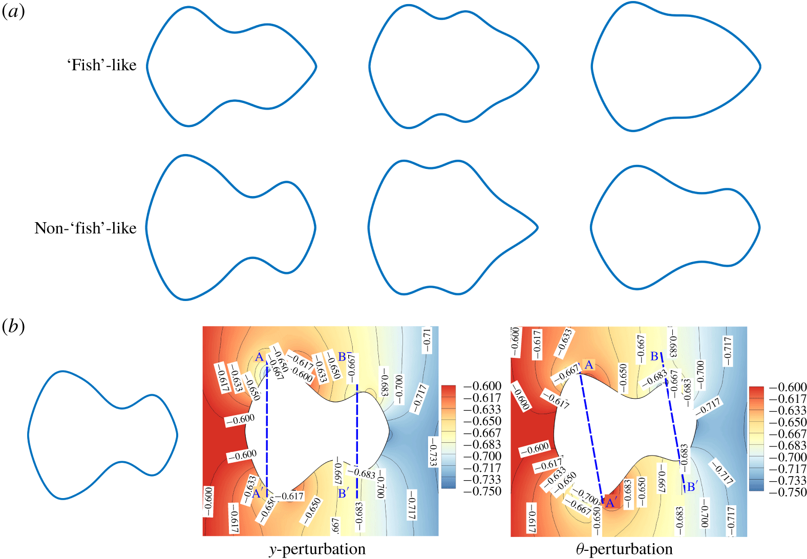
Designed particle shapes: for  $k=0.3,Re=20$: (a) ‘fish’-like and non-‘fish’ like shapes; (b) pressure contours from QD approach to perturbations in
 $y$ and
 $\unicode[STIX]{x1D703}$.

3 Results and discussion
3.1 Centreline design: $k=0.3$, $Re=20$


Particles are designed for local stability around the centreline at zero orientation. This means that, once particles have been guided close to the centreline upstream of the test section using existing techniques such as pinched-flow fractionation (Yamada, Nakashima & Seki Reference Yamada, Nakashima and Seki2004), they will locally focus and remain rotationally stable at the centreline. Families of fish-like shapes were gathered from the optimization run for the case of  $k=0.3$,
 $Re=20$ using 8 control points (
 $nv=6$) as shown in figure 3. While the best shapes (figure 3a) for this configuration singularly appear to be variants of fishes, the entire range of stable shapes is more varied in terms of the local curvature, area, aspect-ratio, etc., with the fore–aft asymmetry for some designs not being as prominent as with the set of best shapes. This allows some leeway in the fabrication process while retaining essential self-stabilizing characteristics. The pressure fields around stable particles from QD-snapshots at perturbed locations (figure 3b) indicate prominent transverse gradients across the length of the particle, especially at the extremities (sections A–A’, B–B’). Moreover, the asymmetry in these gradients in the fore compared to the aft segments acts to stabilize such particles so that a
 $y_{p}$-perturbation leads to a negative lift, and positive torque, but a
 $\unicode[STIX]{x1D703}_{p}$-perturbation gives rise to a positive lift, but negative torque. (It should be noted that an examination consisting of lift-versus-‘
 $y$’ or torque-versus-‘
 $\unicode[STIX]{x1D703}$’ trends alone would be misleading due to the inherent coupling of lift and torque as functions of ‘
 $y$’ and ‘
 $\unicode[STIX]{x1D703}$’.) It is also interesting to note the presence of features such as an intermediate ‘lobe’ at the mid-section of stable particles.
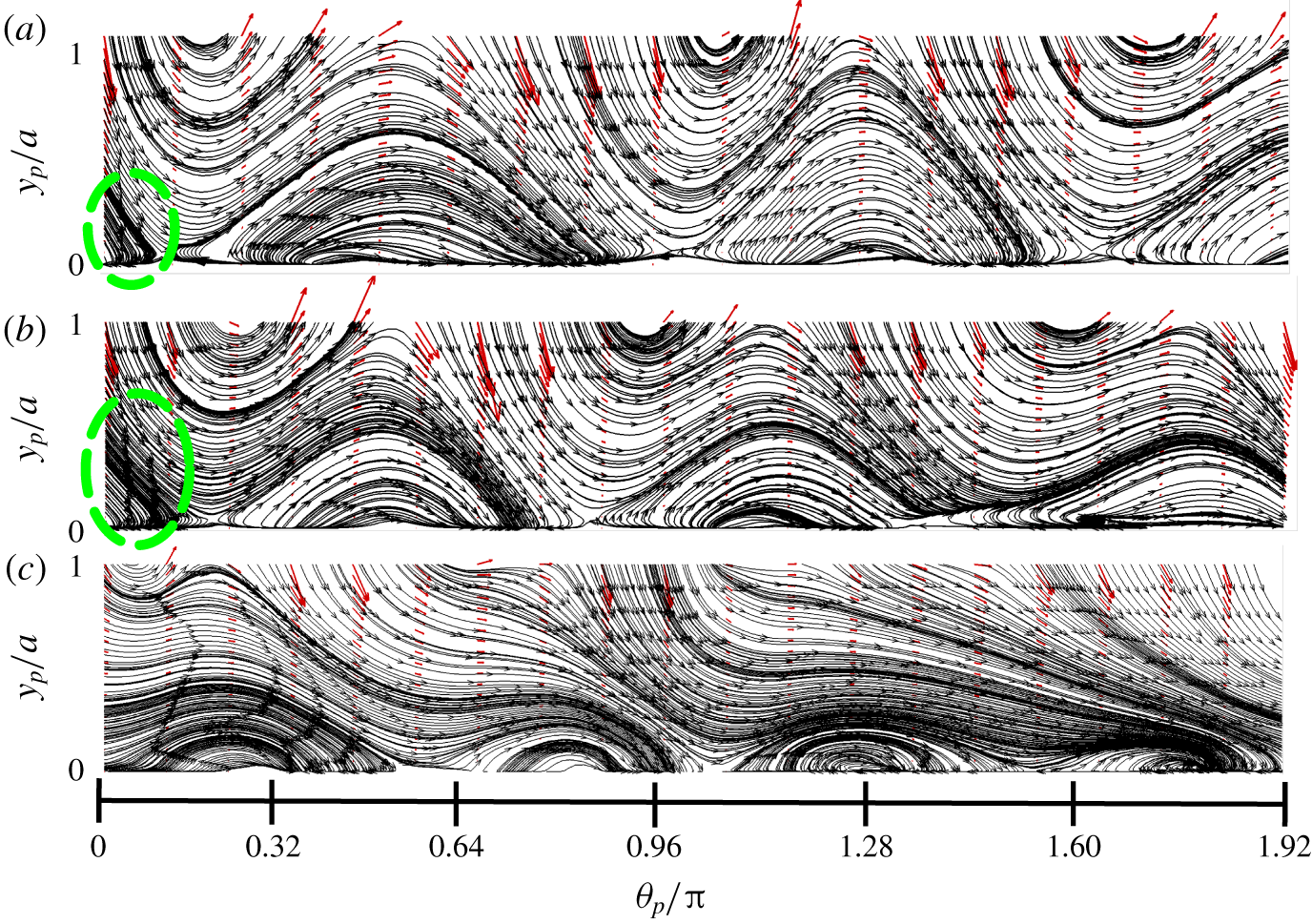
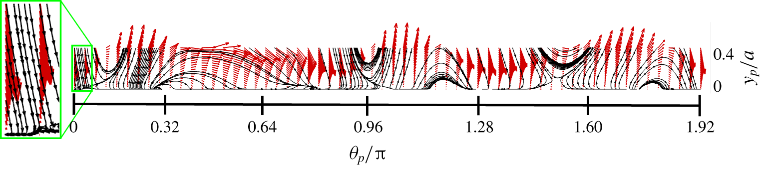
Phase portraits: in the  $y_{p}-\unicode[STIX]{x1D703}_{p}$ space for different initial release locations at
 $k=0.3,Re=20$ – (a–c): highly stable, weakly stable and unstable particles, respectively (quivers indicate vectors: (torque, lift), basins enclosed within green-dashed lines).

3.2 Global stability
The stability metric discussed previously is constructed using perturbations local to the channel centreline. However, it is also of interest to study a global notion of the particle’s tendency to focus to any stable locations in the  $y_{p}-\unicode[STIX]{x1D703}_{p}$ space, much like the cross-sectional force maps and ‘basins’ used to study particle focusing in inertial migration (Di Carlo et al. Reference Di Carlo, Edd, Humphry, Stone and Toner2009; Kim et al. Reference Kim, Lee, Wu, Nam, Di Carlo and Lee2016). For a given (
 $k$,
 $Re$) configuration, a particle is placed at different lateral and angular locations throughout the channel, and at each location, that streamwise velocity is solved which yields zero net force (see figure 2). For the current configuration (
 $k=0.3$,
 $Re=20$), we pick three shapes: highly stable, weakly stable and unstable, and construct force–torque maps and corresponding
 $\unicode[STIX]{x1D714}$-limit sets (Strogatz Reference Strogatz2018) as shown in figure 4. For any two stable particles, one is called more stable if the largest real part of its eigenvalues is more negative than that of the other. For the strongly and weakly stable shapes, we see that there are finite basins of attraction at
 $(\,y_{p},\unicode[STIX]{x1D703}_{p})=(0,0)$, which is at the channel centreline with zero inclination; for the unstable particle, however, there is no such basin. The basins of attraction for the centreline for both the stable shapes are approximately spanned by
 $0\leqslant y_{p}/a\leqslant 0.5$, and
 $-0.3\leqslant \unicode[STIX]{x1D703}_{p}/\unicode[STIX]{x03C0}\leqslant 0.15$. Practically, these basins serve as a guiding estimate of the feasible release locations of particles that lead to their focusing to the centreline. Although the current work is formulated for maximal stability of particles to perturbations after they have been focused to the centreline, the basins of attraction provide design bounds for release locations before focusing. We make a distinction here between the competing importance of having negative real eigenvalues with large magnitude but a small basin of attraction, versus eigenvalues of a modest magnitude with a large basin. While eigenvalue magnitude quantifies the speed of restoration to perturbations, the size of the basins quantifies (asymptotic) reachability from large excursions in reference to the equilibrium position. The utility of these measures would depend on specific applications, e.g. where a large basin would be needed to ensure global focusing of particles. We speculate that these two measures are generally uncorrelated, such that a weakly stable particle might have a basin size comparable to that of a strongly stable particle (see figure 4). We do not explore this distinction further in the current work.
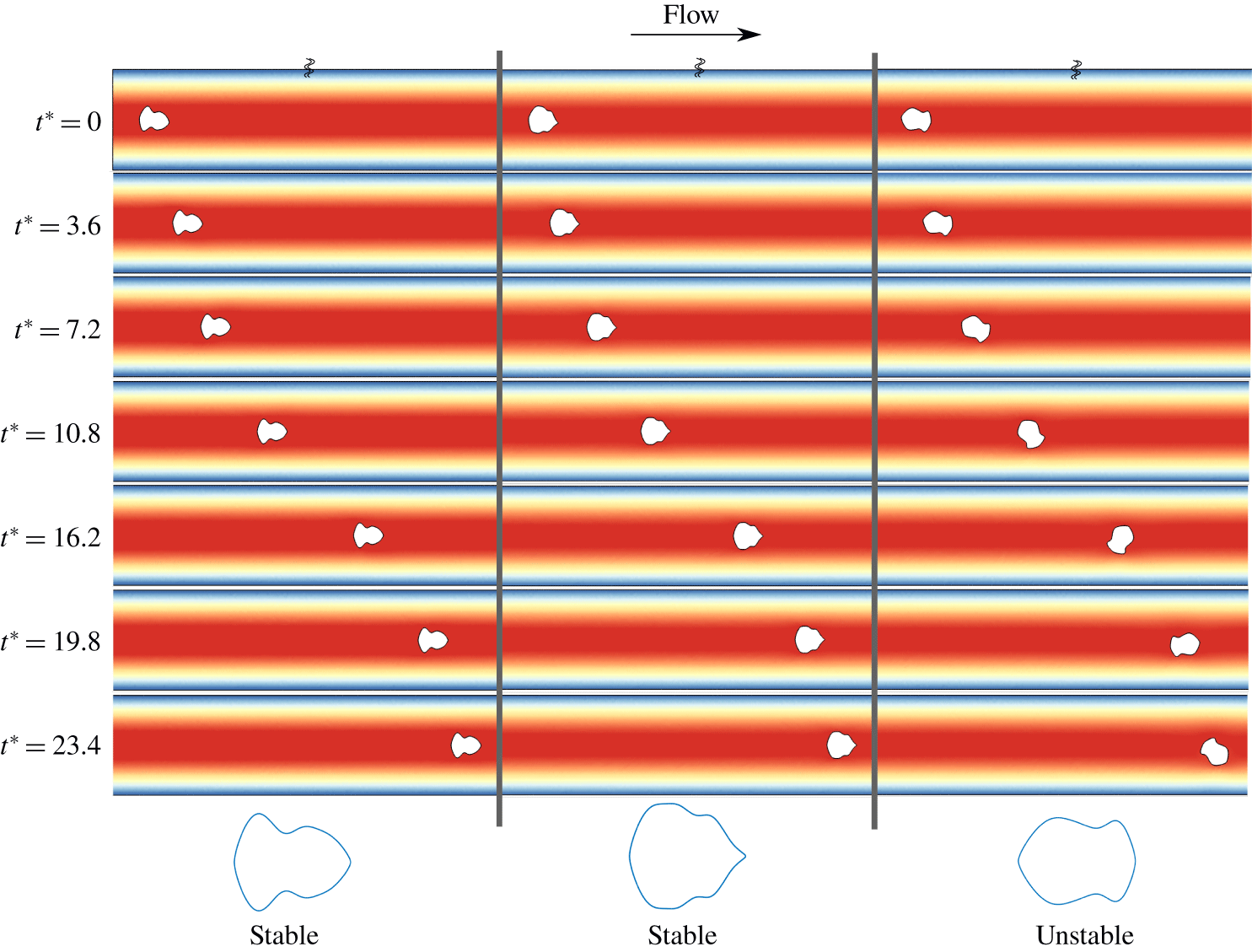
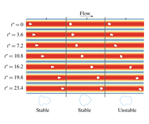
Validation with FSI: designed/randomly shaped particles are perturbed by  $-10^{\circ }$ at the centreline and flowed computationally to observe their linear/angular positions over time for
 $k=0.3,Re=20$ – on the left and the middle, highly stable and weakly stable; on the right, a randomly shaped, unstable particle (coloured by fluid-velocity contours,
 $t^{\ast }=tU/H$, denotes non-dimensional time).

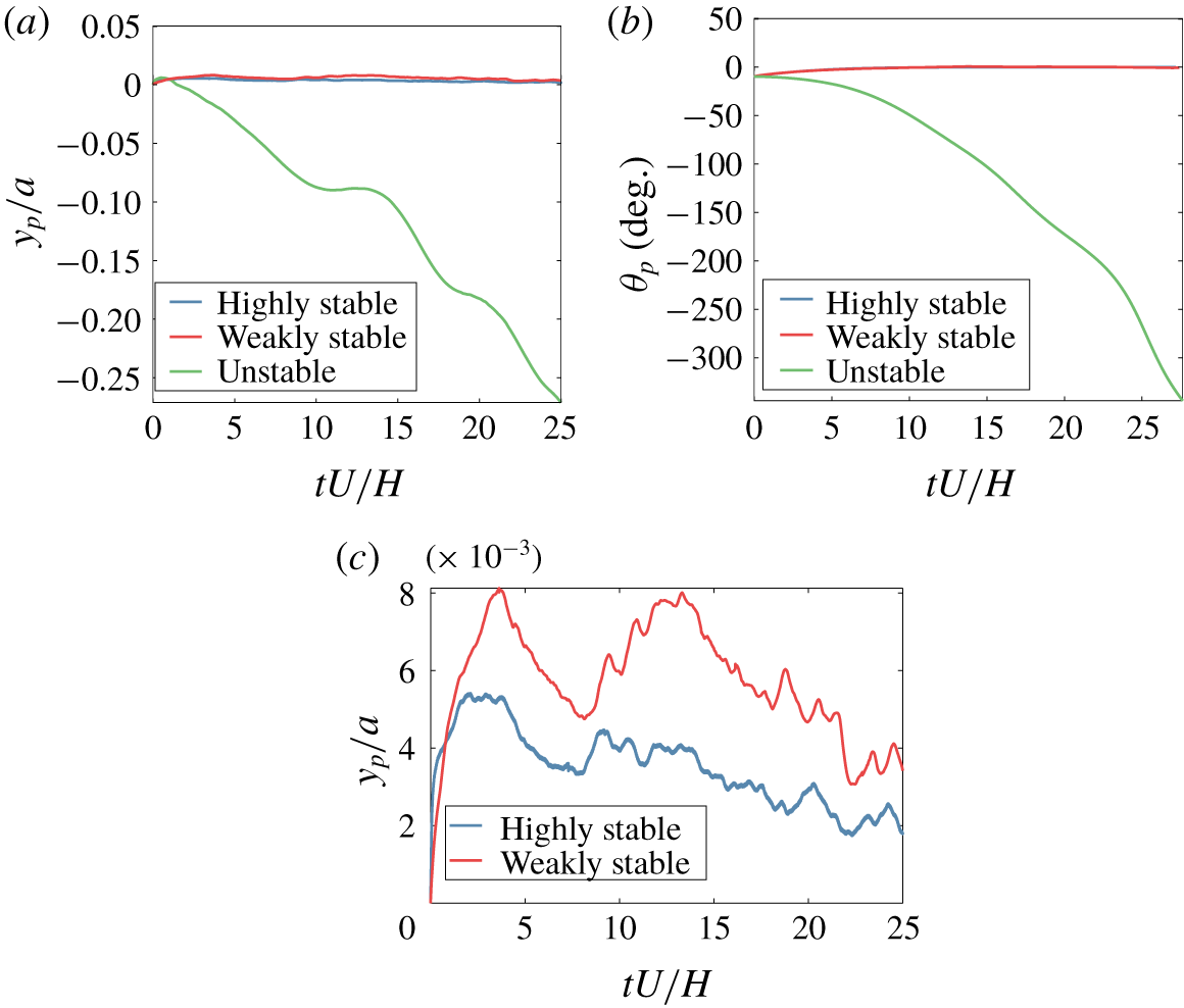
We demonstrate the behaviour of the three types of shapes in transient, fully coupled FSI simulations for a release location of  $(\,y_{p},\unicode[STIX]{x1D703}_{p})=(0,-10^{\circ })$ (simulation details in appendix E). The visuals for these simulations are shown in figure 5 and trajectories in figure 6 (animations in movies are available at https://doi.org/10.1017/jfm.2019.1007). We see that there is a conclusive demarcation between the time evolution of lateral and angular positions for the stable and unstable particles. Specifically, the unstable particle tends to rapidly destabilize and tumble over time, drifting away from the centreline monotonically. The stable particles on the other hand, display strongly restorative trajectories (that show minimal excursions), with a displacement from the centreline that is only a fraction of the height reached by the unstable particle. More importantly, it is seen that the angular displacements asymptotically reach
 $0^{\circ }$ without oscillations, confirming the validity of the damping-coefficient estimation in relation to the rank ordering of shapes in terms of their individual stabilities. Additionally, from the lateral trajectories for the stable particles, we notice that the stability metrics are reflected well in the full physics simulations. The highly stable particle has the smallest initial overshoot from to the angular perturbation, whereas the weakly stable particle overshoots to twice as much height. However, these overshoots tend to gradually decay over time as shown in figure 6(c). In figure 5, the unstable particle was inspected with the QD-method first to check that it is unstable for both
 $0^{\circ }$ and
 $180^{\circ }$ orientations, to ensure its suitability to validate the designed stable shapes against. We picked this particular unstable shape among many others to illustrate the fact that, although the stable and unstable shapes in this case both look visually similar (as ‘fish’ shapes), stability cannot be guaranteed on qualitative arguments alone. The erratic nature of the unstable particle in both head-first and tail-first orientations is well captured in the FSI trajectories, where the particle shows no tendency to stabilize in either orientation, and the rate of tumbling builds over time. Lastly, although we provide an initial angular perturbation, the difference between the stabilizing behaviour of the highly stable versus weakly stable particles is reflected in the lateral positions over time, but not the angular alignment. This is illustrative of the fact that the motion in the
 $y_{p}$ and
 $\unicode[STIX]{x1D703}_{p}$ directions is fundamentally coupled and cannot be decoupled by examining the gradients in lift or torque alone. The eigenvalues of the stability matrix essentially achieve this by giving information about the stability of the particle, and this is consequently reflected in the trajectories which can be expressed in terms of
 $\text{e}^{-\unicode[STIX]{x1D706}_{i}t}$. Additionally, due to the inertial nature of the flow, time reversibility of stabilization is broken. However, if the flow is instantaneously reversed for a stabilized particle, the particle is flipped from its nominal orientation as designed. If the basins of attraction are large enough to contain the flipped point
 $(\unicode[STIX]{x1D703}/\unicode[STIX]{x03C0},y/a)=(1,0)$, any small perturbation would return the particle back to the stable orientation.
Validation of designed particles with transient FSI: trajectories for highly stable, weakly stable and unstable shapes ( $k=0.3,Re=20$) in (a)
 $y_{p}-$trajectories; (b)
 $\unicode[STIX]{x1D703}_{p}-$trajectories; and (c)
 $y_{p}-$trajectories for highly versus weakly stable particles (released at the channel centreline,
 $y_{p}=0$, for an angular perturbation of
 $\unicode[STIX]{x1D703}_{p}=-10^{\circ }$, animations in Movie 1, Movie 2, Movie 3, respectively).

3.3 Centreline design: $k=0.1{-}0.4$, $Re=10{-}80$


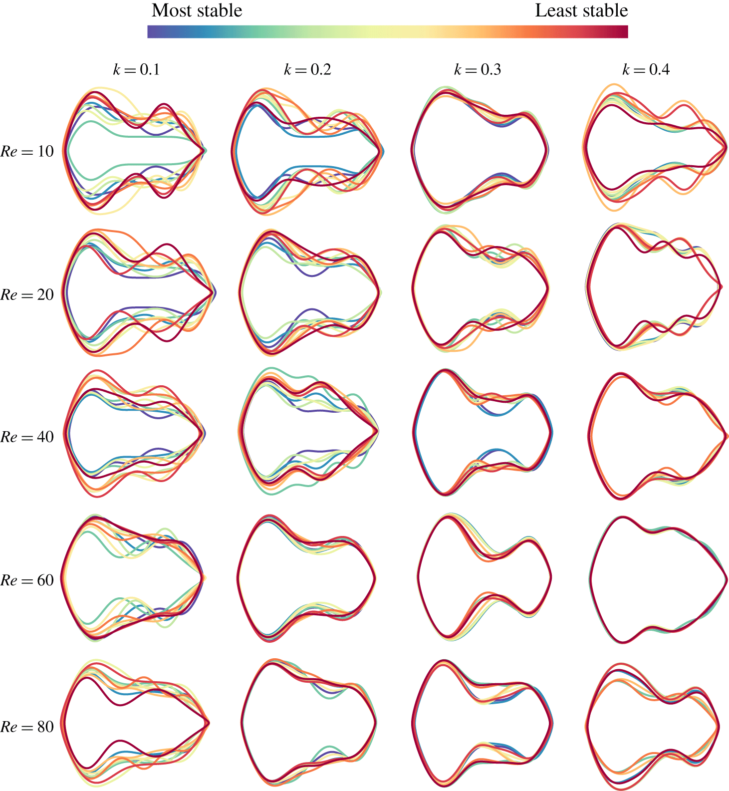
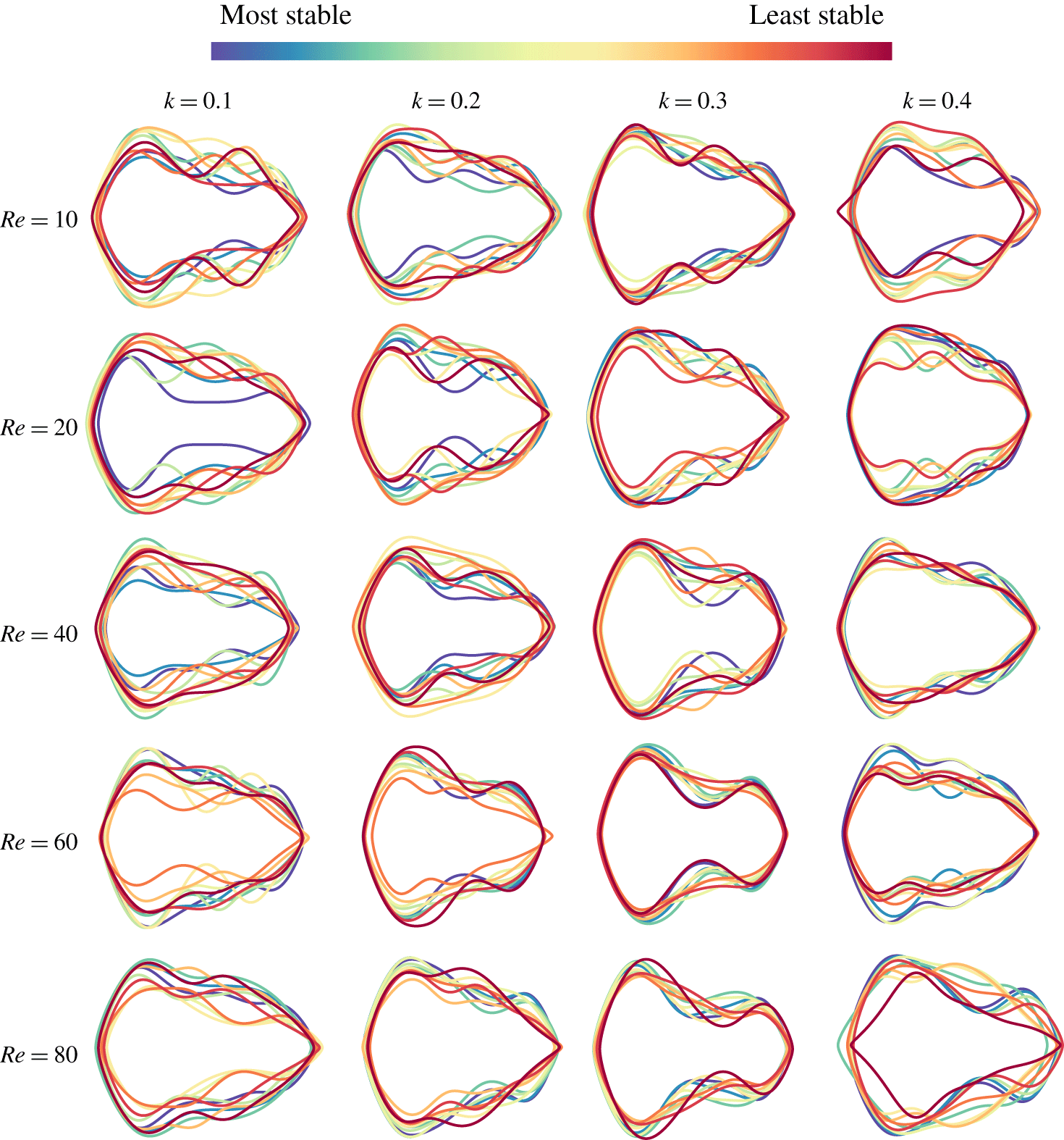
We next design families of stable shapes (figure 7, figure 8) for a parametric range of the flow parameters,  $0.1\leqslant k\leqslant 0.4$, and
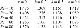
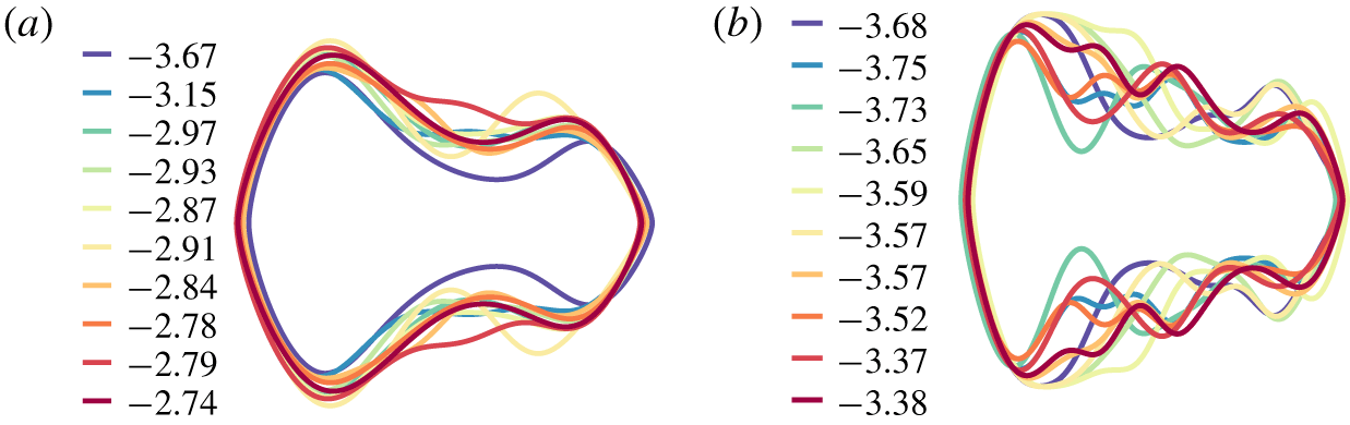
 $10\leqslant Re\leqslant 80$. These families indicate that the most-stable particles are classes of ‘fishes’/‘bottles’/‘dumbbells’. It is observed that reduced confinement and
 $Re$ tend to result in high aspect ratio rod-like shapes, whereas increased confinement and
 $Re$ tend to favour low-to-moderate aspect ratio shapes (table 1). The asymmetric make up of the rod-like particles would seem to be a consequence of smaller velocity gradients across the particle, which the lobe and longer ‘lever arm’ of the particle would leverage to realign the particle after being perturbed. The trends indicate that in general, there is a good amount of variability between all possible stable shapes for any given (
 $k$,
 $Re$) configuration (see figure 8), suggesting multiple local minima in the global landscape of the chosen cost function. However, among optimally stable shapes, a large variance is only seen in families designed for low confinements (see figure 7). Additionally, it is seen that shapes which are optimal in the orientation reported here (
 $\unicode[STIX]{x1D703}_{p}=0^{\circ }$) are highly unstable in the
 $\unicode[STIX]{x1D703}_{p}=180^{\circ }$ orientation, which suggests uniqueness of the preferred stable orientation in flow. We note that in figure 7, very little variation is visibly apparent among certain configurations such as
 $(k,Re)=(0.3,60),(0.4,60)$, but this trend is not preserved for configurations in
 $Re=80$. This can be attributed to the spread in the stability values among the top 10 shapes (and consequently, the shapes themselves) at each configuration, which is specific to the landscape of the cost functional. For the former configurations, this spread is quite small, while the separation is large for the latter. We verified this by running multiple optimizations for
 $(k,Re)=(0.4,60)$ with different initial sampling and infill criterion. Either way, we can conclude for each configuration that there exists a diverse family of shapes that exhibit centreline stability (figure 8), while the variation may or may not be large purely within the top designs (figure 7).
Mean aspect ratios of best shapes from figure 7.

Families of stable shapes for centreline alignment:  $0.1\leqslant k\leqslant 0.4,10\leqslant Re\leqslant 80$. The 10 most-stable shapes per configuration are shown (shapes to scale).

Families of stable shapes for centreline alignment:  $0.1\leqslant k\leqslant 0.4,10\leqslant Re\leqslant 80$. Ten shapes are shown for each (
 $k$,
 $Re$), ranging between the most stable to least stable per configuration (shapes to scale).

Phase portraits: in the  $y_{p}-\unicode[STIX]{x1D703}_{p}$ space for different initial release locations at
 $k=0.5,Re=10$ (quivers indicate vectors: (torque, lift), basins enclosed within green lines).

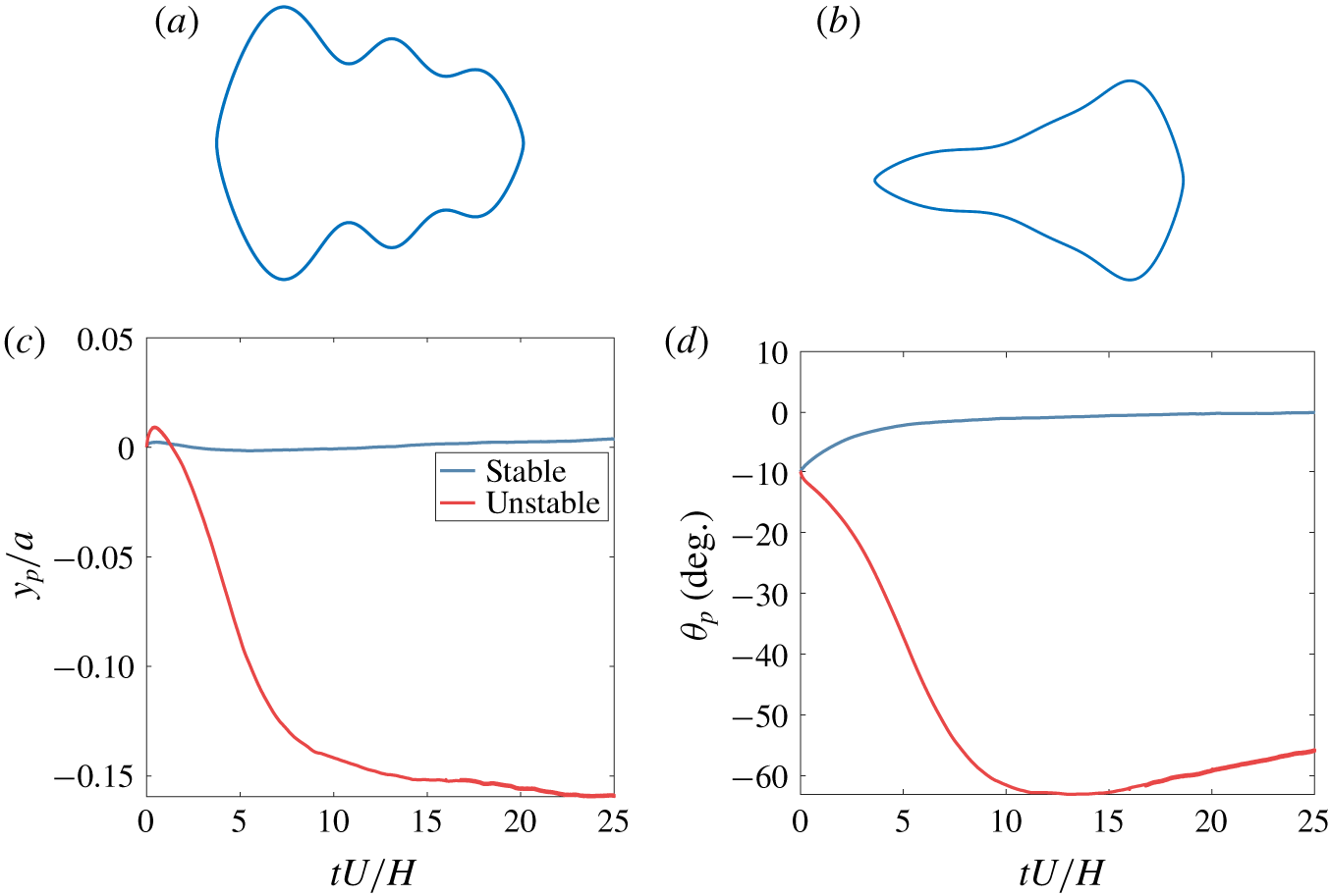
Validation with FSI: for  $k=0.4,Re=20$ (a) stable shape; (b) unstable shape; (c)
 $y_{p}$-trajectories; and (d)
 $\unicode[STIX]{x1D703}_{p}$-trajectories (released at the channel centreline,
 $y_{p}=0$, for an angular perturbation of
 $\unicode[STIX]{x1D703}_{p}=-10^{\circ }$, animations in Movie 4, Movie 5, respectively).

It is interesting to note that the stability of particles increases with an increase in either confinement or  $Re$. However, confinement seems to have a stronger effect on stability (
 $40{-}70\times ~\text{between}~k=0.1{-}0.4$) than
 $Re~(5{-}8\times ~\text{between}~Re=10{-}80)$. It is widely known that the effect of walls on particles is to retard their motion as well as exert a lateral force away from the walls (Zhang et al. Reference Zhang, Yan, Yuan, Alici, Nguyen, Warkiani and Li2016). Thus, in narrow channels it is expected that the combined effect from both sidewalls might act to significantly slow down the particle as well as constrain it to the centreline, whereas the effect of the farther wall may be comparatively insignificant in wider channels. In general, changing the confinement changes the shear rate (if particle size is kept constant), which in turn affects the torque on the particle. Classically, lift forces on spherical particles and scaling laws thereof have been derived in cases of slip velocity (and unbounded flows) and the presence of walls in linear shear flows (McLaughlin Reference McLaughlin1993; Saffman Reference Saffman1965), in Poiseuille flows for small/large particles (Asmolov Reference Asmolov1999; Di Carlo et al. Reference Di Carlo, Edd, Humphry, Stone and Toner2009; Hood, Lee & Roper Reference Hood, Lee and Roper2015) and so on. These studies exhibit a sequence of increasingly complex physics for migration arising due to the presence of shear, shear gradients, slip shear, wall effects, fluid inertia and finite particle sizes for spherical particles, and the designs shown here build upon these in the context of non-circular particles. Additionally, we see that there exist shapes which are stable across multiple (
 $k$,
 $Re$) configurations.
3.4 Stability under high confinement
We designed particles for  $k=0.5$ and
 $Re=10$ to examine basins of attraction (figure 9). From the basins for the wider channel cases (i.e. smaller
 $k$, see figure 4), we see that the basin for
 $(\,y_{p},\unicode[STIX]{x1D703}_{p})=(0,0)$ for the present configuration includes nearly the entire lateral range of release locations, and
 $-0.35\leqslant \unicode[STIX]{x1D703}_{p}/\unicode[STIX]{x03C0}\leqslant 0.1$ for release angles. This is a significant coverage compared to the wider channels, where the lateral range was restricted to a notably smaller span. This suggests applicability of the design optimization approach in this work toward global focusing, with a significant range of particle release angles and locations in narrower channels. Such basins of attraction would be even more significant for confinement ratios (
 ${\approx}0.72$) akin to those used in recent works (Wu et al. Reference Wu, Stoecklein, Kommajosula, Lin, Owsley, Ganapathysubramanian and Di Carlo2018). Furthermore, we also evaluated the stabilities of designs and basins for perturbations in
 $Re$, and
 $k$ (up to
 $\pm 3\,\%$ change), and in each case we confirmed that they are not sensitive to small changes about the design configurations. From the parametric sweep for centreline-stable particles (figure 7), we also test the performance of flowing particles for additional configurations (using FSI), varying in
 $k$, or
 $Re$ or both. Specifically, we test for response to angular perturbations –
 $(k,Re)=(0.4,20),(0.4,80)$ – as well as transverse perturbations –
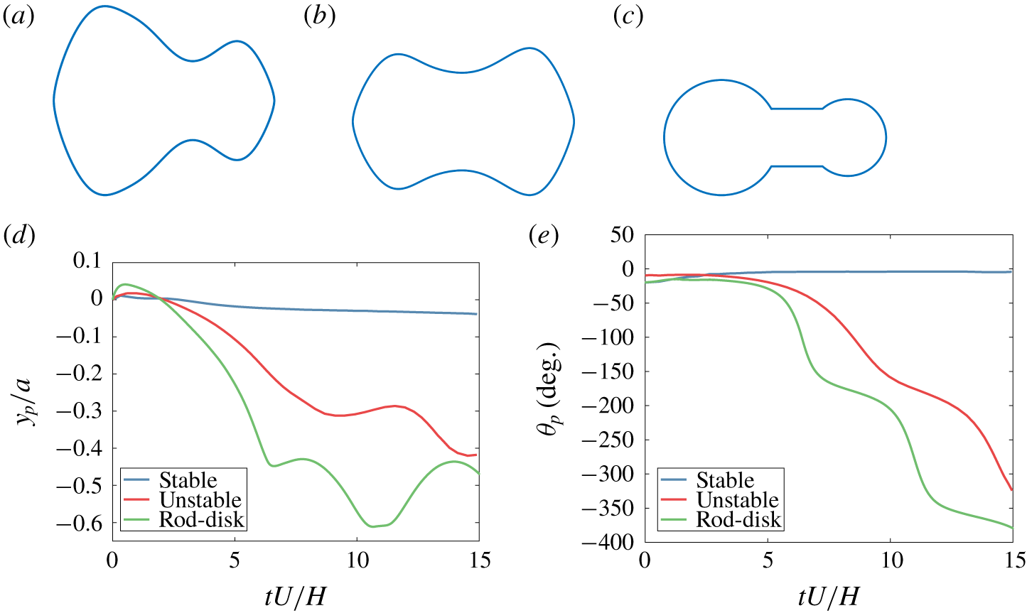
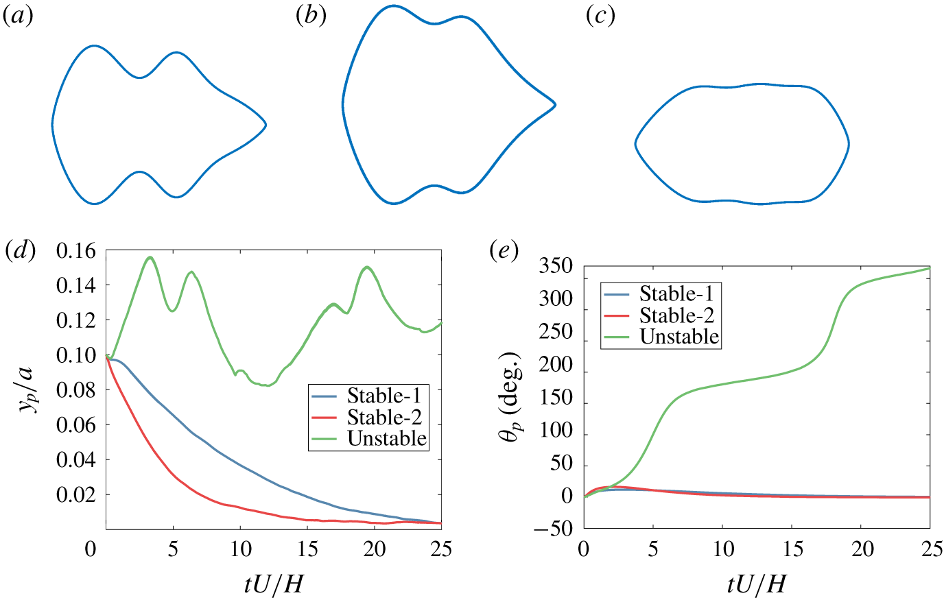
 $(k,Re)=(0.7,20)$, and trajectories are shown in figure 10, figure 11, figure 12, respectively, along with candidate shapes. It is apparent that particles restore monotonically in the direction of the initial perturbation, while the displacement in the other direction is non-monotonic, tending to shift the particle away from equilibrium at first, until stabilizing stresses begin to re-position it to the mean location. As with earlier cases, particles deemed to be unstable by our cost function drift away significantly from the centreline, accompanied by a tumbling motion. In this context, we note that a number of flow configurations contain what may be termed ‘modified dumbbells’ as optimal designs for local focusing, which could be potential improvements to the 3-D asymmetric dumbbell shapes (rod–disk model) in Hele-Shaw flow (William, Eral & Doyle Reference William, Eral and Doyle2013), although the current work is based in two dimensions. In order to test the performance of the designed shape, we choose the configuration of
 $k=0.4$, and
 $Re=80$. Stability analysis on this particle revealed that it is unstable in both orientations,
 $0^{\circ }$, and
 $180^{\circ }$. When the modified and conventional dumbbell particles were simulated using FSI (figure 11), it was found that the proposed designs performed better in comparison. Specifically, the lateral and angular trajectories reveal that the initial phase seems qualitatively similar, where both particles tend to restore to the centreline after the initial overshoot from the centreline. Over time, however, the unstable particle rapidly destabilizes away from the centreline, in contrast to the stable design. This suggests that there is much scope yet for improvement to centreline-focusing shapes (either local criteria for near-centreline release as in sheath-flow cytometry, or for global criteria for arbitrary release locations in the channel as a passive manipulation technique) that have been previously reported for assumptions such as low-
 $Re$, unbounded flows and so on.
Validation with FSI: for  $k=0.4,Re=80$ (a) stable shape; (b) unstable shape; (c) rod–disk shape; (d)
 $y_{p}$-trajectories; and (e)
 $\unicode[STIX]{x1D703}_{p}$-trajectories (released at the channel centreline,
 $y_{p}=0$, for an angular perturbation of
 $\unicode[STIX]{x1D703}_{p}=-20^{\circ }$ for the stable particle,
 $\unicode[STIX]{x1D703}_{p}=-10^{\circ }$ for the unstable particle, and
 $\unicode[STIX]{x1D703}_{p}=-20^{\circ }$ for the rod–disk particle, animations in Movie 6, Movie 7, respectively).

Validation with FSI: for  $k=0.7,Re=20$ (a) stable shape-1; (b) stable shape-2; (c) unstable shape; (d)
 $y_{p}$-trajectories; and (e)
 $\unicode[STIX]{x1D703}_{p}$-trajectories (released at
 $y_{p}=0.1a$, for an angular perturbation of
 $\unicode[STIX]{x1D703}_{p}=0^{\circ }$, animations in Movie 8, Movie 9, Movie 10, respectively).

4 Conclusions
We have demonstrated a computational framework for designing self-stabilizing particles in 2-D inertial laminar flow, geared towards microfluidic cell-scanning devices such as imaging flow cytometers. Stable particle designs are grouped into families of ‘fish’/‘bottle’/‘dumbbell’ shapes depending on channel confinement and flow conditions, suggesting the existence of multiple optimal designs per configuration. It is seen that particles stabilize more rapidly with increase in  $k~(40{-}70\times \text{for }k=0.1{-}0.4)$ compared to increase in
 $Re~(5{-}8\times ~\text{for}~Re=10{-}80)$. Designed particles have been conclusively shown to exhibit stability to perturbations in contrast to particles deemed unstable, as verified computationally using two-way coupled FSI simulations. The basins of attraction for wide channels (low
 $k$) reveal a finite region of release locations around the centreline for local focusing (particle release near the channel centreline, where
 $0\leqslant y_{p}/a\leqslant 0.5$, and
 $-0.3\leqslant \unicode[STIX]{x1D703}_{p}/\unicode[STIX]{x03C0}\leqslant 0.15$), whereas those for narrow channels tend to cover all lateral locations in the channel (
 $-0.35\leqslant \unicode[STIX]{x1D703}_{p}/\unicode[STIX]{x03C0}\leqslant 0.1$), suggesting a higher possibility of global focusing (far release) to the centreline. The design methodology in the present work has been demonstrated for purely 2-D scenarios, but is easily extensible to 3-D channels which introduce blunted flow profiles. Additionally, the approach can naturally be extended to non-centreline focusing. But the loss of symmetry requires greater computational effort due to increased parametrization of the shape. While this is not a major issue, the requirement of particle equilibrium at non-centreline locations is non-trivial to satisfy. We defer this analysis to a subsequent paper. The methods discussed herein are envisioned to lay a basis for future work including design for global stability and robustness in system parameters, which will eventually result in optimized designs of particles for high-throughput performance – conceivably with non-Newtonian, complex bio-fluids. In addition, we also see scope for exploring modified shape descriptors, including non-monotonic shapes, Bezier-Parametric Section parameterization and elliptic Fourier descriptors, which may yet reveal a richer phase-space of stable designs. Finally, a more in-depth sensitivity analysis of the control points and the use of low-dimensional models could aid in computational efficiency, and make the framework more readily applied to unconventional channel geometries.
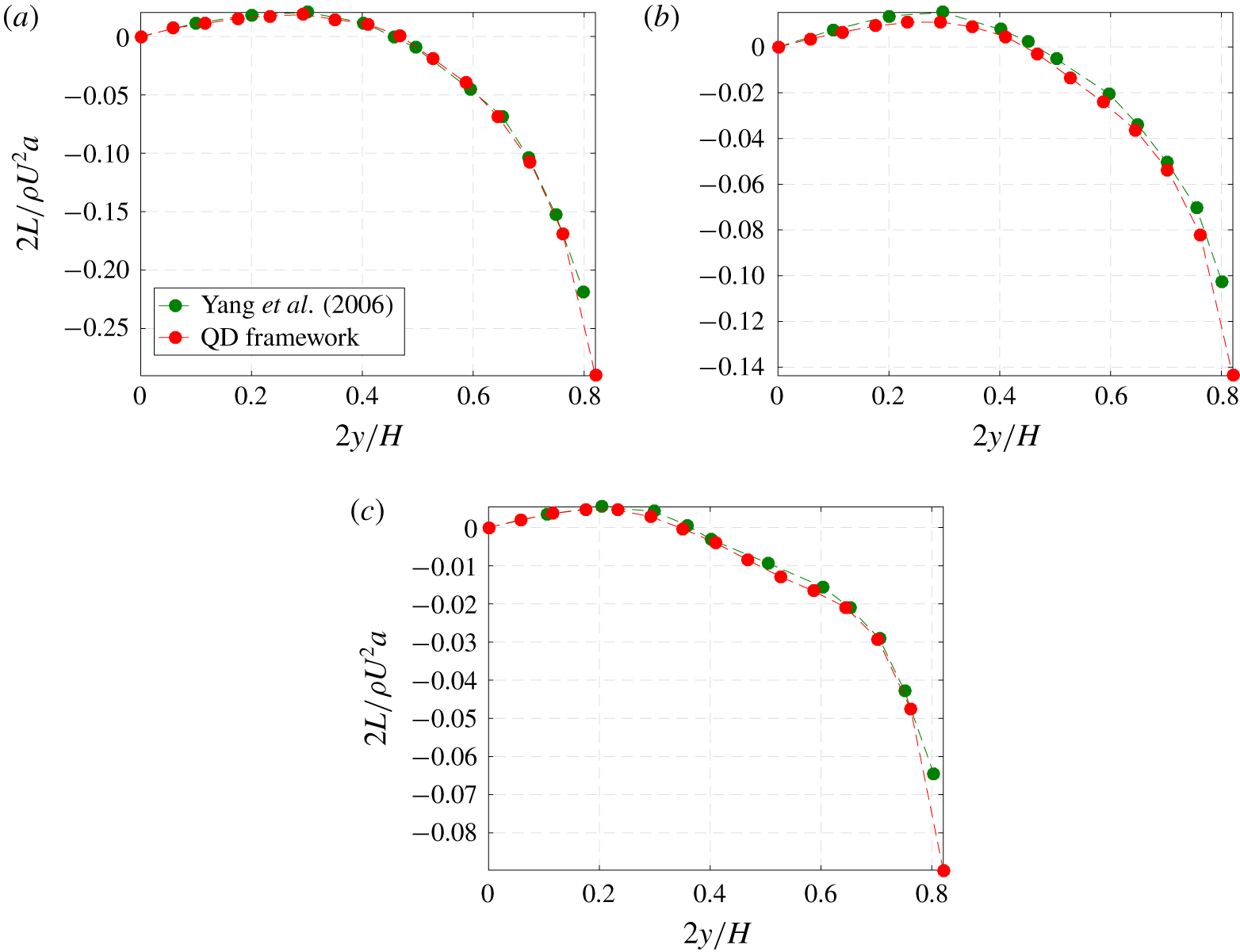
Validation for QD: lift variation in half-channel for  $k=0.15$ at
 $Re_{p}=$ (a) 1.667; (b) 15; and (c) 37.5.

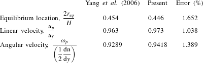
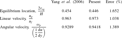
Equilibrium values for  $Re_{p}=15$ (
 $r_{eq},u_{p},u_{f},\unicode[STIX]{x1D714}_{p},\text{d}u/\text{d}y$ denote, respectively, stable location, particle linear velocity, undisturbed fluid velocity at centroid height of particle, angular velocity of particle and velocity gradient at particle centroid).
Declaration of interests
The authors report no conflict of interest.
Supplementary movies
Supplementary movies are available at https://doi.org/10.1017/jfm.2019.1007.
Appendix A. Validation
A.1 Circular particle in plane Poiseuille flow
The QD framework is validated by simulating the Segre–Silberberg effect (Segre & Silberberg Reference Segre and Silberberg1961) in two dimensions (Yang et al. Reference Yang, Wang, Joseph, Hu, Pan, Glowinski, Balachandar and Prosperetti2006). Fifteen particle locations are chosen in the radial direction, and particle Reynolds numbers of 1.67, 15 and 37.5 are used, where  $k=0.15$. The results are shown in figure 13, and are in excellent agreement with previous reports, including particle equilibrium locations, and velocities (table 2).
A.2 Elliptical particle in channel flow/sedimentation
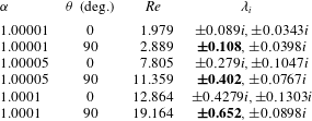
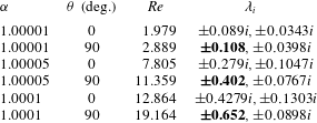
The ability of the approach to identify stable/unstable behaviour of non-circular particles is illustrated here. Specifically, we check for stability of elliptical particles in channel flow and find that there are no stable locations, which matches the behaviour observed with full FSI (tumbling  $+$ lateral bobbing) (Wen et al. Reference Wen, Chen, Qin, He and Zhang2016). We pick
 $k=0.3,Re=15$ for this configuration with a 1 : 2 ellipse aspect ratio. The eigenvalues for equilibrium at centreline (table 3) indicate instability, which agrees with the literature. Additionally, we validate against another case of a 1 : 2 elliptical particle settling under gravity for
 $Re>1$. The density difference (
 $\unicode[STIX]{x1D6FC}$) is controlled so that
 $Re$ at equilibrium does not exceed the limit beyond which fluttering occurs. The eigenvalues for this particle (table 4) at two orientations indicate stability with the major axis perpendicular to the settling direction, which agrees with the behaviour reported by Feng, Hu & Joseph (Reference Feng, Hu and Joseph1994).
Eigenvalues for elliptical particle in channel flow at centreline for two ( $XZ$) symmetric orientations (bold values correspond to unstable orientations).

Eigenvalues for sedimenting elliptical particle at centreline for two ( $XY$) symmetric orientations (flow direction along
 $Y$; values in bold indicate unstable orientations).
Appendix B. Damping-coefficient calculation
If  $\unicode[STIX]{x1D6FC}_{c}$ is the damping coefficient,
 $L_{c}$ is the restoring lift at the stable location and
 $m_{c}$ is the mass of the circular cylinder, then the equation of motion in the
 $y$-direction is
 $$\begin{eqnarray}m_{c}\frac{\text{d}^{2}y}{\text{d}t^{2}}=L_{c}(\,y)-\unicode[STIX]{x1D6FC}_{c}\frac{\text{d}y}{\text{d}t}\quad (\unicode[STIX]{x1D6FC}_{c}>0).\end{eqnarray}$$
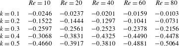
Assuming a linear variation of the position-dependent lift close to the stable point,  $L_{c}(\,y)=(\text{d}L_{c}/\text{d}y)y$, and drawing from the traditional spring–mass–damper system, the condition for under-damped motion for (B 1) becomes
 $$\begin{eqnarray}\displaystyle & \displaystyle \left(\frac{\unicode[STIX]{x1D6FC}_{c}}{m_{c}}\right)^{2}+\frac{4}{m_{c}}\frac{\text{d}L}{\text{d}y}<0, & \displaystyle\end{eqnarray}$$
 $$\begin{eqnarray}\displaystyle & \displaystyle \frac{\text{d}L}{\text{d}y}<0\;\Longrightarrow \;-2\sqrt{m_{c}\left|\frac{\text{d}L}{\text{d}y}\right|}<\unicode[STIX]{x1D6FC}_{c}<2\sqrt{m_{c}\left|\frac{\text{d}L}{\text{d}y}\right|}, & \displaystyle\end{eqnarray}$$
 $$\begin{eqnarray}\displaystyle & \displaystyle \unicode[STIX]{x1D6FC}_{c}>0\;\Longrightarrow \;0<\unicode[STIX]{x1D6FC}_{c}<2\sqrt{m_{c}\left|\frac{\text{d}L}{\text{d}y}\right|}. & \displaystyle\end{eqnarray}$$
Since we would like to use the damping coefficient as an estimate in the order-of-magnitude sense, any value in the above range should appropriately capture variations in damping with varying particle shapes and sizes, true to a given configuration and flow parameters. The damping coefficient of any arbitrary shape,  $\unicode[STIX]{x1D6FC}$, is then computed as
 $$\begin{eqnarray}\left.\begin{array}{@{}c@{}}\unicode[STIX]{x1D6FC}=\displaystyle \frac{K_{s}d_{v,s}}{K_{c}d_{v,c}}\unicode[STIX]{x1D6FC}_{c},\\ \text{where}\,\unicode[STIX]{x1D6FC}_{c}=\sqrt{m_{c}\left|\displaystyle \frac{\text{d}L}{\text{d}y}\right|}.\end{array}\right\}\end{eqnarray}$$
The ‘ $s$’ subscripts in equation (B 5) refer to the non-circular particle, and the ‘
 $c$’ refers to quantities pertinent to the circular particle. The parameters
 $K$ and
 $d_{v}$ stand for the dynamic shape factor, and volume-equivalent diameter, as defined in Leith (Reference Leith1987). The
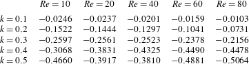
 $\text{d}L/\text{d}y$ term is computed using the non-dimensional counterparts from table 5.
Non-dimensional lift gradients,  $\text{d}L^{\ast }/\text{d}y^{\ast }$, evaluated for a circular particle at the stable equilibrium point, at select confinements,
 $k$, and Reynolds numbers,
 $Re$ (the negative sign indicates a restoring lift) – used for computing damping coefficients of non-circular shapes by means of a dynamic-shape factor (Leith Reference Leith1987).
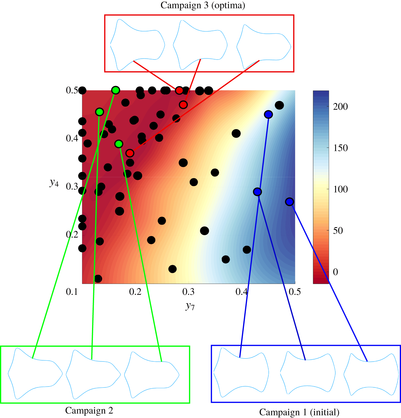
Two-variable optimization: optimization of  $y_{4}$ and
 $y_{7}$. Each dot represents a function evaluation using adaptive sampling via Bayesian optimization (60 function evaluations), while the underlying contour represents the original cost function surface (400 uniformly distributed function evaluations). Particle shapes corresponding to selected sampling locations are shown (colour coded).

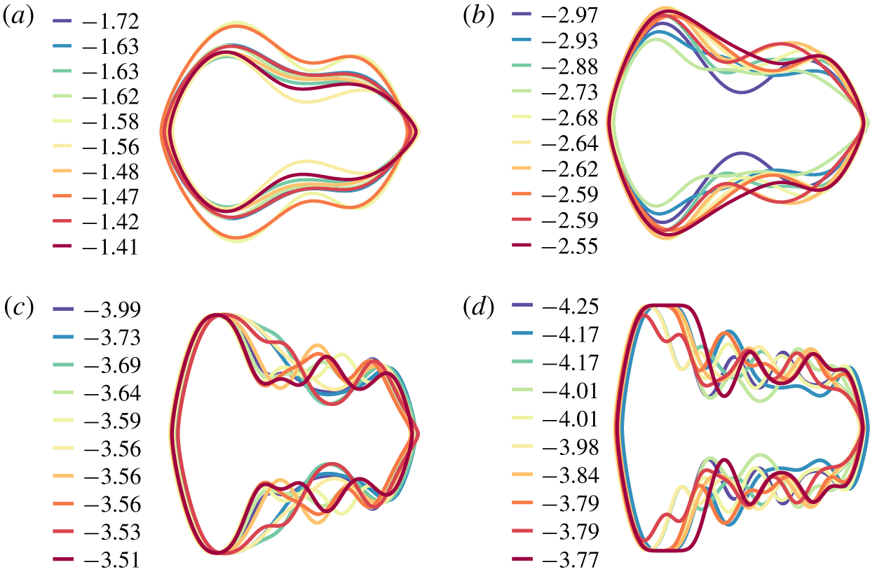
Best shapes without regularization: with ‘nv’ = (a) 4; (b) 6; (c) 10; and (d) 14 (the legend indicates normalized maximum of eigenvalue real parts ( $\unicode[STIX]{x1D706}_{max}/kRe$) – larger absolute values mean higher stability).

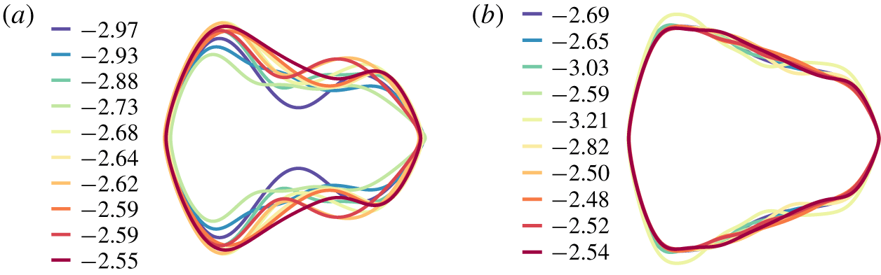
Best shapes with scaled-curvature penalty: (a) ‘nv’ = 6 without regularization; (b) ‘nv’ = 10 with regularization (the legend indicates normalized maximum of eigenvalue real parts ( $\unicode[STIX]{x1D706}_{max}/kRe$) – larger absolute values mean higher stability).

Appendix C. Optimization
We formulate the minimization as a fixed-budget problem as limited by the computational resources available. For each optimization run, we add as many infills (locations where the true function is evaluated each iteration as deemed ‘optimal’ according to the infill criterion) as it takes to arrive at a converged minimum (informed by previous optimizations performed on the original cost function using evolutionary algorithms). The first test is performed on a two-variable problem, where every candidate shape is defined by eight control points in total, with all but two of the control points fixed. Specifically, the variables  $y_{4}$, and
 $y_{7}$ from figure 1 are chosen to vary. Figure 14 illustrates the original function surface which is created using a
 $20\times 20$ mesh grid of the variables. It is seen that the reconstructions, which required a total of 60 function evaluations, are remarkably similar to the original function surface, which required 400 points. The metamodel is able to demarcate the stable and unstable regions of the original function reasonably well. Additionally, the infill criterion appears well calibrated as indicated by clustering of infill locations towards the minimum regions of the function, and a sparse set farther away. Moreover, this resolution of the optimal regions is conducive to the design problem, where we are interested in fully resolving the optima. Additionally, we use 2:1 infill-to-initial sampling, and 10 initial points per dimension (rule of thumb (Forrester, Sobester & Keane Reference Forrester, Sobester and Keane2008) for this test), which seems reasonable from findings. Our second test comprises a higher-dimensional optimization (
 $nv=6$). Contrary to the two-variable case, we run infill-to-initial ratios of 2, 5 and 10, and examine the range of fitness for the stable shapes. We find that higher stability is only achieved for an infill-to-initial ratio of 10, which closely matches our benchmarks from the genetic algorithm. Although the absolute difference in the best-fit values between ratios of 5 and 10 is approximately 16 %, we choose a ratio of 10 for all further runs due to the scope of improvement seen here.
Appendix D. Convergence in control points: $k=0.2$, $Re=20$


We run design optimization for the following tests:
(i) with 4, 6, 10 and 14 variable parametrization – without curvature-penalty regularization;
(ii) with 6 (without regularization) and, 10 variable parametrization (with scaled curvature penalty);
(iii) with 6 and 10 variable parametrization – both with log-curvature penalty.
For the first case (figure 15), it is seen that the best stability values increase with the number of control points due to the fact that the shape representation now allows for the introduction of crucial features which enhance particle stabilization. However, it is seen that the average trend of the shapes remains similar – fore–aft asymmetry characterized by a major aft segment with one or more smaller fore segments. But for ‘nv’ = 10, 14 (figure 15c,d), the shapes contain a significant number of small-scale features/bends which are undesirable. For the second case (figure 16), the cost function ( $C^{\ast }$) for a candidate shape is evaluated using the stability (
 $C$) and a scaled curvature integral (regularization) over the shape
 $$\begin{eqnarray}C^{\ast }=C+\unicode[STIX]{x1D6FC}\int _{S}^{}\unicode[STIX]{x1D705}^{2}\text{d}s,\end{eqnarray}$$
where  $\unicode[STIX]{x1D705}$ is the curvature at a segment of length,
 $\text{d}s$, on the shape;
 $\unicode[STIX]{x1D6FC}=0.1$ (configuration dependent) is chosen to offset the large variations in curvature with moderate changes in shapes, so as to not discard potentially stable shapes. The penalized shapes have fitness values which are quite similar to the shapes with the unregularized cost function, and also similar profiles to a certain extent. This essentially suggests that we can do away with the higher-‘
 $nv$’ parametrization with regularization by using ‘nv’ = 6, without the added dimensionality. However, it appears that the regularization used for the second case penalizes candidate shapes drastically, due to which we also investigate a log-curvature-integral regularization to reduce the effect of the penalty
 $$\begin{eqnarray}C^{\ast }=C+\log _{10}\left(\int _{S}^{}\unicode[STIX]{x1D705}^{2}\text{d}s\right).\end{eqnarray}$$
For the third case (see figure 17), we again see that although both ‘ $nv$ values produce different profiles, the stability values are close, which confirms that lower ‘
 $nv$’ without penalty would produce shapes of stability similar to those of a higher ‘
 $nv$’ with regularization. Thus, ‘nv’ = 6 is used for all further optimization runs.
Best shapes with log-curvature penalty: (a) ‘nv’ = 6; (b) ‘nv’ = 10 (the legend indicates normalized maximum of eigenvalue real parts ( $\unicode[STIX]{x1D706}_{max}/kRe$) – larger absolute values mean higher stability).

Appendix E. Fluid–structure interaction problem set-up
The transient simulations for designed particles are performed using ANSYS Fluent 18.1. The Dynamic-Mesh feature is utilized to account for changing particle boundary ( $\unicode[STIX]{x1D6E4}_{p}$) location every time step, using a boundary-fitted mesh. The fluid-flow equations are solved dimensionally using a finite-volume approach, and the particle positions and velocities are computed using the 6 degree-of-freedom rigid body solver, and updated using a multi-step predictor–corrector scheme. The particle chord length (‘
 $a$’) is always taken to be 0.1 m, and the fluid density and viscosity are taken to be
 $1000~\text{kg}~\text{m}^{-3}$ and 25 Pa s. We use no-slip walls (zero velocity), fully developed inlet and zero-pressure outlet boundary conditions. The initial conditions are set to be fully developed velocity and pressure fields throughout the channel, and the particle is released at rest, at a prescribed perturbation. The mesh close to the particle surface is refined sufficiently to preserve the particle shape as it deforms. Fluent uses a dynamic meshing method to account for the moving particle boundary with a boundary-fitted mesh that is updated according as the particle displacements – spring-based smoothing is performed as the mesh is updated; beyond a certain distortion, local cell remeshing is performed and flow fields are interpolated from the old mesh to the new mesh. The time step
 $\unicode[STIX]{x0394}t$ is limited as
 $\unicode[STIX]{x0394}t\leqslant \unicode[STIX]{x0394}x_{min}/2U_{max}$, where
 $x_{min}$ is the refined mesh size on the particle, and
 $U_{max}$ is the maximum fluid velocity. This condition ensures that the particle does not ‘crash’ into the mesh within one time step and invalidate it (negative volumes). Furthermore, an implicit mesh update during each time step is employed for additional stability. The particle is taken to be neutrally buoyant and the mass and moment properties are externally supplied through a user-defined function, which is invoked by the solver concurrently during runtime. A neighbourhood around the deforming zone is locally remeshed every few time steps to ensure a minimum quality of elements based on skewness, for accurate interpolation of flow fields from previous time steps.
We perform validation using three cases as detailed below.
E.1 Circular particle focusing in a straight channel
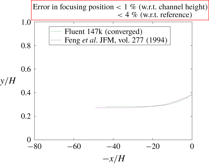
A circular particle focusing in planar Poiseuille flow is simulated. A circular particle is released in the bottom half of the channel with zero initial velocity, and initial condition for fluid is fully developed. The particles are neutrally buoyant. Far downstream, particles are expected to migrate to a constant lateral location. Channel width-to-length is 1 : 50,  $k=4$ and
 $Re=40$, referring to channel width and maximum fluid velocity. Spatial and temporal convergence is deferred to § E.4 below, and the trajectory for the converged case is shown in figure 18. The trajectories show an excellent comparison to literature with difference in focusing positions
 ${<}1\,\%$ relative to channel height.
Particle trajectories (Fluent with 147 k elements and reference).

E.2 Circular particle flowing around pillar in a straight channel
This application is of interest in the microfluidics community and has been previously reported by Xu et al. (Reference Xu, Xu, Kommajosula, Hsu and Ganapathysubramanian2019). An in-house finite element based framework employing a (moving) immersed boundary method (validated with sedimenting ball experiments) was used to simulate and compare with Fluent, and the results were in close agreement with each other. For the sake of brevity, the authors do not reproduce the details here and would like to refer the reader to the above reference for trajectories, velocities, set-up, etc. This is a case of complex geometries that Fluent is able to predict well.
E.3 Elliptical particle flowing in a straight channel
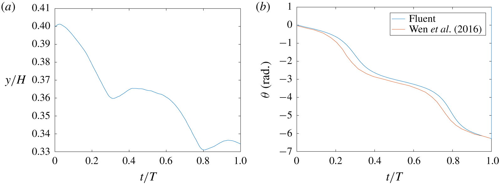
We simulate an elliptical particle of aspect ratio 1 : 2 released in a channel of aspect ratio 1 : 20, at  $Re=15$, based off of the channel width, and mean velocity. The particles are neutrally buoyant, and display similar behaviour as circular particles except that they bob and tumble about a constant mean lateral location far downstream. The set-up for this simulation is referenced from Wen et al. (Reference Wen, Chen, Qin, He and Zhang2016), and mesh density and time step are again taken from the converged case of § E.4. The evolution of the particle’s angle from the horizontal is plotted with time in figure 19. It can be clearly seen from figure 19(b) that the particle tumbles as expected, and is close in comparison with the literature.
(a) Lateral location with time, (b) orientation with time (Fluent and reference; ‘T’ refers to one time period of rotation).

In conclusion, the dynamic mesh method in Fluent is general and applicable to complex/non-circular particles as the particle geometry is accounted for in the unstructured remeshing algorithm itself, and the mass properties are supplied to the solver externally so the algorithm is not tailored for circular boundaries only.
E.4 Mesh and temporal convergence
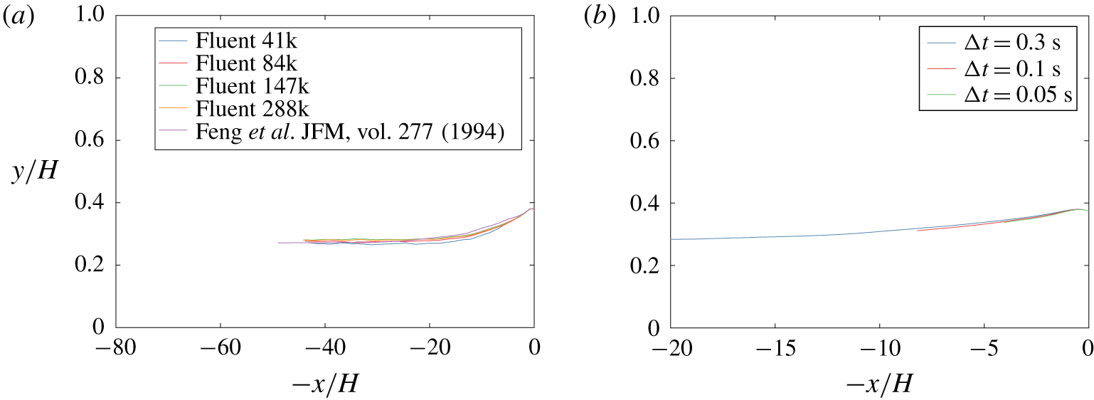
A circular particle focusing in straight channel flow is utilized to check spatial and temporal convergence in the FSI set-up; the parameters are the same as in § E.1 above. Mesh sizes of 41 000, 84 000, 147 000 and 288 000 elements were employed for the spatial convergence for time step 0.3 s (figure 20a). Although all trajectories are close to the reference, the trajectories start converging at 147 000 elements. The same is used for the time-step convergence (figure 20b), where it is seen that the trajectories are similar ( ${<}1\,\%$ difference) for
 $\unicode[STIX]{x0394}t=0.3~\text{s},0.1~\text{s}$ and
 $0.05~\text{s}$, and
 $\unicode[STIX]{x0394}t_{max}=\unicode[STIX]{x0394}x_{min}/2U_{max}$, as mentioned in appendix E above. These parameters are used for FSI simulations in the design validations.
(a) Spatial convergence, (b) temporal convergence (147 000 elements).