1. Introduction
What is the epistemic relation of present to past? Absent a time machine, we are trapped in the present and must rely on present traces to learn about the past. There are memory traces inside the skull, but outside there are tree rings, fossils, and traces of other kinds. People use these traces to reconstruct the past. Sometimes they simply assume that the traces provide unerring information about the past, but often they realize that the jump from present to past is subject to error. A bevy of epistemic concepts can be pressed into service to investigate the relation of present traces to past events, ranging from strong concepts like knowledge and certainty to more modest ones like justified belief and evidence.
We are interested in how the natural processes connecting past to present constrain our ability to know about the past by looking at the traces found in the present. An optimistic view of these processes is that the past is potentially an open book; all we need do is understand the connecting processes correctly and look around for the right traces. If the relation of the past state of a system to its present state were deterministic and one to one, this optimistic view would be correct. If only we could know the present state with sufficient precision, and if only we could grasp the true mapping function that connects present and past, we would be home free. This optimism is something that Laplace (Reference Laplace, Truscott and Emory1814, 4) affirmed when he discussed une intelligence (now referred to as “a demon”):
We may regard the present state of the universe as the effect of its past and the cause of its future. An intellect which at a certain moment would know all forces that set nature in motion, and all positions of all items of which nature is composed, if this intellect were also vast enough to submit these data to analysis, it would embrace in a single formula the movements of the greatest bodies of the universe and those of the tiniest atom; for such an intellect nothing would be uncertain and the future just like the past would be present before its eyes.
It is worth noting that determinism is not sufficient for the optimistic view to be true; without the one-to-one assumption, distinct states of the past may map onto the same state of the present, with the consequence that the exact state of the past cannot be retrieved from even a perfectly precise grasp of the present.
Is determinism necessary for the optimistic view to be true? It is not, provided that we set to one side strong concepts like knowledge and certainty and take up an epistemic evaluation that is more modest. Consider, for example, a process in which the system is, at each moment, in one of two states (coded 0 and 1). Suppose Past = 0 makes Present = 0 extremely probable (say, 0.96) and that Past = 1 makes Present = 1 extremely probable as well (say, 0.98). This means that when we observe the system’s present state, we gain strong evidence that discriminates between the two hypotheses Past = 0 and Past = 1. We cannot infer from Present = 0 that the past state was certainly 0; in fact, we cannot even infer that the past state was probably 0. But we can conclude that the observation favors the hypothesis that Past = 0 over the hypothesis that Past = 1. This conclusion is licensed by what Hacking (Reference Hacking1965, 59–62) calls the Law of Likelihood:
Observation O favors hypothesis H 1 over hypothesis H 2 if and only if  .
Royall (1997, 9–11) suggests that this qualitative principle should be supplemented by a quantitative measure of favoring:
The degree to which O favours H 1 over H 2 is given by the likelihood ratio  .
Royall further suggests that a reasonable convention for separating strong evidence from weak is a ratio of 8. Royall’s suggestion entails that the probabilistic process just described has the consequence that Present = 0 provides strong evidence favoring Past = 0 over Past = 1, since the likelihood ratio is 0.96/0.02 = 48.
This simple example should not be overinterpreted. If there were a process connecting past to present in the way described, the present would provide strong evidence about the past. Do not forget the if. Perhaps there are such processes, especially when the past under discussion is the recent past. But what if we consider not just the recent past, but past times that are more and more ancient? How does increasing the temporal separation between present and past affect the amount of information that the present provides about the past?
2. Two Theorems
A simple theorem provides an answer to the question just posed (Cover and Thomas Reference Cover and Thomas2006). Consider a system that at any time is in one of n possible states (s 1, s 2, …, sn). For simplicity we shall think of the system as evolving in discrete time steps. We stipulate that the system has the following two properties:
The Markov property. For any two times t 1 < t 2, the state of the system at time t 1 screens-off the system’s history prior to t 1 from the state at t 2. That is, for all states x and y:

Note that the Markov property does not require that the transition probabilities are constant with time (often called ‘time-homogeneous’ chains); rather, they may vary from step to step.
The second property we stipulate is sometimes referred to, in the time-homogeneous, finite-state setting, as the Markov chain’s being “regular”; we will use the same term in the broader setting we are considering in which time homogeneity is relaxed:
Regularity. For some positive integer n, and some strictly positive real value ε, the following holds for all ordered pairs of states (i, j): given that the system at any given time t is in state i, the probability that the system is in state j at time t + n is at least ε.
This condition asserts that it is possible to move from any given state to any other state (including the original state) in a fixed finite number of steps with a probability that remains bounded above zero. Regularity for finite-state time-homogeneous Markov processes is equivalent to the condition that the Markov chain is ‘aperiodic’ and ‘irreducible’ (for details, see Häggström [Reference Häggström2002, corollary 4.1]).
For any system of this sort, the following result holds (a precise statement and proof is provided in app. A):
Exponential information loss theorem. If a finite-state system satisfies the Markov property and regularity, then I(Past; Present) is less than or equal to a term that approaches zero exponentially fast as the time between the present and past increases.
Here I(X; Y) is the “mutual information” linking the two variables. If the variables are discrete, the formula for this quantity is

where p(x, y) is the joint probability that X = x and Y = y, and p(x), p(y) are the (marginal) probabilities that X = x, and that Y = y, respectively. Mutual information measures how much (on average) you learn about the state of one of the variables by observing the state of the other. Its value is zero when X and Y are independent; otherwise it is positive. Mutual information is symmetrical: I(X; Y) = I(Y; X).
The exponential information loss theorem generalizes the special case where transition probabilities are constant with time (Sober and Steel Reference Sober and Steel2011, proposition 6). This generalization is important, since many processes (including the biological examples we will discuss) often change their rates from one period of time to another.
Note that the theorem does not ensure a monotonic decline in information as the temporal separation of past and present is increased. That extra element is provided by a different result, the so-called Data Processing Inequality (DPI; Cover and Thomas Reference Cover and Thomas2006, 32):
The Data Processing Inequality: In a causal chain from a distal cause D to a proximate cause P to an effect E, if P screens-off D from E, then I(E; D) is less than or equal to both I(E; P) and I(P; D).
For a discrete-state process, these two inequalities are strict whenever P is neither perfectly correlated with D or with E, nor is P independent of them (see app. B). The Data Processing Inequality does not require that the process linking D to P is the same as the process linking P to E.
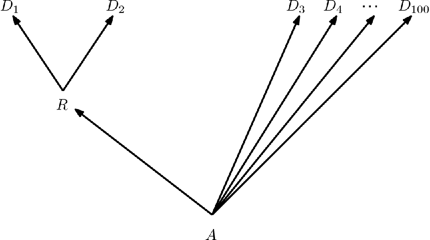
The information-processing inequality is “chain internal.” It does not say that the present always provides more information about recent events than about ones that are older. Consider figure 1. Suppose that R screens-off A from D 1 & D 2 Then the information-processing inequality says that  . It does not say that
 . It is perfectly possible that the hundred descendants that now exist provide more information about A than they do about R. Note that R does not screen-off A from D 1 & D 2 & … & D 100. The heightened information that the leaves provide about A is not due to the simple fact that A has a larger number of outgoing lineages than R does; it is possible to modify this tree so that each nonleaf node (including the root node A) has just two descending lineages (Sober and Steel Reference Sober and Steel2011, fig. 5b, 243–34), and still the leaves provide more information about A than they do about R, owing to the values of the transition probabilities attaching to branches.
A case in which it is possible for the present to provide more information about an ancient event (A) than about a more recent event (R).

Both the exponential information loss theorem and the Data Processing Inequality are very general. They characterize any system whose laws of motion have the requisite probabilistic features. The system might be a chamber of gas, but it also might be an evolving population of organisms. Indeed, if there were disembodied spirits that changed probabilistically, the results would apply to them. Both results are more general than physics—they cover the systems and properties that are discussed in the laws of physics, but they also apply to systems and properties that are not. In addition, both results are a priori mathematical truths, although of course it is an empirical matter whether a given system satisfies the antecedent of the conditional that each result expresses (Sober Reference Sober2011a).
3. Five Evolutionary Processes
Since our interest here is in how evolutionary processes affect the amount of information that the present provides about the past, it is worth making clear how the exponential information loss theorem applies to models of biological evolution. In phylogenetics, the rapid loss of information in models of nucleotide substitution with time has been highlighted as a significant problem for using DNA sequence data to accurately resolve deep divergences of species lineages (for a recent review, see Salichos and Rokas [Reference Salichos and Rokas2013]) and for inferring ancestral states deep within a given tree (Mossel Reference Mossel2003; Gascuel and Steel Reference Gascuel and Steel2014).
We will return to phylogenies in a later section, but for now we consider information loss in population genetics. The application of information theory to population genetics has been investigated a bit. For example, Frieden, Plastino, and Soffer (Reference Frieden, Plastino and Soffer2001) explore a variational principle (“extreme physical information”) based on Fisher information to study genotype frequency changes. The questions we consider here are different, as our primary interest is in the relative ranking of likelihood ratios across different evolutionary processes, including both drift and different types of selection. The Moran (Reference Moran1962) models of evolution will be our workhorse in what follows. We consider a population containing N individuals. The population evolves through a sequence of discrete temporal “moments” (how long a moment is will not matter). At each moment, one of those N individuals produces a copy of itself and one of those N individuals dies. We consider two traits A and B; each individual has one of them or the other. At any moment, the population is in one of N + 1 states (ranging from 0% A to 100% A). This Moran framework can be articulated in different ways to represent different evolutionary processes. For example, if individuals are chosen at random to reproduce and die, then we have a drift process. Selection processes of different kinds can be represented by letting A individuals have chances of dying or reproducing that differ from those possessed by B individuals. A population undergoing a Moran process forms a Markov chain, with its recent past screening-off its more remote past from the present.
Suppose we observe the population in the present and see that all N individuals are in state A. How much information does that observation provide about the state of the population at some earlier time? If all states are accessible to each other (which requires that mutations can prevent the population from getting “stuck” at 100% A or 100% B), then the exponential information loss theorem applies and so the mutual information declines asymptotically to zero with time. However, if there is no mutation, then the population will evolve to either 100% A or 100% B and will stay there. In this case, the present state of the population provides information about its past even if the two are infinitely separated. For example, if we observe that the population is now 100% A and the population has been evolving by drift, this observation favors the hypothesis that the population was at more than 95% A at some earlier time over the hypothesis that it was 5% A or less, and this is true regardless of the time separation between the past and the present.
John Maynard Keynes (Reference Keynes1924, chap. 3) once said that “in the long run, we are all dead.” His point was to pooh-pooh the relevance of claims about the infinite long run. What should matter to us mortals is finite time. This point applies to the bearing of the exponential information loss theorem on our knowledge of the evolutionary past. Who cares if mutual information goes to zero as the time separating present from past goes to infinity? Life on earth is a mere 3.8 billion years old. What is relevant is that information decays monotonically in Markov chains. But in addition, we know that there are different kinds of evolutionary process. Which of these speeds the loss of information and which slows it?
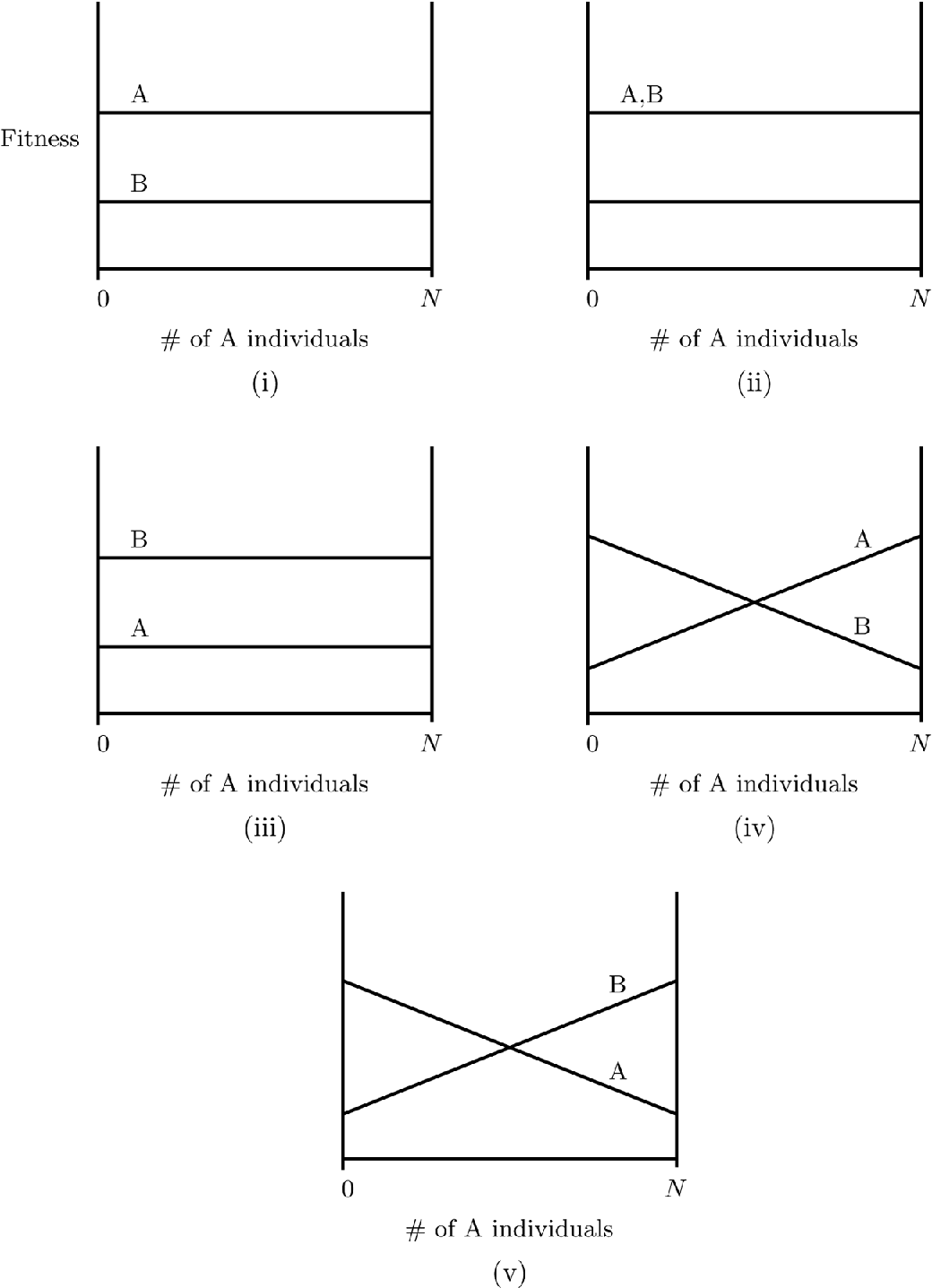
The five processes we want to investigate are represented in figure 2; each of them can result in our present observation that all N of the individuals in the population now have trait A. In panel i, trait A was favored by selection. In panel iii, there was selection against trait A. In panel ii, the traits are equal in fitness, and so the traits evolved by pure drift. In panel iv, selection favored the majority trait. And in panel v, selection favored the minority trait. We are not asking which of these process hypotheses is most plausible, given the observed state of the population at present. Rather, we want to explore what happens to information loss under each of these five scenarios, in each case thinking of the process in the context of the Moran framework of a finite population of fixed size N.
Five processes that can result in all N of the individuals now in the population having trait A.

To compare the five processes in this respect, we calculate the following likelihood ratio for each of them:

Although our main interest is to compare cases in which i is close to N and j is close to 0, the Moran framework makes it easy to derive results for the more general case in which i > j.
So the observation is that all N of the individuals now in the population have trait A. Does this observation favor the hypothesis that there were exactly i individuals at some past time who had trait A over the hypothesis that there were exactly j, where i > j? It does; Rij > 1 for each of the five processes we are considering (see app. C). Our question is how the magnitude of Rij depends on the underlying evolutionary process. It is worth noting that although the likelihood ratio Rij is “past-directed” (in that it describes the degree to which a present observation discriminates between two hypotheses about the past), evaluating this ratio requires one to consider two “future-directed” probabilities—the probability of reaching Present = N if the system begins at Past = i and the probability of reaching Present = N if the system begins at Past = j.
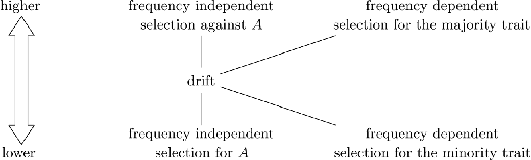
We begin by adopting an assumption that we treated above with Keynesian disdain. Let us assume that the temporal separation of past and present is infinite and that there is zero mutation. We will relax this idealization in due course. For each of the processes we are considering, we now can describe what the value of Rij is for each pair of values for i and j such that i > j. For example, under neutral evolution the value of R ij is i/j. The values for the other four processes are given in appendix C. The ordering of the Rij values for the five processes is depicted in figure 3.
Comparing Rij values for five processes, assuming infinite temporal separation of Past from Present and zero mutation. The relation of the two frequency-dependent processes to drift is derived using the assumption that j < N/2.

Let us first consider three of the cases described in figure 3—drift and the two cases of frequency-independent selection. The ordering of Rij values for these three processes means that the observation that all the individuals in the population now have trait A provides more information about the past state of the population the less probable it was that A would evolve to fixation. Selection for A is at the bottom of the pile, with neutrality next, and selection against A at the top.
The ordering of these three processes has an intuitive interpretation. Suppose we observe that trait A is fixed in a population and we wish to estimate whether A was common (at frequency i) or rare (at frequency j < i) at some time in the past. Selection for A makes it easy for A to go to 100% in the population, regardless of whether it starts off common or starts off rare, which is why selection for A comes in last in the part of figure 3 that describes frequency-independent processes. The evidence in favor of the former hypothesis relative to the latter, as measured by the likelihood ratio, is stronger under selection against A than under a drift model. This is because the drift model provides more opportunity for a rare allele A to fix at 100% in the population than the model in which A is selected against. For a formal proof concerning how the Rij values for different processes compare, see appendix C.
The three results depicted in figure 3 that describe frequency-independent processes echo an insight that Darwin expresses in the Origin: “Adaptive characters, although of the utmost importance to the welfare of the being, are almost valueless to the systematist. For animals belonging to two most distinct lines of descent, may readily become adapted to similar conditions, and thus assume a close external resemblance; but such resemblances will not reveal—will rather tend to conceal their blood-relationship to their proper lines of descent” (Darwin Reference Darwin1859, 427). Darwin illustrates this idea by giving an example: whales and fish both have fins, but this is not strong evidence for their common ancestry, since the trait is an adaptation for swimming through water. Far stronger evidence for common ancestry is provided by similarities that are useless or deleterious. One of us has called this idea Darwin’s Principle, in view of its centrality to Darwin’s framework (Sober Reference Sober2008, Reference Sober2011b).
Darwin’s topic in the passage quoted is inferring common ancestry, not inferring the past state of a lineage from its present state, but the epistemologies are similar. Here is a simplified argument that illustrates why. Suppose trait A has probability p of being fixed in a recent species. If two species x and y diverged from their most recent common ancestor very recently, the probability that they both have trait A is approximately p. On the other hand, if they have no common ancestor, then the probability of them both having A is p 2. This means that the likelihood ratio of the hypotheses “x and y have a recent common ancestor” and “x and y have no common ancestor” is approximately p/p 2 = 1/p under Markovian trait evolution. Thus, the smaller p is, the greater this likelihood ratio will be. And the value for p if there is selection for A is larger than the value for p if there is drift, which in turn is larger than the value for p if there is selection against A.
There are two cases of frequency-dependent selection represented in figure 3. One of them (frequency-dependent selection for the majority trait) shows that it would be an overstatement to say that the current state of the population (all individuals having trait A) always provides scant evidence concerning the population’s past state if trait A evolved because of natural selection. It matters a great deal what sort of selection process we are talking about. Frequency-dependent selection for the majority trait is better than drift in terms of how much information the present state of a lineage provides about its past. Figure 3 also locates the evidential meaning of frequency-dependent selection for the minority trait; it has an informational yield that is worse than that provided by drift. As noted in appendix C, our results for both cases of frequency-dependent selection make the assumption that j < N/2. This assumption ensures that the ordering of the frequency-dependent selection cases is always maintained as shown in figure 3; it is an innocent assumption since, as noted above, we are mainly interested in the case where i and j are majority and minority values, respectively.Footnote 1
Figure 3 provides only a partial ordering of the five cases depicted. The reason for this is that a comparison of, say, frequency-independent selection against A with frequency-dependent selection for the majority trait would depend on the values of specific parameters.
We now can remove the idealization of infinite time and zero mutation. The ordering of the Rij ratios for the five processes, when time is infinite and mutation is zero, is the same as the ordering of those processes for the following slightly different likelihood ratio, when time is finite (and sufficiently large) and there is a sufficiently small mutational input:

See appendix D for a proof of this ordinal equivalence result. Here “Past ≈ N” and “Past ≈ 0” just mean any states close to N and to 0 (respectively), which are then held fixed across the five models. With mutational input, the exponential information loss theorem applies to all five processes. The mutual information between present and past declines monotonically as their temporal separation increases, but the decline is faster under some processes than it is under others.
Our results are derived within the setting of the Moran model of population genetics. This is a finite-state Markov chain that forms a “continuant process” (Ewens Reference Ewens2010). That is, at each step the number of individuals carrying a particular allele in the population of fixed size N either goes up by 1, or goes down by 1, or it stays the same. We expect similar conclusions concerning the partial ordering of the Rij ratios for other continuant processes, provided the transition probabilities faithfully reflect the various types of selection being compared. Our results also apply to a slightly different problem: how does the kind of evolutionary process at work in lineages affect the strength of the evidence that similarity provides for common ancestry (Sober Reference Sober2008)?
4. Mutual Information and the Likelihood Ratio
We began our discussion of information loss by using the concept of mutual information but then shifted to considering the likelihood ratio. Have we illicitly changed horses in midstream? We think not. Consider the mutual information between the binary random variable E that takes the value 1 if allele A is fixed in the present population (E = 0 otherwise), and the frequency X of allele A in the past population, under some strictly positive prior distribution. In this case, mutual information and the likelihood ratio are linked as follows:

If we now observe E = 1, then instead of comparing I(X; E) across the different processes, it is more relevant to compare the values of Rij. That is, we are thinking of a single observation (Present = N), so we are not considering all the possible observations that we might make of the present state. This is why we used the likelihood ratio Rij rather than mutual information to carry out the cross-process comparison.
5. The Impact of Branching on Information
We have emphasized that loss of information within a lineage is a fact of life. However, the branching that takes place in evolution is a force that pushes in the opposite direction, since it creates new lineages. As illustrated in figure 1, it is possible for an ancient ancestor to have more present-day descendants than a more recent ancestor has, and this means that the information lost to the passage of time can be offset by the proliferation of descendants that each bear witness to the ancient ancestor’s state. If the process is a symmetric one on two states, it is possible to describe precisely how often branching must occur if information loss is to be offset in this way (Evans et al. Reference Evans, Kenyon, Peres and Schulman2000); for more general processes, one must usually be content with upper and lower bounds.
It might be asked why one needs to worry about observing descendants to infer the characteristics of ancestors. Doesn’t observing fossils provide a simpler and more definitive solution? Our answer has three parts. First, one cannot assume that a fossil comes from an ancestor of extant species; it may just be an ancient relative. Second, fossils provide evidence about the morphological hard parts of ancient organisms; molecular characters, not to mention phenotypic features of physiology and behavior, typically do not fossilize. And finally, fossil traces degrade and are subject to the exponential information loss theorem if fossils change state in conformity with the regularity assumption and have the Markov property.
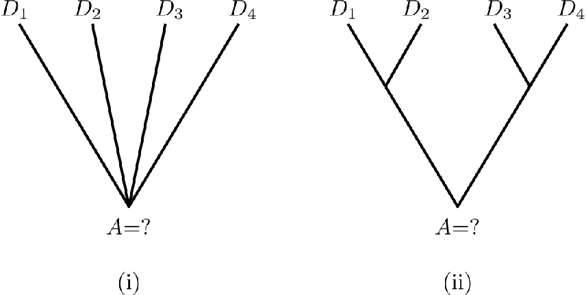
Just as the process at work in lineages has an impact on information loss, so too does the topology of the branching process itself. It might seem intuitive to conjecture that the star phylogeny shown in figure 4i is “better” than the bifurcating topology shown in figure 4ii in the sense that the former topology allows the observations to provide more information about the root than the latter topology does. In order to hold other factors fixed, we assume that the two topologies have the same number of leaves and that the process at work in branches is the same in the two topologies (in particular, that the expected number of substitutions—the branch lengths—between the root and each leaf match up for the two trees). The conjecture just stated seems reasonable, since in figure 4i the observations are independent of each other, conditional on the state of the root, whereas in 4ii, the observations are not conditionally independent. The guess is correct for a two-state symmetrical process when we compare the two trees in figure 4 (Sober Reference Sober1989, 280). More generally, this guess holds whenever we compare any binary tree with a matching star phylogeny on the same number of leaves when a two-state symmetric process is at work (Evans et al. Reference Evans, Kenyon, Peres and Schulman2000). But, surprisingly, the guess is not always true for symmetric Markov processes with more than two states.
Does observing the four leaves of the star phylogeny (i) provide more information about the state of the root than observing the four leaves of the bifurcating phylogeny (ii)?

More precisely, consider a completely balanced binary tree with 2n leaves, on which a constant symmetric process on five (or more) states operates with a constant substitution probability on each edge of the tree. Then if this substitution probability lies in a certain region, and n is large enough, the mutual information between the leaf states and the root state can be higher for the binary tree than for a comparable star tree on the same number of leaves (Sly Reference Sly2011, theorem 1.2). Here “comparable” means that the expected number of substitutions from the root to any tip is the same in both trees. In other words, the root state of a tree can sometimes be more accurately predicted from the state of its leaves when the tree is binary (and the leaves are correlated) than when the tree is a star (and the leaves are independent), where the two trees have the same marginal distribution. A similar result holds for strongly asymmetric two-state models (Mossel Reference Mossel2001, theorem 1). So the intuitive maxim that testimony from independent witnesses of an event provides more information about the event than testimony from otherwise similar dependent witnesses is sometimes false.
6. Conclusion
In summary, the view of evolution as an “information-destroying process” is basically right, but it overlooks some interesting details. For some special processes (e.g., zero mutation in simple population genetic models), information never completely disappears, even after infinite time. For example, under a drift model with zero mutation, some information concerning whether allele A was initially in the minority or the majority is always detectable at any time in the present frequency of A (which eventually fixes at 0 or N) in the population. At the other extreme there are certain (discrete time) processes for which the information can collapse completely to zero in finite time (Mossel Reference Mossel1998; Sober and Steel Reference Sober and Steel2011, 233).
The more usual situation lies between these two extremes; for processes that are Markovian and regular, the information between past and present decays at an exponential rate and vanishes only in the limit. Here we can still compare the relative support such models provide in estimating an ancestral state from an observation today. For the five models considered, this support varies in a predictable way depending on the type of model assumed.
We are well aware that the Moran framework contains various simplifications (e.g., constant population size), but the model’s simplicity allows for explicit calculations and results and does not raise questions as to whether the ordering might depend on the complexities that might be introduced in a more intricate model. We hope that our results will provide a foundation for exploring how adding complexities affects information loss. In philosophy as well as in science, it is reasonable to walk before one runs.
The estimation of an ancestral state from the leaves of a phylogenetic tree exhibits further subtleties, along with a surprise: the independent estimates obtained from a star phylogeny may or may not be more informative than the correlated estimates obtained from a binary tree, depending on the number of states, the size of the tree, and the substitution rate. The epistemological principle that “the testimony of independent witnesses always provides more evidence than the testimony of otherwise similar dependent witnesses” is wrong.
Appendix A: Formal Statement and Proof of the Exponential Loss Theorem
Proposition 1. Suppose X t; t ≥ 0 is any discrete, finite-state Markov process that satisfies the following condition. For some  , and integer N > 0 the following inequality holds for all t ≥ 0 and states i, j:

Then  for constants C, c > 0.
Proof. Let Yn be the ‘N-step’ Markov chain defined by Yn = XnN for all n ≥ 0. Note that equation (A1) implies that Yn satisfies the following inequality for all n, i, j:

We will show that

for constants B, b > 0, from which proposition 1 follows because if t = nN + r for 0 ≤ r < N then

where the first inequality is from the Data Processing Inequality, and the second inequality is from (A3). Thus we can take C = Beb, and c = b/N to obtain (A1) from (A2).
To establish inequality (A3) we apply a standard type of coupling argument. For k ≥ 0 let  for each state i. Consider the following Markov process
 defined as follows:
 and for each k ≥ 0, the state of
 is determined as follows: At each step of this chain, we toss a biased coin, which returns a head (H) with probability
 (independently of the chain) or a tail (
 ) with probability
 . If a head H is returned,
 is assigned a random state according to the distribution
 . If the coin toss results in a tail
 outcome, then
 selects a state that depends on
 as follows: if
 , then
 is assigned state j with probability

Note that this expression is greater than or equal to zero (by 2), and is less than or equal to 1; moreover,

so (A4) describes a legitimate probability distribution conditional on  .
By the law of total probability we can express  as follows:

Summarizing, we have:  , and
 , and so Yk and
 describe the same Markov chain. In particular,
 , and
 . Let

and let  be the event that H occurs at least once in the first n biased coin tosses that are performed in the construction of the chain
 . Then pn(i, j) can be written as the sum of two terms:

Now, the first term in (A5) is exactly  since
• conditional on
 , is independent of and, in addition, is distributed as πn; and
•
and are independent, and so
 ,
 is independent of
 and, in addition,
 is distributed as πn; and
 and
 are independent, and so

The second term in (A5) can be written as  multiplied by a term that lies between 0 and
 , since

Thus, selecting b > 0 so that  we can write:

where, as usual, ‘f (n) = O(g(n))’ is shorthand for the statement that f (n) is at most some constant times g(n). Finally, observe that, from (A2),  and so, from (A6):

for a constant B > 0. Since  , this establishes (A3), as required. QED
Appendix B
Proposition 2. Suppose that X → Y → Z forms a Markov chain, where the state spaces for X, Y, and Z are discrete, and  and
 for all choices of states x, y, z for X, Y, Z, respectively. Then the DPI is an equality if and only if X, Y, and Z are mutually independent.
Proof. First, observe that if X, Y, Z are independent then they are pairwise independent and so I(X; Y) = I(X; Z) = I(Y; Z) = 0 and thus equality holds trivially. Next, suppose that  for all choices of states x, y, z for X, Y, Z, respectively. Then
 holds also (since X → Y → Z is a Markov chain). Suppose further that the DPI is an equality; we will show that X, Y, and Z are independent. Since the DPI is an equality, X → Y → Z and X → Z → Y are both Markov chains (Cover and Thomas Reference Cover and Thomas2006). We write p(xyz) as shorthand for the probability
 and similarly for conditional and marginal probabilities (thus, e.g.,
 ). First observe that the positivity condition p(xyz) > 0 for all (x, y, z) implies that p(xy), p(xz), p(yz), p(x), p(y), p(z) are also strictly positive. Since X → Y → Z is a Markov chain, and p(xy) > 0:

and since X → Z → Y is also a Markov chain, and p(xz) > 0, we have p(xyz) = p(y|xz) p(xz) = p(y|z) p(xz). Applying Bayes’s theorem, the last term can be written as

(note that p(z) > 0) and so, combining this with equation (B1) gives

and so

Since p(z|y) > 0 (because p(yz) > 0) we can cancel this term on the left and right of equation (B2) to obtain:

Now, we can further write p(xy) = p(x|y) p(y) and p(xz) = p(x|z) p(z) which, upon substitution into equation (B3) gives:

in other words, p(x|y) = p(x|z) (noting that p(y), p(z) > 0). Now, this equation must hold for all choices of x, y, and z so p(x|y) must be constant as y varies—which implies that X and Y are independent. Similarly X and Z are independent. Finally, reversing the two Markov chains gives that Z is independent of Y. Thus X, Y and Z are pairwise independent.
Moreover they are independent as a triple since X → Y → Z is a Markov chain and so

QED
Appendix C: Rij Ratios with Zero Mutation at the Infinite Time Limit
Consider the Moran model in population genetics, with two trait values A and B and population size N. Let  be the number of copies of A in the population at time t. In this section we assume zero mutation, and we consider neutral evolution, selection for A, selection against A, and frequency-dependent selection (for the majority state and against the majority state). Since each of these Markov processes has absorbing states 0 and N (because of zero mutation) eventually one allele will be fixed and the other lost. Let
 be this end state, and
 the starting state (thus S = X 0 and
 ).
We are interested in comparing the ratio of conditional probabilities:

for i > j under the various models.
(i) Under neutral evolution
, for all 0 < i, j ≤ N.(ii) Under frequency-independent selection
, for all 0 < i, j ≤ N, where c is a positive constant with c < 1 when there is selection for A and c > 1 when there is selection against A.(iii) For any two values i, j ∈ {1, 2, … , N} with i > j the R ij value for selection against A exceeds the R ij value for neutral evolution, which in turn exceeds the R ij value for selection for A.
(iv) For frequency-dependent selection, where the fitness of trait A is proportional to its frequency, the associated R ij value exceeds that for neutral evolution for all i, j ∈ {1, 2, … , N} with i > j provided that j < N/2.
(v) For frequency-dependent selection, where the fitness of trait A is proportional to the frequency of the alternative trait B, the associated R ij value is lower than that for neutral evolution for all i, j ∈ {1, 2, … , N} with i > j, provided that j < N/2.
(vi) In all the cases considered above we have R ij > 1 for all i > j.
 , for all 0 < i, j ≤ N.
 , for all 0 < i, j ≤ N, where c is a positive constant with c < 1 when there is selection for A and c > 1 when there is selection against A.
Proof: Part i. For any integer x∶ 0 ≤ x ≤ N it is a well-known result (for many neutral models) that

(see, e.g., eq. 3.49 of Ewens Reference Ewens2010), from which i immediately follows.
Part ii. From Ewens (Reference Ewens2010, eq. 3.66) we have, for any x ∈ {1, … , N}:

for a positive constant c which is greater than 1 for selection against A and less than 1 for selection for A. Part ii now follows immediately.
Part iii. By parts i and ii, part iii is equivalent to the assertions that for i > j, if c ∈ (0, 1) then:

while if i > j and c > 1 then:

Now, using the identity 1 − ck = (1 − c) (1 + c + c 2 + … + ck −1) we have

and so we wish to compare

which is equivalent to comparing

Now, the left-hand side is merely the average of the terms ck from k = 0 up to k = i − 1 while the right-hand side is the average of these terms up to j − 1 and since i > j the left-hand side is smaller than the right when c < 1 and greater when c > 1. This completes the proof.
Part iv. When selection is frequency dependent, we need to use the expression:

where fk and gk denote the fitnesses of alleles A and B, respectively, when k individuals have allele type A (see, e.g., Huang and Traulsen Reference Huang and Traulsen2010, eq. 6). If we now take the fitness of trait A to be proportional to its frequency, that is fk = a · k for a constant a > 0, and take the fitness of trait B to also be proportional to its frequency (with the same coefficient)—that is, gk = a · (N − k)—then equation (C2) gives

As before, this ratio exceeds i/j precisely when the average of the first i terms

(for m = 0, 1, 2 …) exceeds the average of the first j terms

this holds for all i > j with j < N/2.
Part v. If we take the fitness of trait A to be proportional to the frequency of B, that is fk = a · (N − k) for a constant a > 0, and take the fitness of trait B to be proportional to the frequency of A (with the same coefficient)—that is, gk = a · k—then equation (C2) gives

and this ratio is lower than i/j precisely when the average of the first i terms

(for m = 0, 1, 2 …) is lower than the average of the first j terms

this holds for all i > j with j < N/2.
Part vi. The inequality Rij > 1 for i > j is trivial for neutral evolution, while for the other processes the inequality follows from equations (C1), (C3), and (C4), noting that when i > j the i terms in the numerator include the j terms in the denominator along with some additional positive terms.
Note that N plays no role in the expression of the ratio Rij in cases i–iii, but it does for iv and v.
Appendix D: Rij Ratios with Finite Time and Nonzero Mutation Rate
The results in the previous section assume zero mutation and consider the infinite time limit. However, they also have some bearing on what happens at finite time and for nonzero mutation. First assume zero mutation and consider the ratio Rij at finite times t. Since these ratios are continuous functions of t and converge to values that satisfy the partial order described in figure 3, this ordering also holds for t sufficiently large (but finite). Select any such sufficiently large value t 0 of t, and consider this ratio Rij at t 0 as a function of the mutation rates. Again, Rij is a continuous function of these mutation rates (with t fixed to t 0), and so, for sufficiently small (but nonzero) mutation rates, the five Rij values will still be ordered as in figure 3 at t 0. In summary, for a sufficiently large value of time, we can take small but strictly positive mutation rates that preserve the order of the Rij ratios shown in figure 3. This ordering may change if the mutation rates are then held fixed and time increased. In other words, the order of quantifiers here is important. We are merely asserting that for any sufficiently large value of time, there exist positive mutation rates that preserve the orderings of the ratios—if we select a larger time, the mutation rates may need to be reduced (but will still be strictly positive).