2 Details of the numerical simulations

We consider very small bubbles dispersed in an isotropic homogeneous turbulent flow. The continuous liquid phase is given by the incompressible Navier–Stokes equation and the dispersed phase is treated with a point particle approach. The feedback of the bubbles on the carrier phase is disregarded. The carrier flow field is computed with a pseudo-spectral method in a periodic box (Zamansky et al. Reference Zamansky, Coletti, Massot and Mani2016; Gorokhovski & Zamansky Reference Gorokhovski and Zamansky2018; Bos & Zamansky Reference Bos and Zamansky2019). In order to maintain a statistically stationary state, a forcing term active at the smallest wavenumbers is applied to the Navier–Stokes equation (Chen et al. Reference Chen, Doolen, Kraichnan and She1993). The flow field is simulated by DNS and LES for the same Reynolds number, and the details of the simulation parameters are given in table 1. For the LES, the turbulent viscosity is estimated by the standard Smagorinsky model, $\unicode[STIX]{x1D708}_{\unicode[STIX]{x1D6E5}}=C_{s}\unicode[STIX]{x1D6E5}|\overline{\unicode[STIX]{x1D61A}_{ij}}|$ , where $\overline{\unicode[STIX]{x1D61A}_{ij}}$ is the filtered rate of strain tensor, $\unicode[STIX]{x1D6E5}$ is the cutoff scale and $C_{s}$ is the model parameter. With the Smagorinsky model, the energy transfer rate from scale $\unicode[STIX]{x1D6E5}$ , $\unicode[STIX]{x1D700}_{\unicode[STIX]{x1D6E5}}=2(\unicode[STIX]{x1D708}+\unicode[STIX]{x1D708}_{\unicode[STIX]{x1D6E5}})\overline{\unicode[STIX]{x1D61A}}_{ij}\overline{\unicode[STIX]{x1D61A}}_{ij}$ can give a relatively good estimate of the average energy flux, $\langle \unicode[STIX]{x1D700}_{\unicode[STIX]{x1D6E5}}\rangle =\langle \unicode[STIX]{x1D700}\rangle$ , with $\unicode[STIX]{x1D700}$ being the local rate of kinetic energy dissipation. However, the energy transfer rate from scale $\unicode[STIX]{x1D6E5}$ typically presents much less intense fluctuations compared to $\unicode[STIX]{x1D700}$ when $\unicode[STIX]{x1D6E5}\gg \unicode[STIX]{x1D702}$ . In the following, it is shown that $\unicode[STIX]{x1D700}$ is able to characterize the bubble dynamics, and we use a stochastic process to estimate the value of $\unicode[STIX]{x1D700}$ from $\unicode[STIX]{x1D700}_{\unicode[STIX]{x1D6E5}}$ .

Table 1.

The numerical parameters of the DNS and LES. The number of grid points in each direction is given by $N$ . The size of numerical domain is $H=2\unicode[STIX]{x03C0}$ , $\unicode[STIX]{x1D70F}_{L}=(2/3K)/\unicode[STIX]{x1D700}$ is the eddy turnover time, $L=(2/3K)^{3/2}/\unicode[STIX]{x1D700}$ is the scale of the large eddies, $K$ is the average turbulent kinetic energy and $\unicode[STIX]{x1D700}$ is the average dissipation rate. The Reynolds number based on the large scale of the flow is given by $Re_{H}$ , $Re_{\unicode[STIX]{x1D706}}$ is Reynolds number based on the Taylor length scale, $\unicode[STIX]{x1D702}$ and $\unicode[STIX]{x1D70F}_{\unicode[STIX]{x1D702}}$ are the Kolmogorov length and time scale and $\unicode[STIX]{x1D70F}_{\unicode[STIX]{x1D6E5}}=\unicode[STIX]{x1D6E5}^{2}/\unicode[STIX]{x1D708}_{\unicode[STIX]{x1D6E5}}$ .

For micro-bubbles in turbulence, the bubble equation of motion is essentially given by the drag force and the inertia force (Gatignol Reference Gatignol1983; Maxey & Riley Reference Maxey and Riley1983; Magnaudet & Eames Reference Magnaudet and Eames2000),

(2.1a,b ) $$\begin{eqnarray}\boldsymbol{a}_{b}(t)=\frac{\text{d}\boldsymbol{u}_{b}(t)}{\text{d}t}=-\frac{\boldsymbol{u}_{b}(t)-\boldsymbol{u}_{f}(\boldsymbol{x}=\boldsymbol{x}_{b}(t),t)}{\unicode[STIX]{x1D70F}_{b}}+\unicode[STIX]{x1D6FD}\frac{\text{D}\boldsymbol{u}_{f}}{\text{D}t}(\boldsymbol{x}=\boldsymbol{x}_{b}(t),t);\quad \frac{\text{d}\boldsymbol{x}_{b}(t)}{\text{d}t}=\boldsymbol{u}_{b}(t),\end{eqnarray}$$

where $\boldsymbol{a}_{b}$ , $\boldsymbol{u}_{b}$ and $\boldsymbol{x}_{b}$ are the bubble acceleration, velocity and position, $\boldsymbol{u}_{f}$ is the fluid velocity field and $\text{D}\boldsymbol{u}_{f}/\text{D}t=\unicode[STIX]{x2202}\boldsymbol{u}_{f}/\unicode[STIX]{x2202}t+\boldsymbol{u}_{f}\boldsymbol{\cdot }\unicode[STIX]{x1D735}\boldsymbol{u}_{f}$ is its material derivative. The parameter $\unicode[STIX]{x1D6FD}$ , which compares the mass accelerated by the fluid to the mass accelerated by the bubble, is defined as $\unicode[STIX]{x1D6FD}=(1+C_{m})/(\unicode[STIX]{x1D6E4}+C_{m})$ , where $\unicode[STIX]{x1D6E4}$ is the density ratio and $C_{m}$ is the added mass coefficient ( $C_{m}=1/2$ for a sphere in an unbounded environment). For a bubble $\unicode[STIX]{x1D70F}_{b}=d_{b}^{2}/(24\unicode[STIX]{x1D708})$ , with $\unicode[STIX]{x1D708}$ the kinematic viscosity and $d_{b}$ the bubble diameter, and $\unicode[STIX]{x1D6FD}=3$ , assuming that the gas–liquid density ratio is vanishing, and that the bubbles are non-deformable spheres with free slip at the liquid interface. For a solid body with no slip at the interface one has $\unicode[STIX]{x1D70F}_{b}=(\unicode[STIX]{x1D6E4}+C_{m})d_{b}^{2}/(18\unicode[STIX]{x1D708})$ and for large density ratio $\unicode[STIX]{x1D6FD}\approx 0$ . In (2.1) the history and lift forces are discarded as they appear less important (Legendre & Magnaudet Reference Legendre and Magnaudet1997, Reference Legendre and Magnaudet1998; Magnaudet & Eames Reference Magnaudet and Eames2000; Mazzitelli, Lohse & Toschi Reference Mazzitelli, Lohse and Toschi2003; Calzavarini et al. Reference Calzavarini, Kerscher, Lohse and Toschi2008). Also as shown by Mathai et al. (Reference Mathai, Calzavarini, Brons, Sun and Lohse2016) the effect of gravity is negligible on the bubble dynamics as long as $St/Fr\ll 1$ , with $St=\unicode[STIX]{x1D70F}_{b}/\unicode[STIX]{x1D70F}_{\unicode[STIX]{x1D702}}$ and $Fr=a_{\unicode[STIX]{x1D702}}/g$ being the Stokes and Froude numbers, respectively, $\unicode[STIX]{x1D70F}_{\unicode[STIX]{x1D702}}=\sqrt{\unicode[STIX]{x1D708}/\langle \unicode[STIX]{x1D700}\rangle }$ and $a_{\unicode[STIX]{x1D702}}=\sqrt{\langle \unicode[STIX]{x1D700}\rangle /\unicode[STIX]{x1D70F}_{\unicode[STIX]{x1D702}}}$ being the Kolmogorov time and acceleration scales, respectively. To evaluate the right-hand side of (2.1) the value of fluid velocity and total acceleration fields at the bubble positions are interpolated from the computational grid with the Hermite interpolation scheme. For each Stokes number we track 1 628 000 bubbles per Stokes number for the DNS and 62 800 for the LES. In table 2 we give the Stokes number for our seven sets of simulations. For a bubble with $\unicode[STIX]{x1D6E4}=0$ , the only possibility to vary the Stokes number is to change $d_{b}/\unicode[STIX]{x1D702}$ through the relation $d_{b}/\unicode[STIX]{x1D702}=\sqrt{24St}$ . As apparent, for the largest Stokes numbers considered here, the point particles approach appear unrealistic as $d_{b}/\unicode[STIX]{x1D702}>1$ . Note, however, that according to Calzavarini et al. (Reference Calzavarini, Volk, Bourgoin, Lévêque, Pinton and Toschi2009), the finite volume effects appear to be significant for $d_{b}/\unicode[STIX]{x1D702}>10$ . Moreover, as seen in table 2 for the largest Stokes numbers, the bubble Reynolds number, $Re_{b}=\sqrt{\langle (\boldsymbol{u}_{f}-\boldsymbol{ u}_{b})^{2}\rangle }d_{b}/\unicode[STIX]{x1D708}$ , becomes significant, and the Stokes drag law is not strictly valid for those Stokes numbers. Nevertheless, the drag of a spherical clean bubble needs corrected by a function of $Re$ ranging between 1 and 3 in the limit of infinite Reynolds number. Typically for the maximum value reported in table 2, the correction is 1.9. So we do not expect a qualitative change on the behaviour of the results presented below. Therefore, we choose to keep a simple drag law in order to simplify the analysis. Finally let us mention that from a dimensional point of view to have $St=1$ and $Fr=1$ for bubbles in water, with normal gravity ( $g=9.81~\text{m}~\text{s}^{-2}$ ), requires $d_{b}\approx 0.0002~\text{m}$ and $\unicode[STIX]{x1D700}\approx 0.2~\text{m}^{2}~\text{s}^{-3}$ .

Table 2.

The Stokes numbers and non-dimensional diameters of the bubbles used for the DNS and LES, and the bubble Reynolds numbers computed from the DNS.

The DNS results are detailed in the next section. They will serve as the basis for the discussion of the stochastic modelling developed in § 4.

3 Statistics of the bubble acceleration and of the fluid forces on the bubbles

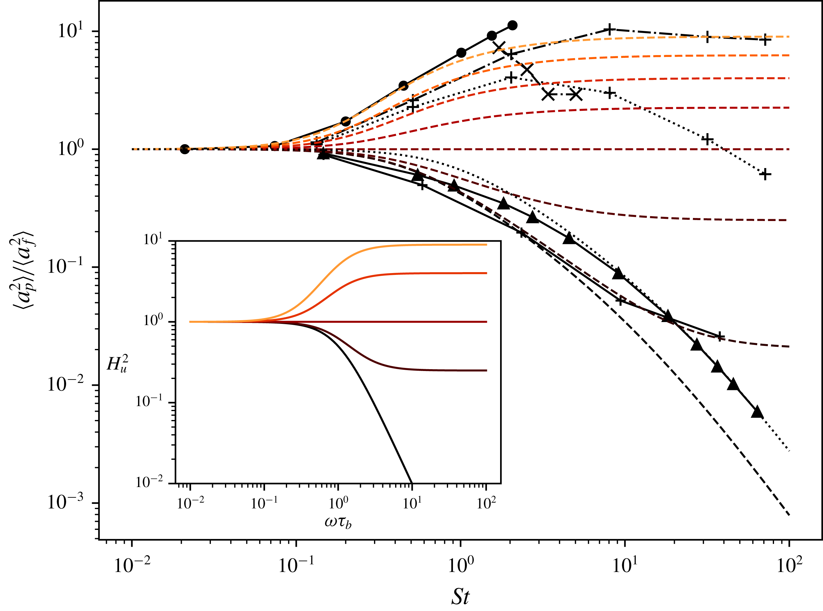
Response of small bubbles and particles to turbulence is known to depend on both Stokes number and $\unicode[STIX]{x1D6FD}$ . This is illustrated in figure 1 which presents the normalized acceleration variance against the Stokes number for various value of $\unicode[STIX]{x1D6FD}$ . In this figure we report the data obtained from our DNS for micro-bubbles ( $\unicode[STIX]{x1D6FD}=3$ ), the DNS for Calzavarini et al. (Reference Calzavarini, Volk, Bourgoin, Lévêque, Pinton and Toschi2009) for light particles ( $\unicode[STIX]{x1D6FD}=2.5$ ) and heavy particles ( $\unicode[STIX]{x1D6FD}=0.14$ ) and the DNS of Bec et al. (Reference Bec, Biferale, Cencini, Lanotte and Toschi2010) for heavy particles ( $\unicode[STIX]{x1D6FD}=0$ ). For the heavy particles ( $\unicode[STIX]{x1D6FD}<1$ ), it is observed that the acceleration variance decreases when the Stokes number increases. This is in contrast to the case of bubbles and light particles ( $\unicode[STIX]{x1D6FD}>1$ ) in which the bubble normalized acceleration variance increases with $St$ .

Figure 1.

Acceleration variance normalized by the fluid tracer acceleration variance from our DNS for bubbles (● and continuous line), the DNS data of Bec et al. (Reference Bec, Biferale, Cencini, Lanotte and Toschi2010) and Lanotte (Reference Lanotte, Calzavarini, Toschi, Bec, Biferale and Cencini2011) for heavy inertial particles $\unicode[STIX]{x1D6FD}=0$ , $Re_{\unicode[STIX]{x1D706}}=400$ (▴ and continuous line), the DNS from Calzavarini et al. (Reference Calzavarini, Volk, Bourgoin, Lévêque, Pinton and Toschi2009) for $\unicode[STIX]{x1D6FD}=2.5$ and $Re_{\unicode[STIX]{x1D706}}=180$ , with and without the Faxén correction ( $+$ with dotted and dot-dashed lines, respectively), and $\unicode[STIX]{x1D6FD}=0.14$ ( $+$ with continuous line), the experimental measurements from Prakash (Reference Prakash2013) for $Re_{\unicode[STIX]{x1D706}}=145-230$ and $\unicode[STIX]{x1D6FD}\approx 3$ ( $\times$ with dashed lines). Comparison with the relation (3.4),  $\langle \boldsymbol{a}_{b}^{2}\rangle (St,\unicode[STIX]{x1D6FD},Re_{0})/\langle \boldsymbol{a}_{b}^{2}\rangle (0,1,Re_{0})$ with $c_{1}=2.8$ and $Re_{0}^{1/2}=0.08Re_{\unicode[STIX]{x1D706}}=16$ for $\unicode[STIX]{x1D6FD}=0$ , 0.14, 0.5, 1, 1.5, 2, 2.5 and 3 from black to orange, in dashed lines, and with $c_{1}=2.8$ and $Re_{0}^{1/2}=0.08Re_{\unicode[STIX]{x1D706}}=32$ , $\unicode[STIX]{x1D6FD}=0$ in black dotted line. The inset is the response function (3.1) as a function of $\unicode[STIX]{x1D714}\unicode[STIX]{x1D70F}_{b}$ for $\unicode[STIX]{x1D6FD}=0$ , 0.5, 1, 2 and 3 from black to orange, respectively.

Based on the dynamics of the bubble given by (2.1) and following the approach of Tchen (Reference Tchen1947) (see also Hinze Reference Hinze1975), one can derive a response function of the bubble velocity fluctuations to the fluid fluctuations, $H_{u}(\unicode[STIX]{x1D714})$ ,

(3.1a,b ) $$\begin{eqnarray}E_{b}(\unicode[STIX]{x1D714})=H_{u}^{2}(\unicode[STIX]{x1D714})E_{f}(\unicode[STIX]{x1D714});\quad H_{u}^{2}(\unicode[STIX]{x1D714})={\displaystyle \frac{1+\unicode[STIX]{x1D6FD}^{2}\unicode[STIX]{x1D714}^{2}\unicode[STIX]{x1D70F}_{b}^{2}}{1+\unicode[STIX]{x1D714}^{2}\unicode[STIX]{x1D70F}_{b}^{2}}},\end{eqnarray}$$

with $\unicode[STIX]{x1D714}$ the pulsation, and where $E_{b}(\unicode[STIX]{x1D714})=\hat{\boldsymbol{u}}_{b}(\unicode[STIX]{x1D714})\hat{\boldsymbol{u}}_{b}(-\unicode[STIX]{x1D714})$ and $E_{f}(\unicode[STIX]{x1D714})=\hat{\boldsymbol{u}}_{f}(\unicode[STIX]{x1D714})\hat{\boldsymbol{u}}_{f}(-\unicode[STIX]{x1D714})$ are the Lagrangian spectra of the bubble and fluid velocity and circumflexes are used to denote the Fourier coefficients. To obtain this relation we assume that the trajectory of the bubble does not deviate significantly from the trajectory of a fluid element as we substitute the material derivative of the fluid velocity by its time derivative along the bubble trajectory. This assumption is questionable as soon as the Stokes number of the bubble is not vanishingly small, and will be discussed later. Anyway, it enables us to easily obtain the qualitative behaviour of the bubble dynamics since in that case, it is not explicitly dependent on the fluid velocity gradient. As shown in the inset of figure 1, the response function differs significantly for a bubble ( $\unicode[STIX]{x1D6FD}=3$ ) and a heavy particle ( $\unicode[STIX]{x1D6FD}=0$ ). While for $\unicode[STIX]{x1D6FD}=0$ , the inertia of the particle filters the high frequency fluctuations of the fluid, for a bubble the high frequency fluctuations of the fluid are amplified. From this relation one can also obtain the response function relating the bubble acceleration fluctuations to the fluid velocity fluctuations along the bubble trajectory, $H_{a}(\unicode[STIX]{x1D714})$ ,

(3.2a,b ) $$\begin{eqnarray}E_{a}(\unicode[STIX]{x1D714})=H_{a}^{2}(\unicode[STIX]{x1D714})E_{f}(\unicode[STIX]{x1D714});\quad H_{a}^{2}=\unicode[STIX]{x1D714}^{2}H_{u}^{2}(\unicode[STIX]{x1D714}),\end{eqnarray}$$

with $E_{a}$ the Lagrangian spectrum of the bubble acceleration. The bubble acceleration variance is given by $\langle \boldsymbol{a}_{b}^{2}\rangle =2\int _{0}^{\infty }E_{a}(\unicode[STIX]{x1D714})\,\text{d}\unicode[STIX]{x1D714}$ . To compute the variance, one needs to prescribe the Lagrangian fluid velocity spectrum along the bubble trajectory. For a fluid tracer the Lagrangian spectrum presents a power law for intermediate frequencies, $E_{f}(\unicode[STIX]{x1D714})\sim \langle \unicode[STIX]{x1D700}\rangle \unicode[STIX]{x1D714}^{-2}$ (Tennekes & Lumley Reference Tennekes and Lumley1972; Yeung Reference Yeung2001). To account for finite Reynolds number effects, and to have a finite energy density for $\unicode[STIX]{x1D714}\rightarrow 0$ we consider the form for the Lagrangian spectra (Hinze Reference Hinze1975; Mordant, Metz & Michel Reference Mordant, Metz and Michel2001) as follows:

(3.3) $$\begin{eqnarray}E_{f}(\unicode[STIX]{x1D714})\approx {\displaystyle \frac{k_{0}\langle \unicode[STIX]{x1D700}\rangle }{\unicode[STIX]{x1D714}^{2}+\unicode[STIX]{x1D714}_{0}^{2}}},\end{eqnarray}$$

with $k_{0}$ a constant, and $\unicode[STIX]{x1D714}_{0}^{-1}$ the Lagrangian integral time scale. Note that the relation (3.3) gives, for the velocity Lagrangian autocorrelation, $\unicode[STIX]{x1D70C}(\unicode[STIX]{x1D70F})=\exp (-\unicode[STIX]{x1D714}_{0}\unicode[STIX]{x1D70F})$ . As shown by Sawford & Yeung (Reference Sawford and Yeung2011), one has $(\unicode[STIX]{x1D70F}_{\unicode[STIX]{x1D702}}\unicode[STIX]{x1D714}_{0})^{-1}=(\unicode[STIX]{x1D714}_{\unicode[STIX]{x1D702}}/\unicode[STIX]{x1D714}_{0})/2\unicode[STIX]{x03C0}\approx 0.08Re_{\unicode[STIX]{x1D706}}$ , with $\unicode[STIX]{x1D714}_{\unicode[STIX]{x1D702}}=2\unicode[STIX]{x03C0}/\unicode[STIX]{x1D70F}_{\unicode[STIX]{x1D702}}$ . For convenience we note in the following $Re_{0}^{1/2}=(\unicode[STIX]{x1D70F}_{\unicode[STIX]{x1D702}}\unicode[STIX]{x1D714}_{0})^{-1}$ . Furthermore the normalizing condition of the spectra, $\langle \boldsymbol{u}_{f}^{2}\rangle =2\int _{0}^{\infty }E_{f}(\unicode[STIX]{x1D714})\,\text{d}\unicode[STIX]{x1D714}$ , gives after integration $\langle \boldsymbol{u}_{f}^{2}\rangle =\unicode[STIX]{x03C0}k_{0}\langle \unicode[STIX]{x1D700}\rangle /\unicode[STIX]{x1D714}_{0}$ that imposes $k_{0}=2(\unicode[STIX]{x1D70F}_{L}/\unicode[STIX]{x1D70F}_{\unicode[STIX]{x1D702}})(\unicode[STIX]{x1D714}_{0}/\unicode[STIX]{x1D714}_{\unicode[STIX]{x1D702}})\approx 4(\unicode[STIX]{x1D70F}_{L}/\unicode[STIX]{x1D70F}_{\unicode[STIX]{x1D702}})Re_{\unicode[STIX]{x1D706}}^{-1}$ with $\unicode[STIX]{x1D70F}_{L}=\langle \boldsymbol{u}_{f}^{2}\rangle /\langle \unicode[STIX]{x1D700}\rangle$ the large eddy time scale. 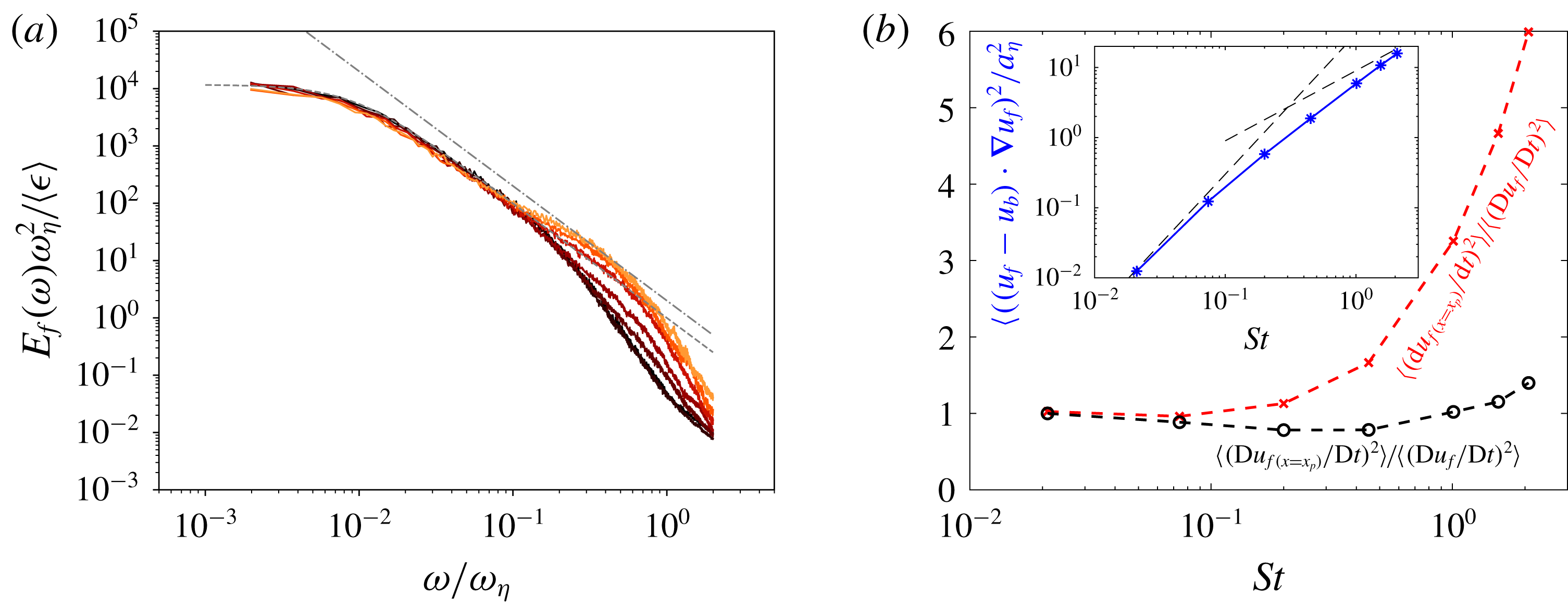This constant is computed from the DNS to be $k_{0}\approx 1.04$ (see table 1). As seen from figure 2(a), with $k_{0}=1.03$ and $\unicode[STIX]{x1D714}_{0}/\unicode[STIX]{x1D714}_{\unicode[STIX]{x1D702}}=0.0092$ , the relation (3.3) provides a very good estimation of $E_{f}$ for the various Stokes number considered here, for $\unicode[STIX]{x1D714}\ll \unicode[STIX]{x1D714}_{\unicode[STIX]{x1D702}}$ . Nevertheless, the high frequency part of the spectra, which presents dependence on the Stokes number, is not predicted correctly by (3.3), an increase in inertia leads to more energy at high frequency. Let us note that for $\unicode[STIX]{x1D6FD}>0$ the previous integral only converges if $E_{f}(\unicode[STIX]{x1D714})$ decreases fast enough at large $\unicode[STIX]{x1D714}$ . Therefore to ensure its convergence, the integral is truncated above $k_{1}\unicode[STIX]{x1D714}_{\unicode[STIX]{x1D702}}$ , independently of the Stokes number. This gives for the bubble acceleration variance the following relation:

(3.4) $$\begin{eqnarray}\langle \boldsymbol{a}_{b}^{2}\rangle \approx c_{0}a_{\unicode[STIX]{x1D702}}^{2}\left[\unicode[STIX]{x1D6FD}^{2}+{\displaystyle \frac{1-\unicode[STIX]{x1D6FD}^{2}}{1-St_{0}^{2}}}{\displaystyle \frac{\tan ^{-1}(c_{1}St)}{c_{1}St}}-{\displaystyle \frac{1-\unicode[STIX]{x1D6FD}^{2}St_{0}^{2}}{1-St_{0}^{2}}}{\displaystyle \frac{\tan ^{-1}(c_{1}Re_{0}^{1/2})}{c_{1}Re_{0}^{1/2}}}\right],\end{eqnarray}$$

with $c_{1}=2\unicode[STIX]{x03C0}k_{1}$ , $c_{0}=4\unicode[STIX]{x03C0}k_{1}k_{0}$ and $St_{0}=St/Re_{0}^{1/2}$ a Stokes number based on the large eddy time scale. Note that the previous relation does not present singularities for $St_{0}=1$ since in this case the last two terms cancel. Also $\langle \boldsymbol{a}_{b}^{2}\rangle$ remains positive for all $St$ , $Re_{0}$ and $\unicode[STIX]{x1D6FD}$ . Nevertheless, the assumptions used to derive (3.4) are a priori satisfied for $Re_{0}\gg St^{2}$ and $Re_{0}\gg 1$ , and in this limit (3.4) becomes

(3.5) $$\begin{eqnarray}\langle \boldsymbol{a}_{b}^{2}\rangle \approx c_{0}a_{\unicode[STIX]{x1D702}}^{2}\left[\unicode[STIX]{x1D6FD}^{2}+(1-\unicode[STIX]{x1D6FD}^{2}){\displaystyle \frac{\tan ^{-1}(c_{1}St)}{c_{1}St}}\right].\end{eqnarray}$$

A similar relation is proposed by Zaichik & Alipchenkov (Reference Zaichik and Alipchenkov2011). Their derivation is based on the same approximation for the fluid acceleration and assumes the fluid velocity correlation in physical space that include a viscous cutoff at small scale contrary to the relation (3.3) used here. The relation (3.4) with $c_{1}=2.8$ and $Re_{0}^{1/2}=16$ is plotted in figure 1 for various $St$ and $\unicode[STIX]{x1D6FD}$ . In this figure, the bubble acceleration variance is normalized by the acceleration variance of fluid tracers estimated from the model (3.4) by setting $St=0$ and $\unicode[STIX]{x1D6FD}=1$ . It is seen that (3.4) is overall in good agreement with the DNS data sets for $\unicode[STIX]{x1D6FD}=3$ , 2.5, 0.14 and 0. The discrepancy between the DNS and relation (3.4) observed for the inertial particles around $St=1$ , is attributed to the preferential concentration of particles, since this effect is not accounted for in the model. For the inertial particles at $St\approx 0.5$ the model overestimates the acceleration by approximately 20 %. It is also observed that for $St>1$ , (3.4) underestimates the DNS when $\unicode[STIX]{x1D6FD}=3$ and $2.5$ . Note also that the evolution of the acceleration variance with $St$ and $\unicode[STIX]{x1D6FD}$ given by the model (3.4) appears qualitatively similar to the DNS data presented by Volk et al. (Reference Volk, Calzavarini, Verhille, Lohse, Mordant, Pinton and Toschi2008a ). As expected, the acceleration variance normalized by the acceleration variance of fluid tracer tends to unity when $St$ goes to 0 for every value of $\unicode[STIX]{x1D6FD}$ , indicating that bubbles with bubbles with extremely small diameter effectively behave as fluid tracers. According to (3.4) for $\unicode[STIX]{x1D6FD}=0$ , the decrease of the acceleration variance with the Stokes number presents the same scaling as the relation proposed by Gorokhovski & Zamansky (Reference Gorokhovski and Zamansky2018), namely $\langle \boldsymbol{a}_{b}^{2}\rangle /a_{\unicode[STIX]{x1D702}}^{2}\approx 1$ for $St\ll 1$ , $\langle \boldsymbol{a}_{b}^{2}\rangle /a_{\unicode[STIX]{x1D702}}^{2}\sim St^{-1}$ for $1\ll St\ll \sqrt{Re_{0}}$ and $\langle \boldsymbol{a}_{b}^{2}\rangle /a_{\unicode[STIX]{x1D702}}^{2}\sim St^{-2}$ for $St\gg \sqrt{Re_{0}}$ and appears consistent with the relation proposed by Bec et al. (Reference Bec, Biferale, Boffetta, Celani, Cencini, Lanotte, Musacchio and Toschi2006).

Figure 2.

(a) Lagrangian fluid velocity spectra along the bubble trajectory from the DNS for $St=0.02$ , 0.074, 0.20, 0.45, 1.01, 1.55 and 2.07 (from black to red, respectively). Comparison with the power law $\unicode[STIX]{x1D714}^{-2}$ and the relation (3.3),  $k_{0}/((\unicode[STIX]{x1D714}/\unicode[STIX]{x1D714}_{\unicode[STIX]{x1D702}})^{2}+(\unicode[STIX]{x1D714}_{0}/\unicode[STIX]{x1D714}_{\unicode[STIX]{x1D702}})^{2})$ with $k_{0}=1$ and $\unicode[STIX]{x1D714}_{0}/\unicode[STIX]{x1D714}_{\unicode[STIX]{x1D702}}=0.0092$ in grey dot-dashed and dashed lines, respectively. (b) Evolution with the Stokes number of the variance of the material derivative of fluid velocity at the bubble position (black circles) and of the Lagrangian time derivative along the bubble trajectories of the fluid velocity (red crosses). Both quantities are normalized by the global variance of the fluid tracer acceleration. The inset is the variance of the difference between these two quantities in logarithmic scales normalized by the Kolmogorov acceleration and comparison with the $St$ and $St^{1/2}$ power laws.

In contrast, for a bubble ( $\unicode[STIX]{x1D6FD}=3$ ), according to (3.4), the normalized acceleration variance increases as $\langle \boldsymbol{a}_{b}^{2}\rangle /a_{\unicode[STIX]{x1D702}}^{2}-1\sim St^{2}$ and saturates to $\unicode[STIX]{x1D6FD}^{2}$ for $St\gg 1$ . Note, however, that the limit $St\gg 1$ does not make sense, since for a bubble it implies $d_{b}^{2}/\unicode[STIX]{x1D702}^{2}\gg 1$ which disagrees with the pointwise model. From the experimental results of Prakash et al. (Reference Prakash, Tagawa, Calzavarini, Mercado, Toschi, Lohse and Sun2012) and the numerical simulations with a Faxén correction term (Calzavarini et al. Reference Calzavarini, Volk, Bourgoin, Lévêque, Pinton and Toschi2009), also plotted in figure 1 for completeness, it appears that the finite size effect becomes important from $St\approx 2$ or $d_{b}/\unicode[STIX]{x1D702}\approx 7$ , and leads to a decrease of the acceleration variance with a further increase of the bubble diameter (or Stokes number).

To analyse the substitution of the fluid velocity material derivative at the bubble position, $\text{D}\boldsymbol{u}_{f}/\text{D}t$ , by its Lagrangian derivative along the bubble trajectory, $\text{d}\boldsymbol{u}_{f}/\text{d}t$ , implied in (3.1), we remark that the material derivative can be written as $\text{D}\boldsymbol{u}_{f}/\text{D}t=\text{d}\boldsymbol{u}_{f}/\text{d}t+(\boldsymbol{u}_{f}-\boldsymbol{u}_{p})\boldsymbol{\cdot }\unicode[STIX]{x1D735}\boldsymbol{u}_{f}$ . We estimate that the order of magnitude of the last term is $O((\boldsymbol{u}_{f}-\boldsymbol{u}_{p})\boldsymbol{\cdot }\unicode[STIX]{x1D735}\boldsymbol{u}_{f})=\langle \boldsymbol{F}_{d}^{2}\rangle ^{1/2}St$ , $\boldsymbol{F}_{d}$ being the drag force. Therefore, based on the previously disused scaling of the inertial particle acceleration we expect that this term grows linearly with $St$ for $St\ll 1$ and as $St^{1/2}$ for $1\ll St\ll \sqrt{Re_{0}}$ (see also the relation for the variance of the drag force proposed latter in (3.6)). Note that to obtain the previous estimation we have assumed that velocity gradients are of order $1/\unicode[STIX]{x1D70F}_{\unicode[STIX]{x1D702}}$ and thus we neglected intermittency effects which probably leads to an underestimation at large Reynolds numbers. As shown in the inset of figure 2(b) the proposed scaling for the difference appears to be consistent with the DNS. To analyse further the error due to the simplification of the fluid inertia term we have computed, from the DNS, the variances of $\text{D}\boldsymbol{u}_{f}/\text{D}t$ and $\text{d}\boldsymbol{u}_{f}/\text{d}t$ . It is seen in figure 2(b) that for $St<0.2$ the variance of the time derivative of the fluid velocity along the bubble trajectory remains sizable to the variance of the fluid acceleration at the bubble position (around 10 % of difference) while, for $St=1$ , it is larger by a factor of roughly 3. Moreover, the normalized p.d.f. of these two quantities (not shown) remains quite similar even for the largest Stokes number considered here. We can then conclude that our approximation is reasonable for $St<1$ and could lead to an overestimation of the fluid inertia term for larger $St$ . Nevertheless, the range of validity of the substitution and of the pointwise bubble approximation are seen to coincide.

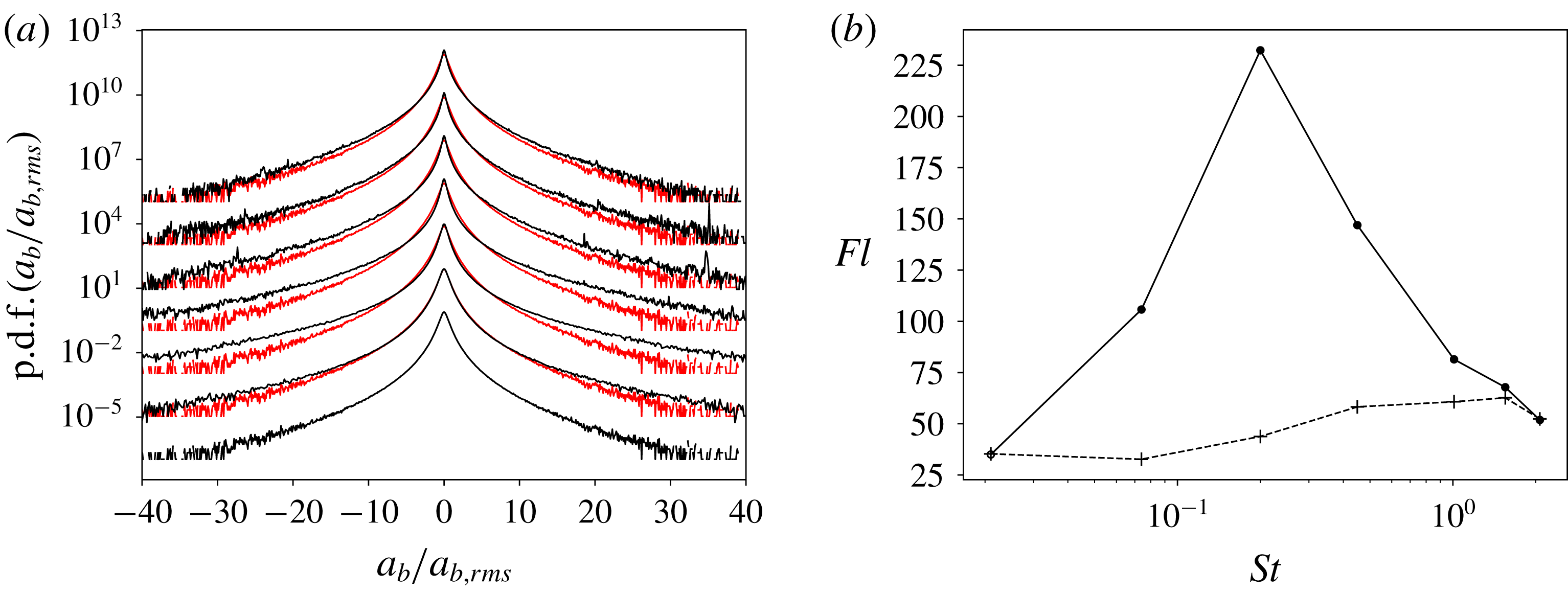
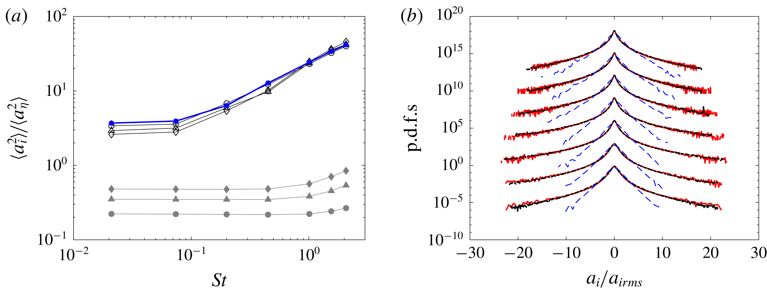
The expression (3.5) does not include any intermittency effects and Reynolds number dependence (Yeung et al. Reference Yeung, Pope, Lamorgese and Donzis2006). The intermittent behaviour of the dissipation rate which is accounted for by the stochastic models discussed in § 4 is associated with large fluctuations of the acceleration (Kolmogorov Reference Kolmogorov1962; Castaing, Gagne & Hopfinger Reference Castaing, Gagne and Hopfinger1990; Lukassen & Wilczek Reference Lukassen, Wilczek, Örlü, Talamelli, Oberlack and Peinke2017). This is seen in figure 3 presenting the bubble acceleration p.d.f. obtained from the DNS. It is observed that the bubble acceleration p.d.f. clearly presents a non-Gaussian behaviour with stretched tails indicating the occurrence of very intense acceleration events as pointed by Volk et al. (Reference Volk, Calzavarini, Verhille, Lohse, Mordant, Pinton and Toschi2008a ), Prakash et al. (Reference Prakash, Tagawa, Calzavarini, Mercado, Toschi, Lohse and Sun2012) and Loisy & Naso (Reference Loisy and Naso2017). For intermediate Stokes number ( $St\approx 0.5$ ) the bubble acceleration p.d.f. appears even more stretched than the p.d.f. of fluid tracer acceleration. While a further increase of $St$ gives again a p.d.f. very similar to the p.d.f. of fluid tracer acceleration. Correspondingly, figure 3(b) shows that the bubble acceleration flatness ( $Fl_{a}=\langle (\boldsymbol{a}_{b}-\langle \boldsymbol{a}_{b}\rangle )^{4}\rangle /\langle (\boldsymbol{a}_{b}-\langle \boldsymbol{a}_{b}\rangle )^{2}\rangle ^{2}$ ) presents a maximum for a Stokes number around $0.2$ . Note that a peak was also observed in Calzavarini et al. (Reference Calzavarini, Volk, Bourgoin, Lévêque, Pinton and Toschi2009) but with a smaller maximum value and for a larger value of $St$ . The difference is attributed to the smaller value of $\unicode[STIX]{x1D6FD}$ and $Re_{\unicode[STIX]{x1D706}}$ ( $\unicode[STIX]{x1D6FD}=2.5$ and $Re_{\unicode[STIX]{x1D706}}=75$ ) used in Calzavarini et al. (Reference Calzavarini, Volk, Bourgoin, Lévêque, Pinton and Toschi2009). In this figure we also compare the flatness of fluid acceleration at the bubble position (or equivalently the flatness of the inertia force). It is observed that its value increases with $St$ , but remains much smaller than the bubble acceleration flatness for intermediate Stokes numbers. As discussed below, the non-monotonic evolution of the bubble acceleration flatness is attributed to specific geometrical arrangements of the hydrodynamic forces applied to the bubble, rather than to a preferential concentration of bubbles in special regions of the flow (Calzavarini et al. Reference Calzavarini, Kerscher, Lohse and Toschi2008; Tagawa et al. Reference Tagawa, Mercado, Prakash, Calzavarini, Sun and Lohse2012). Given the very large values taken by the flatness, this statistic might not be well converged, nevertheless there is no doubt that the flatness of the acceleration of the bubbles is much greater than that of the acceleration of the fluid at the bubble position.

Figure 3.

(a) The p.d.f.s of the bubble acceleration normalized by its root-mean-square value in black for $St=0.02$ , 0.074, 0.20, 0.45, 1.01, 1.55 and 2.07 (shifted upward by two decades from each other for clarity, respectively) and comparison with the p.d.f.s of the acceleration of fluid tracers in red. (b) Flatness of the bubble acceleration (●) and of the fluid acceleration at the bubble position ( $+$ ) against $St$ from our DNS.

From the relation (3.1) it is as well possible to obtain an estimate for the variance of the two terms on the right-hand side of (2.1), the drag force $\boldsymbol{F}_{D}=-(1/\unicode[STIX]{x1D70F}_{b})(\boldsymbol{u}_{b}(t)-\boldsymbol{u}_{f}(\boldsymbol{x}=\boldsymbol{x}_{b}(t),t))$ , and the fluid inertia effect $\boldsymbol{F}_{I}=\unicode[STIX]{x1D6FD}(\text{D}\boldsymbol{u}_{f}/\text{D}t)(\boldsymbol{x}=\boldsymbol{x}_{b}(t),t)$ ,

(3.6) $$\begin{eqnarray}\displaystyle \langle \boldsymbol{F}_{D}^{2}\rangle & {\approx} & \displaystyle \int _{0}^{k_{1}\unicode[STIX]{x1D714}_{\unicode[STIX]{x1D702}}}E_{f}(\unicode[STIX]{x1D714}){\displaystyle \frac{\unicode[STIX]{x1D714}^{2}(1-\unicode[STIX]{x1D6FD})^{2}}{1+\unicode[STIX]{x1D714}^{2}\unicode[STIX]{x1D70F}_{b}^{2}}}\,\text{d}\unicode[STIX]{x1D714}\nonumber\\ \displaystyle & {\approx} & \displaystyle c_{0}a_{\unicode[STIX]{x1D702}}^{2}{\displaystyle \frac{(1-\unicode[STIX]{x1D6FD})^{2}}{1-St_{0}^{2}}}\left({\displaystyle \frac{\tan ^{-1}(c_{1}St)}{c_{1}St}}-{\displaystyle \frac{\tan ^{-1}(c_{1}Re_{0}^{1/2})}{c_{1}Re_{0}^{1/2}}}\right)\end{eqnarray}$$

(3.7) $$\begin{eqnarray}\displaystyle \langle \boldsymbol{F}_{I}^{2}\rangle & {\approx} & \displaystyle \int _{0}^{k_{1}\unicode[STIX]{x1D714}_{\unicode[STIX]{x1D702}}}E_{f}(\unicode[STIX]{x1D714})\unicode[STIX]{x1D714}^{2}\unicode[STIX]{x1D6FD}^{2}\,\text{d}\unicode[STIX]{x1D714}\nonumber\\ \displaystyle & {\approx} & \displaystyle c_{0}a_{\unicode[STIX]{x1D702}}^{2}\unicode[STIX]{x1D6FD}^{2}\left(1-{\displaystyle \frac{\tan ^{-1}(c_{1}Re_{0}^{1/2})}{c_{1}Re_{0}^{1/2}}}\right).\end{eqnarray}$$

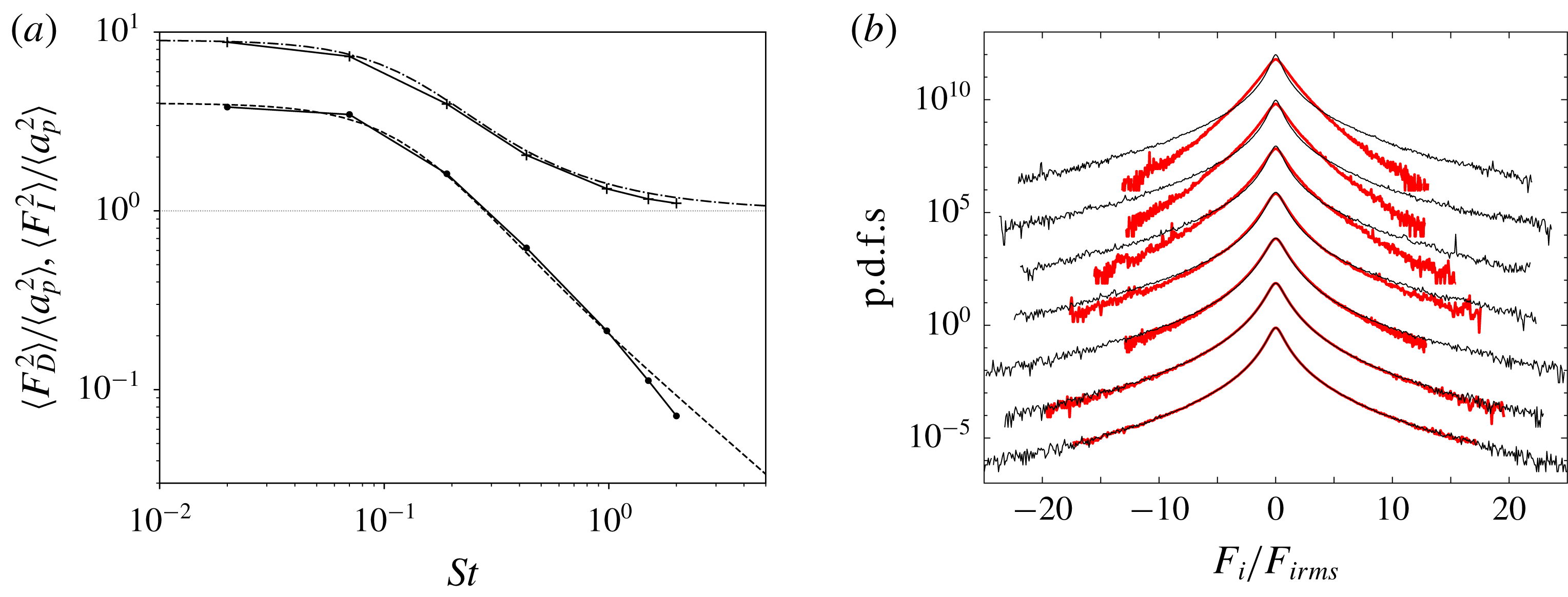
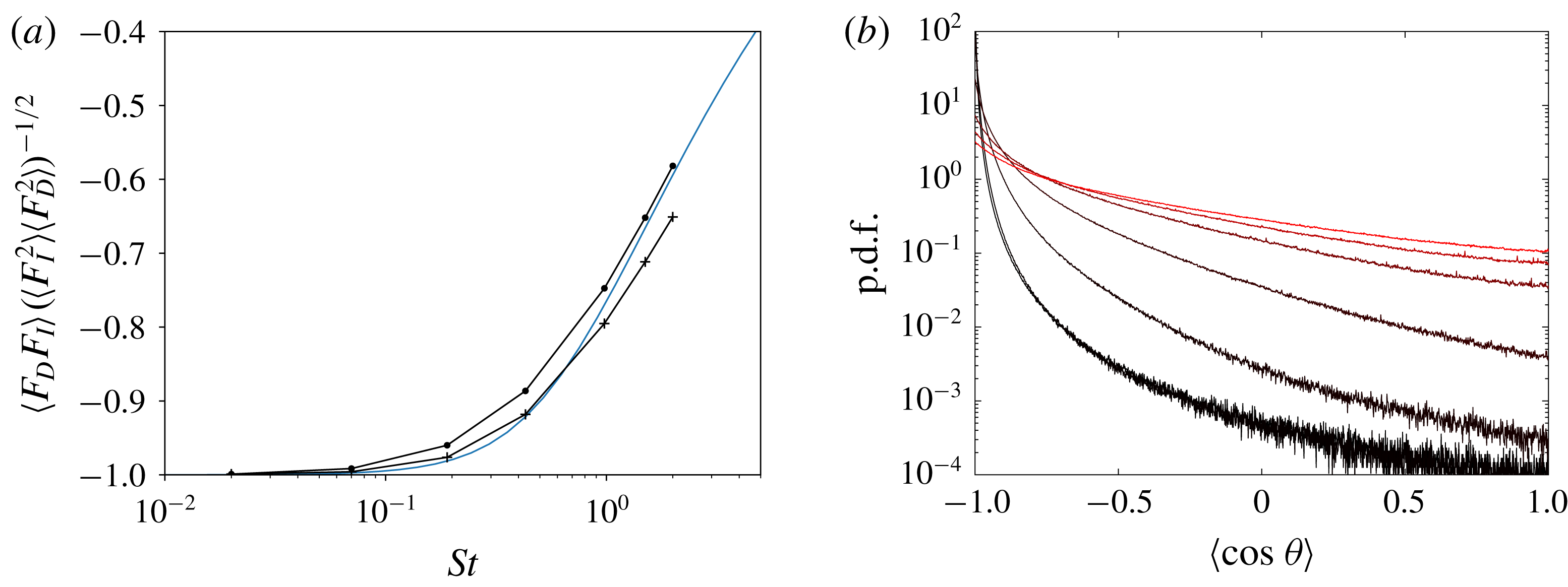
These relations are plotted in figure 4(a) and are compared with the variance of the forces obtained from our DNS. Similar to the estimation of the acceleration variance expressions (3.6) and (3.7) are seen to provide a good estimation of the variances of $\boldsymbol{F}_{D}$ and $\boldsymbol{F}_{I}$ although the drag force is overestimated and the inertia force given by (3.7) is independent of the Stokes number which disagrees with the observation of figure 2(b). It is seen that for small Stokes numbers the variance of the two forces are commensurate, although the fluid inertia effect is dominant. Precisely, for $St\rightarrow 0$ the variance of the drag force is $(2/3)^{2}$ of that of the inertia term. It is also observed that the sum of the variance of the two forces is much larger than the variance of the bubble acceleration indicating a significant correlation between the two terms. As expected, when the Stokes number is increased, the drag force becomes negligible and the bubble acceleration is essentially given by the fluid inertia term.

Figure 4(b) presents the p.d.f. of both drag and fluid inertia forces for the various Stokes numbers. It is observed that for vanishingly small Stokes numbers ( $St=0.02$ ) the p.d.f.s of the two forces are essentially identical, and present both developed tails. The increase of the Stokes number results in a significant reduction of the tails of the drag force’s p.d.f. whereas the p.d.f. of the inertia force presents very little variation (see also its flatness in figure 3). It is also worth mentioning that the p.d.f. of both forces remain symmetrical for all Stokes number indicating that the average and the skewness values of the two forces are zero. Because the bubbles sample regions of the flow in which the fluid acceleration variance is slightly below its overall value (see figure 2) and that the p.d.f. of the fluid acceleration at the bubble position is nearly invariant with the Stokes number, we conclude that the maximum of the bubble acceleration flatness is not caused by preferential concentration effects but is rather due to the alignment of the hydrodynamic forces on the bubble.

Figure 4.

(a) Evolution with the Stokes number of the variance of the drag force (circle) and inertia force (crosses) relative to the bubble acceleration variance according to our DNS and comparison with (3.6) and (3.7) normalized by (3.4) with $c_{1}=2.8$ and $Re_{0}^{1/2}=16$ in dashed and dot-dashed lines, respectively. (b) The p.d.f. of the fluid inertia forces (black) and of the drag force (red) normalized by their root-mean-square value for $St=0.02$ , 0.074, 0.20, 0.45, 1.01, 1.55 and 2.07 (shifted upward by one decade from each other for clarity, respectively).

In figure 5(a), we plot the evolution of the correlation between $\boldsymbol{F}_{D}$ and $\boldsymbol{F}_{I}$ with the Stokes number obtained from the DNS. It is seen that for small $St$ the two forces are completely anticorrelated, while they progressively decorrelate as $St$ increases. Indeed requiring that for $St=0$ the acceleration is equal to the acceleration of a fluid tracer, we obtain from (2.1) that $\boldsymbol{F}_{D}=(1-\unicode[STIX]{x1D6FD})/\unicode[STIX]{x1D6FD}\boldsymbol{F}_{I}$ , that gives an anti-alignment for $\unicode[STIX]{x1D6FD}>1$ . Further, the correlation can also be readily estimated for larger Stokes numbers from (3.6), (3.7) and (3.4) as follows:

(3.8) $$\begin{eqnarray}\langle \boldsymbol{F}_{D}\boldsymbol{\cdot }\boldsymbol{F}_{I}\rangle \approx c_{0}a_{\unicode[STIX]{x1D702}}^{2}{\displaystyle \frac{\unicode[STIX]{x1D6FD}(1-\unicode[STIX]{x1D6FD})}{1-St_{0}^{2}}}\left({\displaystyle \frac{\tan ^{-1}(c_{1}St)}{c_{1}St}}-{\displaystyle \frac{\tan ^{-1}(c_{1}Re_{0}^{1/2})}{c_{1}Re_{0}^{1/2}}}\right).\end{eqnarray}$$

Figure 5(a) shows that the relation (3.8) is in good agreement with the DNS results. Further, if the persistence of the temporal autocorrelation of the norms of the two forces is much longer than for their orientation, then the correlation between the two forces could be approximated by their relative orientation,

(3.9) $$\begin{eqnarray}\langle \boldsymbol{F}_{D}\boldsymbol{\cdot }\boldsymbol{F}_{I}\rangle \approx \langle \cos \unicode[STIX]{x1D703}\rangle (\langle \boldsymbol{F}_{D}^{2}\rangle \langle \boldsymbol{F}_{I}^{2}\rangle )^{1/2},\end{eqnarray}$$

where $\unicode[STIX]{x1D703}$ is defined as $\cos \unicode[STIX]{x1D703}=\boldsymbol{F}_{D}\boldsymbol{\cdot }\boldsymbol{F}_{I}/|\boldsymbol{F}_{D}||\boldsymbol{F}_{I}|=\boldsymbol{e}_{I}\boldsymbol{\cdot }\boldsymbol{e}_{D}$ , with $\boldsymbol{e}_{I}$ and $\boldsymbol{e}_{D}$ the orientation vectors of the inertia term and of the drag force, respectively. This is confirmed in figure 5(a) that indeed $\langle \cos \unicode[STIX]{x1D703}\rangle$ remains quite close to $\langle \boldsymbol{F}_{D}\boldsymbol{\cdot }\boldsymbol{F}_{I}\rangle (\langle \boldsymbol{F}_{D}^{2}\rangle \langle \boldsymbol{F}_{I}^{2}\rangle )^{-1/2}$ . Figure 5(b) reports the evolution with the Stokes number of the p.d.f. of $\cos \unicode[STIX]{x1D703}$ . For small Stokes numbers, the two forces appear to be essentially anti-aligned as the p.d.f. presents a sharp peak around $-1$ consistent with its averaged value. When the Stokes number is increased, the distribution of $\cos \unicode[STIX]{x1D703}$ becomes flatter, indicating that the relative orientation of the two forces becomes progressively statistically isotropic. Note that according to (3.8) we should expect a positive correlation between the two forces for $\unicode[STIX]{x1D6FD}<1$ and small $St$ .

Figure 5.

(a) Evolution with $St$ of the coefficient of correlation between the drag and inertia forces (dots) and of $\langle \cos \unicode[STIX]{x1D703}\rangle$ ( $\unicode[STIX]{x1D703}$ being the relative orientation of the forces) (crosses) from the DNS and comparison with relation (3.8) normalized by (3.6) and (3.7) with $c_{1}=2.8$ and $Re_{0}^{1/2}=16$ in blue lines. (b) The p.d.f.s of the cosine of the angle $\unicode[STIX]{x1D703}$ between the two forces, for $St=0.02$ , 0.074, 0.20, 0.45, 1.01, 1.55 and 2.07 (from black to red, respectively).

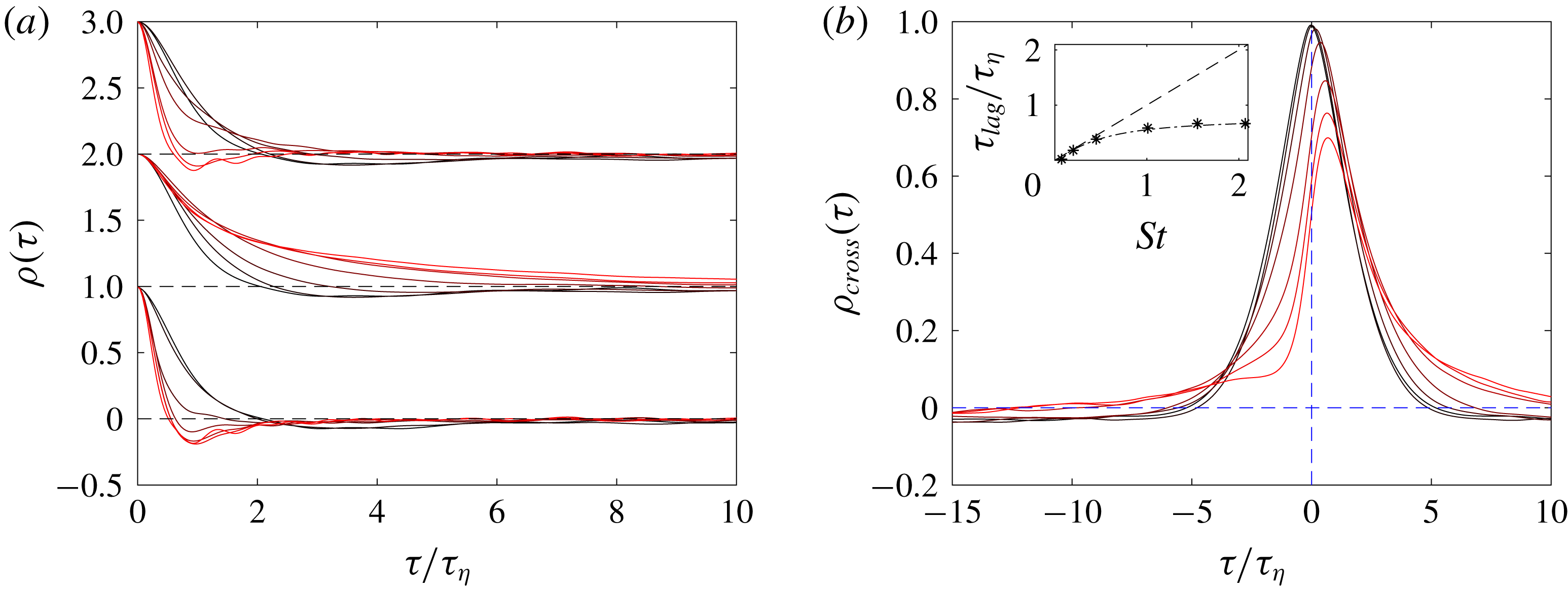
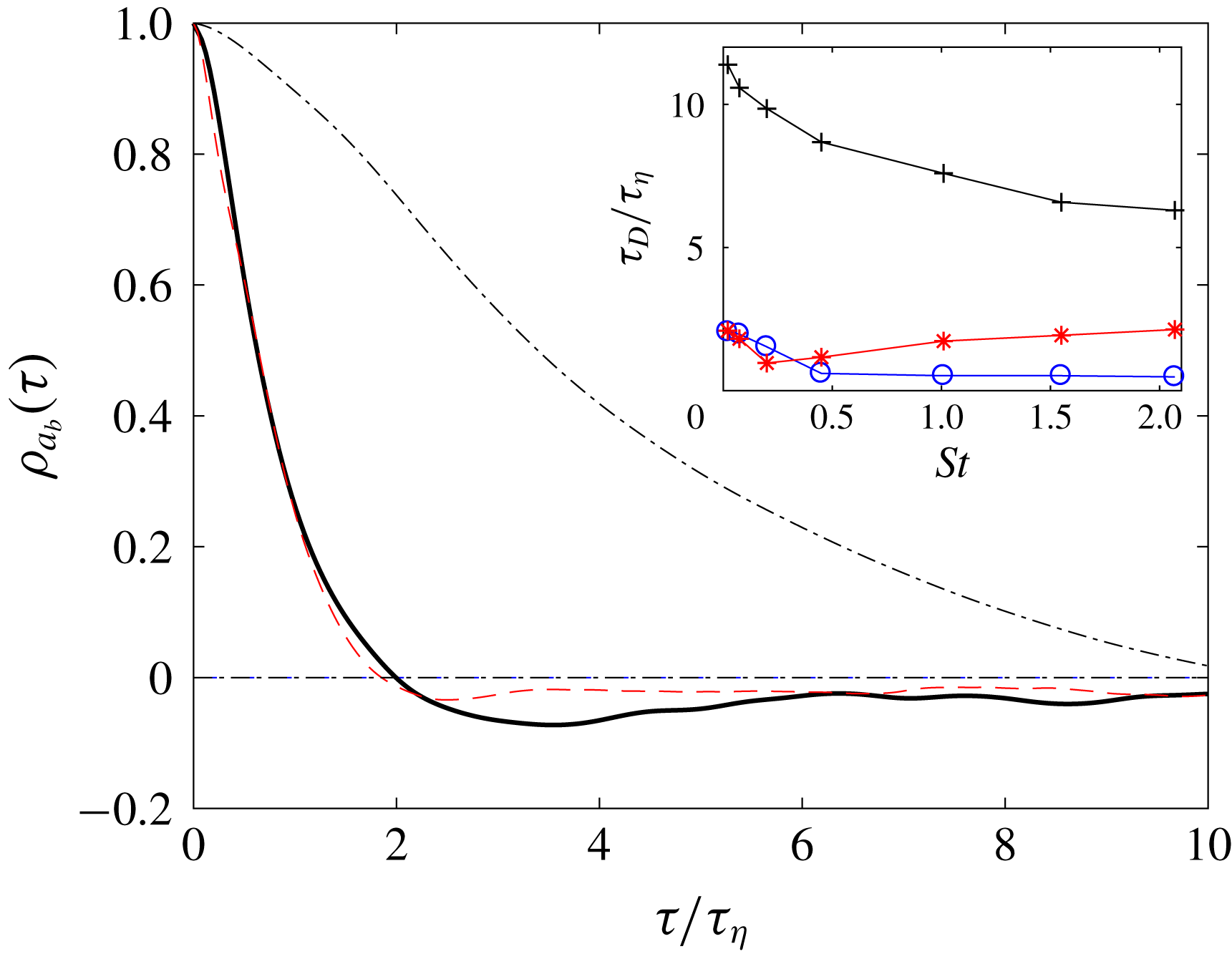
In figure 6(a), we present the evolution of the Lagrangian autocorrelation of the bubble acceleration for the various Stokes numbers. It is observed that an increase of the Stokes number produces a faster decorrelation, as already reported by Volk et al. (Reference Volk, Mordant, Verhille and Pinton2008b ), although for $0<St<2$ it is seen that the correlation time remains of order $\unicode[STIX]{x1D70F}_{\unicode[STIX]{x1D702}}$ . It is worth mentioning that this behaviour departs significantly from the evolution of inertial particles which present larger correlation time with increasing $St$ (Gorokhovski & Zamansky Reference Gorokhovski and Zamansky2018). To further analyse this point, we also present, in figure 6(a), the autocorrelation along the bubble trajectory of the two forces acting on the bubble. It is observed that for vanishingly small Stokes number, the two forces present exactly the same evolution of their Lagrangian correlation, because of the almost instantaneous response of the drag force to the inertia force. With increasing the Stokes number, one sees a clear difference in the autocorrelation of the drag force and of the inertia forces. Increasing the Stokes number gives a longer persistence time for the drag forces which can be directly attributed to the increase of $\unicode[STIX]{x1D70F}_{b}$ . On the other hand, the faster decorrelation of the inertia force is explained by the deviation of the bubble trajectories from the fluid tracer trajectories.

The response of the drag force to the inertia term is analysed in figure 6(b) which presents the plot of the cross correlation of the orientation of the two forces along the bubble trajectory. The cross-correlation is defined as $\unicode[STIX]{x1D70C}_{e_{D},e_{I}}=\langle -\boldsymbol{e}_{I}(t)\boldsymbol{\cdot }\boldsymbol{e}_{D}(t+\unicode[STIX]{x1D70F})\rangle /(\langle \boldsymbol{e}_{I}^{2}\rangle \langle \boldsymbol{e}_{D}^{2}\rangle )^{1/2}$ . This figure confirms that the orientation of the drag forces responds to the inertia term. The temporal lag between the two forces can be estimated from the time shift of the peak, $\max _{\unicode[STIX]{x1D70F}}(\unicode[STIX]{x1D70C}_{e_{D},e_{I}}(\unicode[STIX]{x1D70F}))=\unicode[STIX]{x1D70C}_{e_{D},e_{I}}(\unicode[STIX]{x1D70F}_{lag})$ . In the inset of figure 6(a), we present the evolution of $\unicode[STIX]{x1D70F}_{lag}$ with $St$ . It is seen that $\unicode[STIX]{x1D70F}_{lag}$ presents a linear evolution for small $\unicode[STIX]{x1D70F}_{b}$ . Indeed for vanishingly small Stokes number, the drag responds instantaneously. For larger Stokes number, the growth rate of $\unicode[STIX]{x1D70F}_{lag}$ reduces. We observe that $\unicode[STIX]{x1D70F}_{lag}\approx \unicode[STIX]{x1D70F}_{\unicode[STIX]{x1D702}}(\unicode[STIX]{x1D6FD}-1)^{-1}\tan ^{-1}((\unicode[STIX]{x1D6FD}-1)St)$ is a relatively good approximation of the lag of the drag force compared to the inertia effect. Clearly a further check of this speculative relation would require simulations for different values of $\unicode[STIX]{x1D6FD}$ . We remark that one could estimate the autocorrelation of the bubble acceleration or hydrodynamic forces as well as the cross-correlation presented in figure 6 from the spectral response model of (3.1). However, this would require a more precise estimation of the Lagrangian fluid velocity spectra at high frequency than the relation (3.3), as the decorrelation is controlled by the dissipative range of the spectra which depend on $St$ as seen in figure 2.

Figure 6.

(a) Autocorrelation coefficient of the bubble acceleration, drag force and fluid inertia terms (shifted upward by one unit from each other, respectively, for clarity) from our DNS. (b) Cross-correlation between the drag force and the fluid inertia term as given by our DNS. The inset is the evolution of the time lag (defined as the time of the peak of cross-correlation) with $St$ , and comparison with the $\unicode[STIX]{x1D70F}_{lag}/\unicode[STIX]{x1D70F}_{\unicode[STIX]{x1D702}}=St$ and $\unicode[STIX]{x1D70F}_{lag}/\unicode[STIX]{x1D70F}_{\unicode[STIX]{x1D702}}=(\unicode[STIX]{x1D6FD}-1)^{-1}\tan ^{-1}((\unicode[STIX]{x1D6FD}-1)St)$ . For both figures $St=0.02$ , 0.074, 0.20, 0.45, 1.01, 1.55 and 2.07 (from black to red, respectively).

The anti-alignment of the forces at small Stokes can be explained as follows. For vanishingly small Stokes number, the relaxation time $\unicode[STIX]{x1D70F}_{b}$ of the bubble velocity to the local fluid velocity is much smaller than the persistence time of the fluid inertia term, which is of order $\unicode[STIX]{x1D70F}_{\unicode[STIX]{x1D702}}$ (Pope Reference Pope1990; Mordant et al. Reference Mordant, Crawford and Bodenschatz2004). Therefore, the drag force will very quickly respond, leading it to be statistically opposed to the fluid inertia term. On the other hand, for $St\gg 1$ we should expect that the orientation of the two forces becomes independent because the relaxation time of the particle becomes much larger than $\unicode[STIX]{x1D70F}_{\unicode[STIX]{x1D702}}$ . In the meantime, we have observed that the amplitude of the drag forces becomes negligible as the Stokes number is increased. This conjunction of the evolution of the relative orientation and magnitude of the two forces, leads to the increases of the bubble acceleration flatness, observed in figure 3 for $St$ around 0.5. For these Stokes numbers, the amplitude of the drag forces remains significant while its orientation already presents a wide distribution, leading to the strong intermittency of the acceleration, when the two forces, of similar magnitude, are anti-aligned the acceleration will be close to zero whereas in case of an alignment of the forces intense acceleration will result.

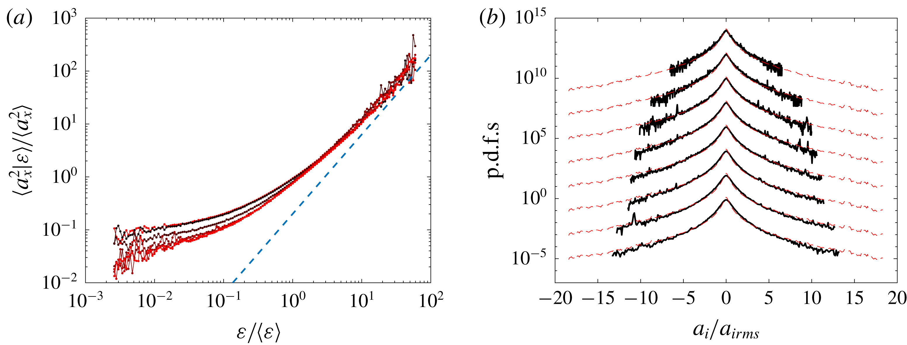
We have proposed above a relation between the bubble acceleration variance and the average dissipation rate. However, in line with the Kolmogorov theory, the instantaneous acceleration depends a priori on the local energy dissipation rate $\unicode[STIX]{x1D700}$ . To discuss this point we present in figure 7 statistics of the bubble acceleration conditioned on the local value of the dissipation rate. This is also motivated to provide supports for a stochastic modelling of the bubble acceleration that accounts for the large fluid fluctuations in small-scale motions, as discuss in the following section. We consider in figure 7(a) the variance of the bubble acceleration conditioned on the local dissipation rate. We first observe that for $\unicode[STIX]{x1D700}$ larger than its average value, $\langle \boldsymbol{a}_{b}^{2}|\unicode[STIX]{x1D700}\rangle$ appears to be independent of the Stokes number, and increases as $\unicode[STIX]{x1D700}^{3/2}$ , while it presents little dependence on both $\unicode[STIX]{x1D700}$ and $St$ for small value of $\unicode[STIX]{x1D700}$ ,

(3.10) $$\begin{eqnarray}\langle \boldsymbol{a}_{b}^{2}|\unicode[STIX]{x1D700}\rangle \approx \langle \boldsymbol{a}_{b}^{2}\rangle \left({\displaystyle \frac{\unicode[STIX]{x1D700}}{\langle \unicode[STIX]{x1D700}\rangle }}\right)^{3/2};\quad \unicode[STIX]{x1D700}>\langle \unicode[STIX]{x1D700}\rangle .\end{eqnarray}$$

This behaviour is similar to previous observations for fluid tracers from Yeung et al. (Reference Yeung, Pope, Lamorgese and Donzis2006). The invariance with $St$ observed for the micro-bubbles is therefore attributed to dominance of the fluid inertia term. It was reported by Yeung et al. (Reference Yeung, Pope, Lamorgese and Donzis2006) that the exponent of the power law for the conditional acceleration is reduced for low values of Reynolds numbers. Also Yeung et al. (Reference Yeung, Pope, Lamorgese and Donzis2006) showed that the value at which the acceleration variance converge for $\unicode[STIX]{x1D700}\rightarrow 0$ decreases with Reynolds number, indicating that the acceleration in the weakly dissipative regions is primarily influenced by the large-scale sweeping. In figure 7(b) the conditional p.d.f. normalized by its standard deviation is shown to be approximately self-similar with $\unicode[STIX]{x1D700}$ . The conditional p.d.f.s present slightly less developed tails than the unconditional p.d.f., similarly to the observation of Yeung et al. (Reference Yeung, Pope, Lamorgese and Donzis2006) for fluid particles. Note that in figure 7(b), the conditional p.d.f.s are shown for $St=1$ but a similar conclusion holds for the other Stokes number studied here.

Figure 7.

(a) Variance of the bubble acceleration conditioned on the local value of the dissipation rate $\unicode[STIX]{x1D700}$ for the various Stokes number $St=0.02$ , 0.074, 0.20, 0.45, 1.01, 1.55 and 2.07 (from black to red, respectively) normalized by unconditional bubble acceleration variance, and comparison with the relation $\langle \boldsymbol{a}_{b}^{2}|\unicode[STIX]{x1D700}\rangle /\langle \boldsymbol{a}_{b}^{2}\rangle =(\unicode[STIX]{x1D700}/\langle \unicode[STIX]{x1D700}\rangle )^{3/2}$ with a dashed line. (b) The p.d.f.s of acceleration conditioned on the dissipation rate for $St=1$ . Eight values of $\unicode[STIX]{x1D700}$ are reported, $\unicode[STIX]{x1D700}/\langle \unicode[STIX]{x1D700}\rangle =0.17$ , $0.28$ , $0.46$ , $0.77$ , $1.3$ , $2.1$ , $3.5$ and $5.8$ (shifted upward by two decades from each other, respectively) and comparison with unconditioned bubble acceleration p.d.f. with dashed lines.

4 Stochastic modelling of the dynamics of micro-bubbles

Following the proposition of Gorokhovski & Zamansky (Reference Gorokhovski and Zamansky2018) (see also Sabel’nikov et al. Reference Sabel’nikov, Chtab and Gorokhovski2007, Reference Sabel’nikov, Chtab-Desportes and Gorokhovski2011; Zamansky et al. Reference Zamansky, Vinkovic and Gorokhovski2013), the instantaneous acceleration of each bubble is decomposed into filtered and stochastic parts. The first term corresponds to the contribution to the sweep imposed by the large (resolved) scales of the flow, and the second term accounts for the unresolved fluctuations of the carrier phase

(4.1) $$\begin{eqnarray}\boldsymbol{a}_{b}=\overline{\boldsymbol{a}}_{b}+\boldsymbol{a}^{\ast }.\end{eqnarray}$$

The residual contribution $\boldsymbol{a}^{\ast }$ is determined by the drag forces and the fluid inertia effect (added mass and Tchen force), $\boldsymbol{a}^{\ast }=\boldsymbol{F}_{D}^{\ast }+\boldsymbol{F}_{I}^{\ast }$ , which are both considered as random processes. The stochastic forces are both decomposed into a norm and an orientation process, $\boldsymbol{F}_{D}^{\ast }=|\boldsymbol{F}_{D}^{\ast }|\boldsymbol{e}_{D}^{\ast }$ and $\boldsymbol{F}_{I}^{\ast }=|\boldsymbol{F}_{I}^{\ast }|\boldsymbol{e}_{I}^{\ast }$ . These decompositions are supported by the separation of time scale of the evolution of the autocorrelation for the norm and the orientation, suggesting that the norm and orientation of each force can be treated as independent processes, similarly to Pope (Reference Pope1990), Mordant et al. (Reference Mordant, Crawford and Bodenschatz2004) and Sabel’nikov et al. (Reference Sabel’nikov, Chtab-Desportes and Gorokhovski2011). However, as mentioned previously, the two forces present significant correlation (both for their norm and their orientation) and could not be considered as independent.

First, in line with the refined Kolmogorov assumption, the main source of randomness in the instantaneous norms of the forces is attributed to the local energy dissipation rate. Then by analogy with relation (3.10), we propose the following:

(4.2) $$\begin{eqnarray}\displaystyle & \displaystyle |\boldsymbol{F}_{D}^{\ast }|\approx \langle \boldsymbol{F}_{D}^{\ast 2}|\unicode[STIX]{x1D700}_{\ast }\rangle ^{1/2}\approx \langle \boldsymbol{F}_{D}^{\ast 2}\rangle ^{1/2}\left({\displaystyle \frac{\unicode[STIX]{x1D700}_{\ast }}{\langle \unicode[STIX]{x1D700}\rangle }}\right)^{3/4}, & \displaystyle\end{eqnarray}$$

(4.3) $$\begin{eqnarray}\displaystyle & \displaystyle |\boldsymbol{F}_{I}^{\ast }|\approx \langle \boldsymbol{F}_{I}^{\ast 2}|\unicode[STIX]{x1D700}_{\ast }\rangle ^{1/2}\approx \langle \boldsymbol{F}_{I}^{\ast 2}\rangle ^{1/2}\left({\displaystyle \frac{\unicode[STIX]{x1D700}_{\ast }}{\langle \unicode[STIX]{x1D700}\rangle }}\right)^{3/4}. & \displaystyle\end{eqnarray}$$

In these relations, $\unicode[STIX]{x1D700}_{\ast }$ is obtained from a stochastic process mimicking the evolution of the dissipation rate along the bubble trajectory. Since it is observed that the norm of the two forces are strongly correlated, $\unicode[STIX]{x1D700}_{\ast }$ is the same stochastic variable in both relations (4.2) and (4.3). It was indeed observed from the DNS that the norms of the two forces remain strongly correlated for all the Stokes numbers considered here, consistent with (3.9). In order to only consider the contribution from the unresolved fluctuations in the estimation of $\langle \boldsymbol{F}_{D}^{\ast 2}\rangle$ and $\langle \boldsymbol{F}_{I}^{\ast 2}\rangle$ , the integrals (3.6) and (3.7) are truncated for $\unicode[STIX]{x1D714}<k_{2}2\unicode[STIX]{x03C0}/\unicode[STIX]{x1D70F}_{\unicode[STIX]{x1D6E5}}$ with $\unicode[STIX]{x1D70F}_{\unicode[STIX]{x1D6E5}}=\unicode[STIX]{x1D6E5}^{2}/\unicode[STIX]{x1D708}_{\unicode[STIX]{x1D6E5}}$ the time scale of the smallest eddies resolved by the mesh. And, as before, the integrals are also truncated for $\unicode[STIX]{x1D714}>k_{1}\unicode[STIX]{x1D714}_{\unicode[STIX]{x1D702}}$ to ensure its convergence. Considering, for simplicity, the high Reynolds limit $Re_{0}\gg 1$ and $Re_{0}\gg St^{2}$ , the estimation for the instantaneous norms are then given by

(4.4) $$\begin{eqnarray}\displaystyle & \displaystyle |\boldsymbol{F}_{D}^{\ast }|=c_{0}^{1/2}\unicode[STIX]{x1D700}_{\ast }^{3/4}\unicode[STIX]{x1D708}^{-1/4}|1-\unicode[STIX]{x1D6FD}|\left({\displaystyle \frac{\tan ^{-1}(c_{1}St)}{c_{1}St}}-{\displaystyle \frac{\tan ^{-1}(c_{1}StRe_{\unicode[STIX]{x1D6E5}}^{-1/2})}{c_{1}St}}\right)^{1/2}, & \displaystyle\end{eqnarray}$$

(4.5) $$\begin{eqnarray}\displaystyle & \displaystyle |\boldsymbol{F}_{I}^{\ast }|=c_{0}^{1/2}\unicode[STIX]{x1D700}_{\ast }^{3/4}\unicode[STIX]{x1D708}^{-1/4}\unicode[STIX]{x1D6FD}(1-Re_{\unicode[STIX]{x1D6E5}}^{-1/2})^{1/2}, & \displaystyle\end{eqnarray}$$

where $Re_{\unicode[STIX]{x1D6E5}}^{1/2}=(k_{2}/k_{1})\unicode[STIX]{x1D70F}_{\unicode[STIX]{x1D6E5}}/\unicode[STIX]{x1D70F}_{\unicode[STIX]{x1D702}}$ is a Reynolds number characteristic of the subgrid scale motion. This gives for $\boldsymbol{a}^{\ast }$ ,

(4.6) $$\begin{eqnarray}\boldsymbol{a}^{\ast }=c_{0}^{1/2}\unicode[STIX]{x1D700}_{\ast }^{3/4}\unicode[STIX]{x1D708}^{-1/4}\left[{\displaystyle \frac{|1-\unicode[STIX]{x1D6FD}|}{c_{1}St}}\left(\tan ^{-1}(c_{1}St)-\tan ^{-1}\left({\displaystyle \frac{c_{1}St}{Re_{\unicode[STIX]{x1D6E5}}^{1/2}}}\right)\right)^{1/2}\hspace{-8.61108pt}\boldsymbol{ e}_{D}^{\ast }+\unicode[STIX]{x1D6FD}(1-Re_{\unicode[STIX]{x1D6E5}}^{-1/2})^{1/2}\boldsymbol{e}_{I}^{\ast }\right].\end{eqnarray}$$

Note that when the mesh is refined ( $\unicode[STIX]{x1D6E5}\rightarrow \unicode[STIX]{x1D702}$ ), $Re_{\unicode[STIX]{x1D6E5}}\rightarrow 1$ and the amplitude of the residual contributions vanish as expected, since for a sufficiently fine mesh the bubble dynamics should be captured by the resolved contribution. Concerning the evolution of the stochastic variable $\unicode[STIX]{x1D700}_{\ast }$ , assuming that it is given by a log-normal process that depends on the local value of $\unicode[STIX]{x1D700}_{\unicode[STIX]{x1D6E5}}$ computed from the coarse LES mesh, one obtains the following stochastic process for $\unicode[STIX]{x1D700}_{\ast }^{3/4}$ similar to Pope & Chen (Reference Pope and Chen1990) (see also Gorokhovski & Zamansky Reference Gorokhovski and Zamansky2018):

(4.7) $$\begin{eqnarray}\frac{\text{d}\unicode[STIX]{x1D700}_{\ast }^{3/4}}{\unicode[STIX]{x1D700}_{\ast }^{3/4}}=\frac{\text{d}\unicode[STIX]{x1D700}_{\unicode[STIX]{x1D6E5}}^{3/4}}{\unicode[STIX]{x1D700}_{\unicode[STIX]{x1D6E5}}^{3/4}}-\left(\ln \left(\frac{\unicode[STIX]{x1D700}_{\ast }^{3/4}}{\unicode[STIX]{x1D700}_{\unicode[STIX]{x1D6E5}}^{3/4}}\right)-{\displaystyle \frac{3}{16}}\unicode[STIX]{x1D70E}^{2}\right)\frac{\text{d}t}{\unicode[STIX]{x1D70F}_{\unicode[STIX]{x1D6E5}}}+\sqrt{\frac{9}{8}\frac{\unicode[STIX]{x1D70E}^{2}}{\unicode[STIX]{x1D70F}_{\unicode[STIX]{x1D6E5}}}}\,\text{d}W,\end{eqnarray}$$

where $\text{d}W$ is the increment of the Wiener process and $d\unicode[STIX]{x1D700}_{\unicode[STIX]{x1D6E5}}^{3/4}$ is the increment of $\unicode[STIX]{x1D700}_{\unicode[STIX]{x1D6E5}}^{3/4}$ along the bubble trajectory. This stochastic process ensures that $\langle \unicode[STIX]{x1D700}_{\ast }\rangle =\langle \unicode[STIX]{x1D700}_{\unicode[STIX]{x1D6E5}}\rangle$ (see the details in Gorokhovski & Zamansky (Reference Gorokhovski and Zamansky2018)), and the parameter $\unicode[STIX]{x1D70E}$ is given by $\displaystyle \unicode[STIX]{x1D70E}^{2}=0.36\ln Re_{\unicode[STIX]{x1D6E5}}^{1/2}$ materializing the depth of the cascade process (Kolmogorov Reference Kolmogorov1962; Castaing Reference Castaing1996), with the value of the coefficient in front of the logarithm set in order to reproduce the Reynolds number dependence reported by Yeung et al. (Reference Yeung, Pope, Lamorgese and Donzis2006). The time scale $\unicode[STIX]{x1D70F}_{\unicode[STIX]{x1D6E5}}$ imposes the temporal correlation of $\unicode[STIX]{x1D700}_{\ast }$ . Note that more sophisticated multiplicative models have been proposed for $\unicode[STIX]{x1D700}_{\ast }$ (Pereira, Moriconi & Chevillard Reference Pereira, Moriconi and Chevillard2018); however, in the present paper we have used the simple log-normal process (4.7).

The orientation vectors $\boldsymbol{e}_{D}^{\ast }$ and $\boldsymbol{e}_{I}^{\ast }$ appearing in (4.6) are given by two joint stochastic random walks on the unit sphere

(4.8) $$\begin{eqnarray}\displaystyle & \displaystyle d\boldsymbol{e}_{I}^{\ast }=\unicode[STIX]{x1D6FE}_{I}\boldsymbol{e}_{I}^{\ast }\times \unicode[STIX]{x1D736}_{I}\,\text{d}t+(\unicode[STIX]{x1D6FE}_{I}-1)\boldsymbol{e}_{I}^{\ast }, & \displaystyle\end{eqnarray}$$

(4.9) $$\begin{eqnarray}\displaystyle & \displaystyle d\boldsymbol{e}_{D}^{\ast }=\unicode[STIX]{x1D6FE}_{D}\boldsymbol{e}_{D}^{\ast }\times \unicode[STIX]{x1D736}_{D}\,\text{d}t+(\unicode[STIX]{x1D6FE}_{D}-1)\boldsymbol{e}_{D}^{\ast }, & \displaystyle\end{eqnarray}$$

with $\unicode[STIX]{x1D736}_{I}$ and $\unicode[STIX]{x1D736}_{D}$ the angular velocities of the evolution of $\boldsymbol{e}_{I}^{\ast }$ and $\boldsymbol{e}_{D}^{\ast }$ on the sphere and where the factors $\unicode[STIX]{x1D6FE}_{I}=(1+\unicode[STIX]{x1D736}_{I}.\,\unicode[STIX]{x1D736}_{I}\,\text{d}t^{2}-(\unicode[STIX]{x1D736}_{I}\boldsymbol{\cdot }\boldsymbol{e}_{I}^{\ast })^{2}\,\text{d}t^{2})^{-1/2}$ and $\unicode[STIX]{x1D6FE}_{D}=(1+\unicode[STIX]{x1D736}_{D}.\unicode[STIX]{x1D736}_{D}\,\text{d}t^{2}-(\unicode[STIX]{x1D736}_{D}\boldsymbol{\cdot }\boldsymbol{e}_{D}^{\ast })^{2}\,\text{d}t^{2})^{-1/2}$ correspond to a projection ensuring that the norms of both $\boldsymbol{e}_{I}^{\ast }$ and $\boldsymbol{e}_{D}^{\ast }$ remain unity (Gorokhovski & Zamansky Reference Gorokhovski and Zamansky2018). The coupling of these two random walks, through the evolution of their angular velocities, is intended to reproduce the anti-alignment between the two orientation vectors observed for small Stokes number, and their decorrelation when $St$ is increased as well as the correlation of the orientation with the coarse-grained (resolved) fluid acceleration. Moreover the temporal evolution of the random walks provides a temporal autocorrelation for the two orientations. The evolution of $\unicode[STIX]{x1D736}_{I}$ and $\unicode[STIX]{x1D736}_{D}$ is given by the following Ornstein–Uhlenbeck process presenting restoring terms, damping terms and diffusion terms:

(4.10) $$\begin{eqnarray}\displaystyle & \displaystyle \text{d}\unicode[STIX]{x1D736}_{I}=-\boldsymbol{e}_{I}^{\ast }\times {\displaystyle \frac{\text{D}_{t}\overline{\boldsymbol{u}}_{f}}{\unicode[STIX]{x1D6E5}}}\,\text{d}t-\unicode[STIX]{x1D736}_{I}\frac{\text{d}t}{\unicode[STIX]{x1D70F}_{I}}+\sqrt{\frac{\unicode[STIX]{x1D70E}_{I}^{2}}{\unicode[STIX]{x1D70F}_{I}}}\,\text{d}\boldsymbol{W}_{I}, & \displaystyle\end{eqnarray}$$

(4.11) $$\begin{eqnarray}\displaystyle & \displaystyle \text{d}\unicode[STIX]{x1D736}_{D}=-\boldsymbol{e}_{D}^{\ast }\times \boldsymbol{e}_{I}^{\ast }{\displaystyle \frac{\text{d}t}{\unicode[STIX]{x1D70F}_{r}^{2}}}-\unicode[STIX]{x1D736}_{D}\frac{\text{d}t}{\unicode[STIX]{x1D70F}_{D}}+\sqrt{\frac{\unicode[STIX]{x1D70E}_{D}^{2}}{\unicode[STIX]{x1D70F}_{D}}}\,\text{d}\boldsymbol{W}_{D}, & \displaystyle\end{eqnarray}$$

with $\text{d}\boldsymbol{W}_{I}$ and $\text{d}\boldsymbol{W}_{D}$ the increments of two independent three-dimensional Wiener processes. The diffusion terms provide a return to isotropy of both orientations as the randomness of the angular velocities lead $\boldsymbol{e}_{D}^{\ast }$ and $\boldsymbol{e}_{I}^{\ast }$ to visit every point of the sphere. The temporal autocorrelation of both $\boldsymbol{e}_{D}^{\ast }$ and $\boldsymbol{e}_{I}^{\ast }$ is then related to the diffusion coefficient of the angular velocity. On the other hand, the restoring terms tend to align $\boldsymbol{e}_{D}^{\ast }$ and $\boldsymbol{e}_{I}^{\ast }$ with some equilibrium orientation.

For small values of $\unicode[STIX]{x1D70F}_{\unicode[STIX]{x1D6E5}}/\unicode[STIX]{x1D70F}_{\unicode[STIX]{x1D702}}$ , we expect to have an alignment of the fluid acceleration model onto the coarse-grained fluid acceleration, while for $\unicode[STIX]{x1D70F}_{\unicode[STIX]{x1D6E5}}/\unicode[STIX]{x1D70F}_{\unicode[STIX]{x1D702}}$ large, the alignment with the resolved acceleration should be weak, in agreement with the local isotropy assumption (Kolmogorov Reference Kolmogorov1941). Therefore, in our model, we propose to have an alignment of the orientations of the subgrid contribution of the fluid acceleration to the coarse-grained fluid acceleration orientation $\overline{D_{t}\boldsymbol{u}}_{f}/|\overline{D_{t}\boldsymbol{u}}_{f}|$ . The alignment between them is controlled by the restoring term in (4.10) and the time scale $(|\overline{D_{t}\boldsymbol{u}}_{f}|/\unicode[STIX]{x1D6E5})^{-1/2}\approx \unicode[STIX]{x1D70F}_{\unicode[STIX]{x1D6E5}}$ .

The restoring term in (4.11) will tend to align $\boldsymbol{e}_{D}^{\ast }$ on $-\boldsymbol{e}_{I}^{\ast }$ in agreement with the observations of § 3. The rate of alignment is given by the parameters $\unicode[STIX]{x1D70F}_{r}$ . Since the latter should coincide with the time lag observed in the cross-correlation between the orientation of the two forces (see figure 6), we set $\unicode[STIX]{x1D70F}_{r}=\unicode[STIX]{x1D70F}_{\unicode[STIX]{x1D702}}(\unicode[STIX]{x1D6FD}-1)^{-1}\tan ^{-1}((\unicode[STIX]{x1D6FD}-1)St)$ . This ensures that the drag force correlation time increases with the Stokes number as observed in figure 6.

The other parameters in (4.10) are set to $\unicode[STIX]{x1D70F}_{I}=\unicode[STIX]{x1D70F}_{\unicode[STIX]{x1D702}}$ and $\unicode[STIX]{x1D70E}_{I}^{2}=\unicode[STIX]{x1D70F}_{\unicode[STIX]{x1D702}}^{-2}$ which ensure that the temporal autocorrelation of the fluid acceleration orientation is of the order of $\unicode[STIX]{x1D70F}_{\unicode[STIX]{x1D702}}$ in agreement with the experimental findings of Mordant et al. (Reference Mordant, Crawford and Bodenschatz2004) and our DNS (see figure 6). In (4.11) the parameters are set to $\unicode[STIX]{x1D70F}_{D}=(\unicode[STIX]{x1D70F}_{b}+\unicode[STIX]{x1D70F}_{\unicode[STIX]{x1D702}})/4$ and $\unicode[STIX]{x1D70E}_{D}^{2}=(\unicode[STIX]{x1D70F}_{b}+\unicode[STIX]{x1D70F}_{\unicode[STIX]{x1D702}})^{-2}/2$ consistent with Gorokhovski & Zamansky (Reference Gorokhovski and Zamansky2018).

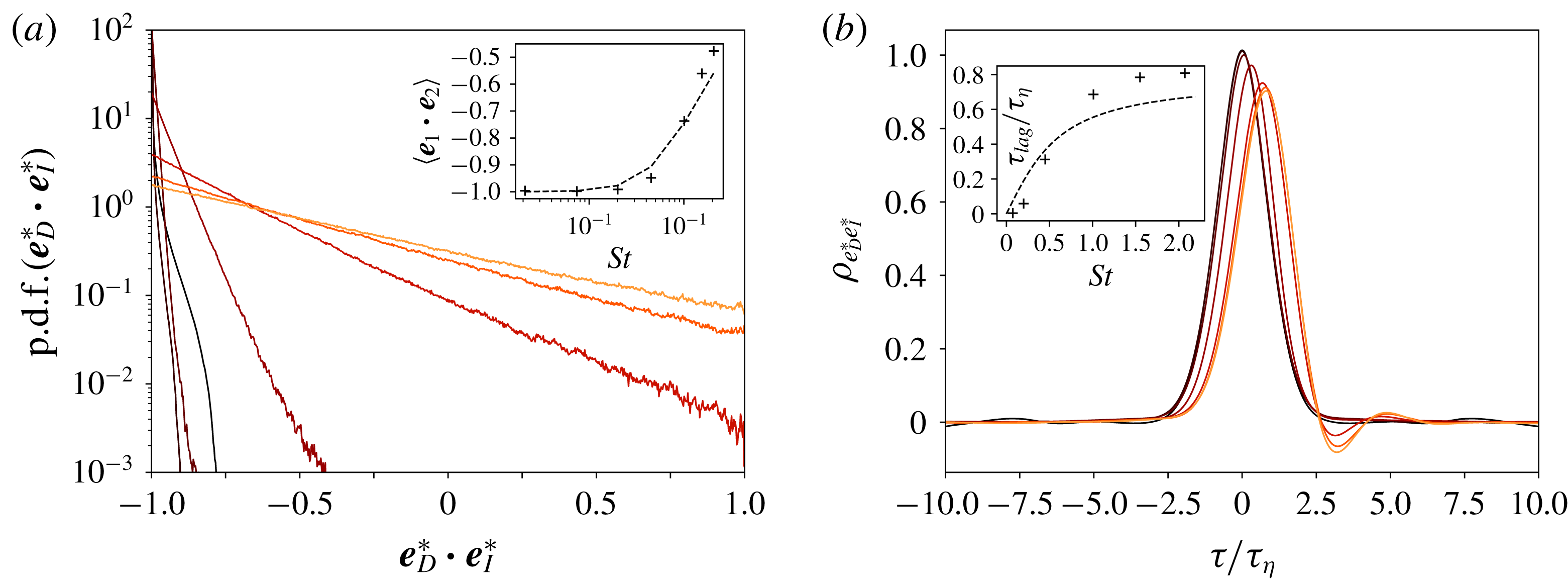
Figure 8(a) presents the evolution of the p.d.f. of the relative orientation between the two forces $\cos \unicode[STIX]{x1D703}^{\ast }=\boldsymbol{e}_{D}^{\ast }\boldsymbol{\cdot }\boldsymbol{e}_{I}^{\ast }$ , obtained from numerical integration of the stochastic orientation model (4.8)–(4.11) (and setting $D_{t}\overline{\boldsymbol{u}}_{f}=0$ in (4.8)). We clearly observe that at small Stokes number the model predicts an anti-alignment between the two orientation vectors while their relative orientation becomes more isotropic when the Stokes number increases. This behaviour is in agreement with the statistics computed from the DNS (see figure 5 b), although the p.d.f. from the DNS present a more stretched tail. It is also confirmed in the inset of figure 8(a) that the proposed stochastic model gives the correct evolution of the average relative orientation with the Stokes number, since as in the DNS case $\langle \cos \unicode[STIX]{x1D703}^{\ast }\rangle$ follow the relation (3.8). The cross-correlation between $\boldsymbol{e}_{D}^{\ast }$ and $\boldsymbol{e}_{I}^{\ast }$ is also presented in figure 8(b). The behaviour of the DNS observed in figure 6 can be qualitatively reproduced by the stochastic model with an increase of the time lag with the Stokes number.

Figure 8.

(a) The p.d.f.s of $\boldsymbol{e}_{I}^{\ast }\boldsymbol{\cdot }\boldsymbol{e}_{D}^{\ast }$ for $St=0.02$ , 0.074, 0.20, 0.45, 1.01, 1.55 and 2.07 (from black to red, respectively) as obtained from model (4.8)–(4.11). The inset is the evolution of $\langle \boldsymbol{e}_{D}^{\ast }\boldsymbol{\cdot }\boldsymbol{e}_{I}^{\ast }\rangle$ with $St$ as given by the stochastic model, and comparison with the relation (3.8). (b) Cross-correlation between $\boldsymbol{e}_{D}^{\ast }$ and $\boldsymbol{e}_{I}^{\ast }$ obtained from the model (4.8)–(4.11). The inset is the evolution of the time lag between $\boldsymbol{e}_{D}^{\ast }$ and $\boldsymbol{e}_{I}^{\ast }$ against $St$ , and comparison with $\unicode[STIX]{x1D70F}_{\unicode[STIX]{x1D702}}(\unicode[STIX]{x1D6FD}-1)^{-1}\tan ^{-1}((\unicode[STIX]{x1D6FD}-1)St)$ .

The resolved contribution in (4.1) is obtained from a spatially and temporarily averaged version of (2.1). The spatial average arises from substituting the actual velocity field $\boldsymbol{u}_{f}$ to the coarse-grained velocity field $\overline{\boldsymbol{u}}_{f}$ in this equation. In addition, a temporal filter is also explicitly applied to prevent the term $\overline{\boldsymbol{a}}$ developing high frequencies that would correlate with the residual term. Removing the frequencies above $1/\unicode[STIX]{x1D70F}_{\unicode[STIX]{x1D6E5}}$ results in the following expression for $\overline{\boldsymbol{a}}$ (see also Gorokhovski & Zamansky Reference Gorokhovski and Zamansky2018):

(4.12) $$\begin{eqnarray}\overline{\boldsymbol{a}}=-\frac{\boldsymbol{u}_{b}-\overline{\boldsymbol{u}}_{f}}{\max (\unicode[STIX]{x1D70F}_{b},\unicode[STIX]{x1D70F}_{\unicode[STIX]{x1D6E5}})}+\unicode[STIX]{x1D6FD}\frac{\text{D}\overline{\boldsymbol{u}}_{f}}{\text{D}t},\end{eqnarray}$$

where $D_{t}\overline{\boldsymbol{u}}_{f}=\unicode[STIX]{x2202}_{t}\overline{\boldsymbol{u}}_{f}+\overline{\boldsymbol{u}}_{f}\boldsymbol{\cdot }\unicode[STIX]{x1D735}\overline{\boldsymbol{u}}_{f}$ is the fluid total acceleration computed from the coarse mesh. Note that one does not have to necessarily consider the coupling with the LES to use the proposed model. Indeed, by considering the limit $\unicode[STIX]{x1D6E5}\rightarrow L$ , $L$ being the integral length scale, the term $\overline{\boldsymbol{a}}$ vanishes and (4.1) becomes $\boldsymbol{a}_{b}=\boldsymbol{a}^{\ast }$ . As well, in this limit one can replace $\unicode[STIX]{x1D700}_{\unicode[STIX]{x1D6E5}}(t)$ in (4.7) by the constant value $\langle \unicode[STIX]{x1D700}\rangle$ . For example, one can estimate the Reynolds number dependence for the intermittency correction in (3.5) from the moments of a log-normal variable, to be $\langle \boldsymbol{a}_{b}^{2}\rangle /a_{\unicode[STIX]{x1D702}}^{2}\propto \exp (3/8\,\unicode[STIX]{x1D70E}^{2})=Re_{\unicode[STIX]{x1D706}}^{0.135}$ , as proposed by Yeung et al. (Reference Yeung, Pope, Lamorgese and Donzis2006).

In order to assess the approach (4.1) as well as the stochastic model proposed in (4.6)–(4.11), we present a comparison of the statistics of the bubble dynamics obtained from the DNS, the standard LES (without modelling of the residual bubble acceleration i.e. setting $\boldsymbol{a}^{\ast }=0$ in (4.1)), and the LES with the proposed model. All the comparisons are made for $Re_{\unicode[STIX]{x1D706}}\approx 200$ and three resolutions are used for the LES ( $32^{3}$ , $48^{3}$ and $64^{3}$ ) while the resolution of the DNS is $1024^{3}$ . The details of the LES are given in § 2.

We first present in figure 9(a) the evolution of the bubble acceleration variance with the Stokes number. We observe that the standard LES largely underestimates the bubble acceleration variance compared to the DNS. As expected the discrepancy increases as the mesh resolution is made coarser. This points out that the residual term in (4.1) is dominant. In contrast, the LES supplemented by the stochastic modelling is in very good agreement with the DNS. Moreover, with the stochastic model, the LES presents a very small dependence on the grid resolution. This confirms that the effects of the unresolved small scales of the flow are correctly accounted for by the model.

Figure 9(b) presents the p.d.f. of the bubble acceleration for the various Stokes numbers. It is seen that the standard LES predicts p.d.f.s that depart significantly from the DNS and remain much closer to the Gaussian distribution. On the other hand, the p.d.f.s from the LES with the stochastic model overlap very well with the p.d.f.s of the DNS over the whole range of Stokes numbers considered here. This shows that the intermittent behaviour of the bubble acceleration can be reproduced with the proposed stochastic model.

Figure 9.

(a) Bubble acceleration variance normalized by the Kolmogorov acceleration ( $a_{\unicode[STIX]{x1D702}}^{2}$ ) versus Stokes number in logarithm scale. Open symbols are LES with the proposed model; filled symbols are LES without model; for the three meshes we have $32^{3}$ (circles), $48^{3}$ (triangles) and $64^{3}$ (diamonds). Comparison with our DNS blue stars. (b) The p.d.f. of the bubble acceleration normalized by its variance for $St=0.02$ , 0.074, 0.20, 0.45, 1.01, 1.55 and 2.07 (shifted upward by one decade each other, respectively). The DNS is a dashed black line, LES with the proposed model for $64^{3}$ is a solid red line and LES without model for $64^{3}$ is a blue dashed line.

We consider in figure 10 the autocorrelation of the acceleration component. As illustrated for $St=1$ , the decorrelation of the acceleration is much slower from the LES than from the DNS. This is expected since the decorrelation of the acceleration component is attributed to the small-scale motions of the flow which are discarded in the LES. For the LES supplemented with the model the evolution of the correlation coefficient presents qualitative agreement with the DNS. This behaviour is confirmed in the inset of figure 10 which presents the correlation time, defined as the zero crossing time, against the Stokes number. It is observed that the correlation times obtained from the DNS and from the LES with the model both remain of the order of $\unicode[STIX]{x1D70F}_{\unicode[STIX]{x1D702}}$ , whereas the standard LES predicts a much larger correlation time. We observe that the orientation model plays an essential role in obtaining an accurate estimation of the decorrelation time, and it is likely that an improvement of the model given by (4.8)–(4.11) could reduce the small discrepancies seen between the LES using the model and the DNS.

Figure 10.

Autocorrelation of the bubble acceleration for $St=0.07$ . The DNS is a solid black line, LES with model for $64^{3}$ is a dashed red line and LES without model for $64^{3}$ is a dot-dashed black line. The inset is the evolution of the corresponding integral time scale normalized by the Kolmogorov time with the Stokes number. The DNS are circles, LES with the proposed model are stars, LES without model are crosses. The mesh size for the LES is $64^{3}$ .

To evaluate the capability of the stochastic approach to accurately reproduce the time structure of the bubble velocity, we report in figure 11 the statistic of the velocity increments along the bubble trajectory. For that, we consider the structure function for a component of the bubble velocity $S_{q}(\unicode[STIX]{x1D70F})=\langle (u_{b,x}(t+\unicode[STIX]{x1D70F})-u_{b,x}(t))^{q}\rangle$ . In figure 11(a) we present the evolution of the variance of the velocity increments, $S_{2}$ , with the time shift. The results from the LES with the proposed model follow very well those obtained from the DNS, whereas with the standard LES, the variance of the velocity increments is largely underestimated. Moreover, we observe that with the stochastic model the LES can reproduce the inertial range as observed from the DNS contrary to the standard LES. Figure 11(b) shows the evolution of the flatness of the bubble velocity increments, $S_{4}/S_{2}^{2}$ . We see that with the standard LES the flatness remains close to its Gaussian value at all time shifts. In contrast, the LES with the proposed model gives an evolution of the flatness in agreement with the DNS, presenting a value close to 3 at large $\unicode[STIX]{x1D70F}$ and a significant increase with a reduction of the time shift. One can then conclude that intermittency effects associated with the small scales of the velocity field can be captured by the LES supplemented by the proposed model. Note that in figure 11 we have presented the evolution of the structure function for $St=1$ , but the same behaviour is obtained for the other values of Stokes number considered here.

Figure 11.

(a) Evolution of the second-order Lagrangian structure function with the time lag. (b) Evolution of the flatness of the Lagrangian velocity increments with the time lag. Comparison between the DNS (solid blue line), the Standard LES (black dot-dashed lines) and LES with the proposed model (dashed red lines). For both figures, for $St=0.02$ , the mesh size for the LES is $64^{3}$ .

We present in figure 12, $\langle \boldsymbol{a}_{b}^{2}|\unicode[STIX]{x1D700}_{\ast }\rangle$ , the variance of the bubble acceleration conditioned on the value of the instantaneous value of the dissipation rate $\unicode[STIX]{x1D700}_{\ast }$ estimated from the stochastic model (4.7). It is observed that similar to the DNS results reported in the figure 7, the bubble acceleration from the LES with the model increases as $\unicode[STIX]{x1D700}_{\ast }^{3/2}$ for large values of the dissipation rate, and is independent on $\unicode[STIX]{x1D700}_{\ast }$ for the small values of the latter. This behaviour shows that the acceleration of the bubbles in the weakly dissipative regions can be computed by the resolved contribution $\overline{\boldsymbol{a}}_{b}$ , indicating the influence of the large-scale sweeps, while the largest fluctuation of the acceleration are correctly estimated with the stochastic model.

Figure 12.

Variance of the total bubble acceleration $\boldsymbol{a}_{b}=\overline{\boldsymbol{a}}_{b}+\boldsymbol{a}_{\ast }$ conditioned on the stochastic value of the dissipation rate $\unicode[STIX]{x1D700}_{\ast }$ obtained from the LES with the stochastic model (black line) and comparison with the bubble acceleration variance conditioned on the local dissipation rate obtained from the DNS (red line), with $St=0.02$ and a mesh size of $48^{3}$ for the LES.