

Introduction
Due to soil variability, within-field yield differences of up to 10-fold are common in vineyards (Bramley and Lamb Reference Bramley and Lamb2003). Similar differences in canopy surface and density drive variable vine water demand; however, variable rate irrigation technology has not been developed for permanent crops. Vineyards have been divided in a small number of management zones and irrigated accordingly in Australia (McClymont et al., Reference McClymont, Goodwin, Mazza, Baker, Lanyon, Zerihun, Chandra and Downey2012; Proffitt and Pearce, Reference Proffitt and Pearce2004) and Spain (Bellvert et al., Reference Bellvert, Marsal, Mata and Girona2012; Martínez-Casasnovas et al., Reference Martínez-Casasnovas, Vallés Bigorda and Ramos2009). Likewise, in some drip-irrigated California vineyards differential watering rates are empirically achieved by increasing or decreasing the number of irrigation tubes or emitters per vine. However, the rates achieved with zonal irrigation are hard to modify once in place and in some cases the length and frequency of irrigation periods cannot be controlled independently for each zone because all the emitters are connected to the same circuit and a single pump.
The main objective of the study described herein was to develop a modular, proof-of-concept variable rate irrigation (VRDI) system prototype, operate it using NDVI and an energy balance model based on remotely sensed data and differentially deliver water to 140 equally sized irrigation zones to control vine growth and yield.
Materials and methods
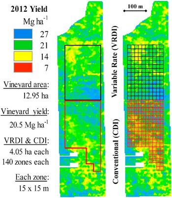
A highly variable, hand-pruned, drip-irrigated, 17-year old Cabernet Sauvignon vineyard, for which yield had previously been mapped during the 2012 harvest, was selected for this study. The 12.5 ha block is located north of Lodi, California (38°21'13.60''N/121°15'1.80''W; elevation 21 meters). Local average precipitation is 500 mm occurring mostly during winter. The VRDI study was set up in a 4.05 ha rectangular section that included the full range of yields seen in the rest of the block according to the 2012 yield map (Figure 1). The perimeter of the VRDI section was aligned with the 30×30 m pixels of the Landsat scene covering the site, and each pixel was further divided into four 15×15 m quadrants, each one defining an independent irrigation zone. This grid resulted in a rectangle containing 140 irrigation zones, each containing 40 or 50 vines. A second 4.05 ha grid, was setup adjacent to the south edge of the VRDI area to extract “control” spatial data and was denominated conventional drip irrigation (CDI).
VRDI and CDI location and grids in the vineyard.

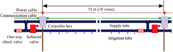
Details of the VRDI prototype design and operation can be found in Sanchez et al. (Reference Sanchez, Mendez-Costabel, Sams, Morgan, Dokoozlian, Klein, Hinds, Hamann, Claassen and Lew2014). Briefly, the system consisted of a variable flow submersible pump, underground pipes, power and communication wiring, solenoid valves, flow meters, and a large panel holding several enclosures for power and electronics components as well as the central computer, an antenna and a wireless modem for remote access and control. As shown in Figure 2, water was delivered through two PVC irrigation tubes (1.78 cm outside diameter) which ran parallel on a vertical plane 15 cm apart from each other. The upper tube was fastened to a wire running along the vine row at a height of 60 cm. The lower tube ran along with the primary irrigation system tube and both were held by a second wire at a height of 45 cm. The two wires were fastened to the vine support stakes and both tubes were connected to each other through an “H” PVC assembly, in place every 10 vine spaces or 15 m. Only the lower hose had drip emitters, two per vine. Independent irrigation of the each of the four or five 10-vine sections of each irrigation zone was achieved with the opening of a solenoid valve on one end of the irrigation section and a one-way check valve on the other end which allowed water to flow out in one direction when the solenoid valve was open but not in the opposite direction when it was closed. A small enclosure (controller box in Figure 2) held by a metal stake contained an electronic control board as well as power and communication wiring.
Diagram of the water delivery components in each irrigation section.

The primary irrigation system was kept in place as backup and for uniform application of liquid fertilizers as needed. Irrigation of the 140 zones was controlled by a computer network with a single master coordinating operation communicating through a MODBUS-based protocol (Modbus.org, 2006). Remote desktop operations, including uploading the weekly irrigation schedules and troubleshooting, were accomplished via cellular link with the central computer and its modem.
Weekly irrigations were scheduled for each zone using the equation: ETc=(ETref)*(Kc)*(Km), where ETc=crop evapotranspiration, ETref=reference crop evapotranspiration, Kc=crop coefficient (increases with canopy development), and Km=management factor. ETref was obtained from the nearest California Irrigation Management Information System weather station (CIMIS, 2017). Kc was calculated by multiplying the NDVI of each zone by a factor of 1.1. This factor, calculated once at the start of irrigations over many mature vineyards and varieties, is the ratio of NDVI and a Kc calculated with the METRIC (Mapping EvapoTranspiration at high Resolution with Internalized Calibration) energy balance model (Allen et al., Reference Allen, Tasumi and Trezza2007). METRIC calculates evapotranspiration (ET) as a residual of the surface energy balance:
 $$LE\,{\equals}\,R_{n} -G-H$$
where LE is latent energy consumed by ET (W⋅m −2 ); Rn is net radiation; G is sensible heat flux conducted into the ground (W⋅m −2 ); and H=sensible heat flux convected to the air (W⋅m −2 ).
METRIC is applied using multispectral Landsat satellite imagery and weather data (CIMIS, 2017). The primary output is actual evapotranspiration at the pixel scale. Ideally METRIC would be calculated on a weekly basis however it was necessary to use the ratio described above and weekly NDVI values as it was much less time demanding. Multispectral band reflectance data was obtained from Landsat 8 and 7 and processed using one the METRIC modules to atmospherically correct the data and calculate NDVI. While the calculated irrigation amounts were proportional to the vigor (NDVI) of each irrigation zone, a management factor (Km) varying between 0 and 1.2 was imposed based either on yield (2012 yield map) or on the current NDVI values for each zone. The objective here was to differentially manipulate vigor and yield according to vineyard variability. Zones with higher stress values (low vine vigor or yield) received more water. Proportionally higher Km values were applied to the low yield zones in 2014 than in 2013 and 2015. In 2015 the Km was continuously adjusted solely based on vine vigor as estimated by the Landsat-derived NDVI. The remaining vineyard was irrigated using the primary system at a uniform rate, with Km values at the discretion of the vineyard manager.
Yield was measured spatially at harvest (Bramley and Williams, Reference Bramley and Williams2001) with yield monitors (ATV, Joslin, Australia) installed on several models of over-the-row trunk-shaking mechanical harvesters. Harvest data were cleaned-up with a script written in RStudio software (RStudio Inc., Boston, MA, USA, 2015) to convert mass flow units into Mg ha−1, eliminate outliers, and normalize harvesters. Data were then transferred into VESPER Version 1.62 (Minasny et al., 2005) for kriging to 3×3 m resolution. Yield map values were normalized to zero mean and unit variance for multi-year comparisons.
Irrigation treatment effects were analyzed using the 3×3 m data or their average for each 15×15 m irrigation zone. Variogram parameters were obtained from VESPER and constrained to a range of 100 m to calculate spatial statistics for yield and NDVI. Qualitative spatial indices included the Cambardella index, CI (Cambardella et al., Reference Cambardella, Moorman, Novak, Parkin, Karlen, Turco and Konopka1994), and the mean correlation distance, MCD (Han et al., 1994). CI values were assessed as less than 25 indicating strong spatial dependency, 25–75 indicating moderate spatial dependency, and greater than 75 indicating weak spatial dependency. Conversely, higher MCD values were equated to greater spatial structure.
Applied irrigation amounts were monitored continuously in the VRDI and CI systems using inline flow meters and pressure switches. Water use efficiency (WUE) was calculated as kg of fruit harvested per mm irrigation water applied.
Results and discussion
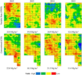
Figure 3 shows the normalized yield maps of VRDI and CDI for 2012 (before installation) and 2013 through 2015 (after installation). Due to the natural variation in bud fruitfulness, whole-vineyard yield was high in 2012 and 2014 and low in 2013 and 2015. However, yields under VRDI were on average 10% higher than under CDI in all three years under variable rate irrigation. The general spatial distribution pattern of high and low yielding areas did not change under CDI in all four years (Figure 3, lower panel). On the other hand, the VRDI strategies caused significant changes to spatial variability. Yield spatial variability decreased in 2013 and 2015. In 2014, by selectively increasing management factors in the low vigor/yield irrigation zones, VRDI reversed the relative spatial distribution of yield compared to 2012.
Normalized yield maps (zero mean and unit variance) for VRDI and CDI in 2012 (before the VRDI system was installed), 2013, 2014 and 2015.

The increase in yield under VRDI occurred in the irrigation zones where higher Km values were used and which had low vigor and yield in 2012. The yield increase was due mostly to an increase in berry size (results not shown). It is expected that if these low vigor vines continue under higher irrigation (higher Km values) for several years, eventually they will increase in capacity and in fruitfulness, leading to increased berries per cluster and clusters per vine.
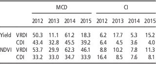
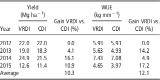
Spatial structure of yield and NDVI, given by MCD and CI, varied according to the results described above, being high in 2012 and 2014 and low in 2013 and 2015 (Table 1). Remarkably, these yield differences were achieved without decreasing WUE. In fact, WUE was on average higher in VRDI than CDI for all three years (Table 2).
Spatial structure of yield and NDVI for VRDI and CDI in the four years of the study

MCD=Mean Correlation Distance; CI=Cambardella Index.
Average yield and WUE of VRDI and CDI in the four years of the study

The VRDI prototype not only fulfilled very well its proof of concept but also performed without major problems during its three years of operation. Due to the high number of components, it was expensive to operate and maintain but served as the template for a much less complex and simpler to operate system currently under testing for commercialization.
Conclusions
A low-volume, VRDI prototype was successfully designed and deployed in a wine grape vineyard in California and irrigations were scheduled weekly based on NDVI derived from Landsat images and differentially applied management factors. Vine growth was effectively and immediately manipulated with variable rate irrigation. Yield was increased during the three seasons by an average of 10% with up to 17% gain in water use efficiency.
This first VRDI prototype constitutes new precision viticulture technology for the vineyard of the future, in which a flexible, modular variable rate water delivery system is coupled with satellite data for farming at the pixel level. This system can be used to irrigate each zone according to vine size without altering natural variability or to apply an irrigation management factor to low vigor areas in order to increase vine size and yield and decrease vineyard variability.
Acknowledgements
Alan Claassen and David Lew, formerly at IBM Systems and Technology Group, San Jose, CA; James Taylor, Newcastle University, UK; Ernie & Jeff Dosio, Pacific Agrilands, Lodi, CA; Bernd Kleinlagel, Advanced Technology Viticulture, Australia.