





%20--%3e%3c!DOCTYPE%20svg%20PUBLIC%20'-//W3C//DTD%20SVG%201.0//EN'%20'http://www.w3.org/TR/2001/REC-SVG-20010904/DTD/svg10.dtd'%3e%3csvg%20version='1.0'%20id='Layer_1'%20xmlns='http://www.w3.org/2000/svg'%20xmlns:xlink='http://www.w3.org/1999/xlink'%20x='0px'%20y='0px'%20width='64px'%20height='64px'%20viewBox='5.5%20-3.5%2064%2064'%20enable-background='new%205.5%20-3.5%2064%2064'%20xml:space='preserve'%3e%3cg%3e%3ccircle%20fill='%23FFFFFF'%20fill-opacity='0'%20cx='37.785'%20cy='28.501'%20r='28.836'/%3e%3cpath%20fill='%23595959'%20d='M37.441-3.5c8.951,0,16.572,3.125,22.857,9.372c3.008,3.009,5.295,6.448,6.857,10.314%20c1.561,3.867,2.344,7.971,2.344,12.314c0,4.381-0.773,8.486-2.314,12.313c-1.543,3.828-3.82,7.21-6.828,10.143%20c-3.123,3.085-6.666,5.448-10.629,7.086c-3.961,1.638-8.057,2.457-12.285,2.457s-8.276-0.808-12.143-2.429%20c-3.866-1.618-7.333-3.961-10.4-7.027c-3.067-3.066-5.4-6.524-7-10.372S5.5,32.767,5.5,28.5c0-4.229,0.809-8.295,2.428-12.2%20c1.619-3.905,3.972-7.4,7.057-10.486C21.08-0.394,28.565-3.5,37.441-3.5z%20M37.557,2.272c-7.314,0-13.467,2.553-18.458,7.657%20c-2.515,2.553-4.448,5.419-5.8,8.6c-1.354,3.181-2.029,6.505-2.029,9.972c0,3.429,0.675,6.734,2.029,9.913%20c1.353,3.183,3.285,6.021,5.8,8.516c2.514,2.496,5.351,4.399,8.515,5.715c3.161,1.314,6.476,1.971,9.943,1.971%20c3.428,0,6.75-0.665,9.973-1.999c3.219-1.335,6.121-3.257,8.713-5.771c4.99-4.876,7.484-10.99,7.484-18.344%20c0-3.543-0.648-6.895-1.943-10.057c-1.293-3.162-3.18-5.98-5.654-8.458C50.984,4.844,44.795,2.272,37.557,2.272z%20M37.156,23.187%20l-4.287,2.229c-0.458-0.951-1.019-1.619-1.685-2c-0.667-0.38-1.286-0.571-1.858-0.571c-2.856,0-4.286,1.885-4.286,5.657%20c0,1.714,0.362,3.084,1.085,4.113c0.724,1.029,1.791,1.544,3.201,1.544c1.867,0,3.181-0.915,3.944-2.743l3.942,2%20c-0.838,1.563-2,2.791-3.486,3.686c-1.484,0.896-3.123,1.343-4.914,1.343c-2.857,0-5.163-0.875-6.915-2.629%20c-1.752-1.752-2.628-4.19-2.628-7.313c0-3.048,0.886-5.466,2.657-7.257c1.771-1.79,4.009-2.686,6.715-2.686%20C32.604,18.558,35.441,20.101,37.156,23.187z%20M55.613,23.187l-4.229,2.229c-0.457-0.951-1.02-1.619-1.686-2%20c-0.668-0.38-1.307-0.571-1.914-0.571c-2.857,0-4.287,1.885-4.287,5.657c0,1.714,0.363,3.084,1.086,4.113%20c0.723,1.029,1.789,1.544,3.201,1.544c1.865,0,3.18-0.915,3.941-2.743l4,2c-0.875,1.563-2.057,2.791-3.541,3.686%20c-1.486,0.896-3.105,1.343-4.857,1.343c-2.896,0-5.209-0.875-6.941-2.629c-1.736-1.752-2.602-4.19-2.602-7.313%20c0-3.048,0.885-5.466,2.658-7.257c1.77-1.79,4.008-2.686,6.713-2.686C51.117,18.558,53.938,20.101,55.613,23.187z'/%3e%3c/g%3e%3c/svg%3e)
%20--%3e%3c!DOCTYPE%20svg%20PUBLIC%20'-//W3C//DTD%20SVG%201.0//EN'%20'http://www.w3.org/TR/2001/REC-SVG-20010904/DTD/svg10.dtd'%3e%3csvg%20version='1.0'%20id='Layer_1'%20xmlns='http://www.w3.org/2000/svg'%20xmlns:xlink='http://www.w3.org/1999/xlink'%20x='0px'%20y='0px'%20width='64px'%20height='64px'%20viewBox='5.5%20-3.5%2064%2064'%20enable-background='new%205.5%20-3.5%2064%2064'%20xml:space='preserve'%3e%3cg%3e%3ccircle%20fill='%23FFFFFF'%20fill-opacity='0'%20cx='37.637'%20cy='28.806'%20r='28.276'/%3e%3cg%3e%3cpath%20fill='%23595959'%20d='M37.443-3.5c8.988,0,16.57,3.085,22.742,9.257C66.393,11.967,69.5,19.548,69.5,28.5c0,8.991-3.049,16.476-9.145,22.456%20C53.879,57.319,46.242,60.5,37.443,60.5c-8.649,0-16.153-3.144-22.514-9.43C8.644,44.784,5.5,37.262,5.5,28.5%20c0-8.761,3.144-16.342,9.429-22.742C21.101-0.415,28.604-3.5,37.443-3.5z%20M37.557,2.272c-7.276,0-13.428,2.553-18.457,7.657%20c-5.22,5.334-7.829,11.525-7.829,18.572c0,7.086,2.59,13.22,7.77,18.398c5.181,5.182,11.352,7.771,18.514,7.771%20c7.123,0,13.334-2.607,18.629-7.828c5.029-4.838,7.543-10.952,7.543-18.343c0-7.276-2.553-13.465-7.656-18.571%20C50.967,4.824,44.795,2.272,37.557,2.272z%20M46.129,20.557v13.085h-3.656v15.542h-9.944V33.643h-3.656V20.557%20c0-0.572,0.2-1.057,0.599-1.457c0.401-0.399,0.887-0.6,1.457-0.6h13.144c0.533,0,1.01,0.2,1.428,0.6%20C45.918,19.5,46.129,19.986,46.129,20.557z%20M33.042,12.329c0-3.008,1.485-4.514,4.458-4.514s4.457,1.504,4.457,4.514%20c0,2.971-1.486,4.457-4.457,4.457S33.042,15.3,33.042,12.329z'/%3e%3c/g%3e%3c/g%3e%3c/svg%3e)
1. Introduction
1.1. Characteristics of the flow around spheroids
Slender bodies have been widely studied for aerospace (fuselage) and marine engineering (underwater vehicle) applications. Among them, the prolate spheroid has been a commonly studied geometry, which can produce a variety of flows in the wake, including variations as an inclination angle,  $\theta$, (negative pitch) varies from zero.
When  $\theta = 0^\circ$, a streamlined body has a relatively small recirculating, or wake region, commensurate with the low drag per unit volume. As noted by Ortiz-Tarin, Nidhan & Sarkar (Reference Ortiz-Tarin, Nidhan and Sarkar2021), unlike bluff-body wakes, where the near wake can be strongly influenced by vortex shedding (Johansson & George Reference Johansson and George2006), the flow immediately behind a slender body is characterised by axisymmetric turbulence where the near wake is quasi-parallel, with broadband turbulence (Jiménez, Hultmark & Smits Reference Jiménez, Hultmark and Smits2010; Kumar & Mahesh Reference Kumar and Mahesh2018).
With increasing  $\theta$, the leeward separation line moves forward, closer to the leading edge, and at sufficiently high
 $\theta$, the flow wraps around the body, rolling up into a separation vortex on both sides (Wang et al. Reference Wang, Zhou, Hu and Harrington1990; Fu et al. Reference Fu, Shekarriz, Katz and Huang1994; Xiao et al. Reference Xiao, Zhang, Huang, Chen and Fu2007; Jiang et al. Reference Jiang, Gallardo, Andersson and Okulov2016). Such separation vortices were observed in experiments on a 6 : 1 spheroid at
 $\theta =10^\circ$ and
 ${\textit {Re}}=3.5 \times 10^5$, consistent with the roll-up of a pair of vortex sheets that originated from the body (Fu et al. Reference Fu, Shekarriz, Katz and Huang1994). The strong primary separation vortices can induce counter-rotating, secondary vortices in the boundary layer beneath, and further, smaller separation vortices can also be formed (Fu et al. Reference Fu, Shekarriz, Katz and Huang1994; Chesnakas & Simpson Reference Chesnakas and Simpson1997; Wetzel, Simpson & Chesnakas Reference Wetzel, Simpson and Chesnakas1998). Certain details of the separation and reattachment of the primary and secondary vortices were noted in a hybrid Reynold-averaged Navier–Stokes/large eddy simulation (RANS/LES) of a 6 : 1 spheroid at
 $\theta = 20^\circ$ and
 ${\textit {Re}} = 7 \times 10^5$ (Xiao et al. Reference Xiao, Zhang, Huang, Chen and Fu2007).
The topology of the separated vortex wake from a slender body at incidence depends on both Re and  $\theta$. Nelson et al. (Reference Nelson, Corke and Matsuno2006) classified the flows into four regimes, depending on the wake geometry: vortex-free flow, symmetric vortex shedding, asymmetric vortex shedding and unsteady vortex wakes. Although this classification is based on the wakes of a slender body with a pointed nose and a blunt tail (figure 1b), similar variations of vortex wakes were observed in other inclined slender geometries, such as a cylinder with a hemispherical nose (
 ${AR} = 8$) (figure 1c) (Hoang & Telionis Reference Hoang and Telionis1991) and a prolate spheroid (
 ${AR} = 6$) (figure 1a) (Jiang et al. Reference Jiang, Gallardo, Andersson and Okulov2016). The separation vortices can interact with the drag wake, altering the near-wake dynamics and energetics. Delay in the formation and migration of separation lines for unsteady flows and high inclination angles may lead to further different flow topologies (Wetzel et al. Reference Wetzel, Simpson and Chesnakas1998).
Illustrations of slender body geometries tested in previous literature: (a) a prolate spheroid (Jiang et al. Reference Jiang, Gallardo, Andersson and Okulov2016); (b) a body with a pointed nose and a blunt tail (Nelson, Corke & Matsuno Reference Nelson, Corke and Matsuno2006); (c) a cylinder with a hemispherical nose (Hoang & Telionis Reference Hoang and Telionis1991). The body is characterised by the aspect ratio  ${AR} = L/D$, the angle of attack
 $\theta$ with respect to the flow direction
 $U$.

As the strength of the separation vortices increases with increasing  $\theta$, unstable separation vortices (Hoang & Telionis Reference Hoang and Telionis1991) or asymmetric separation can occur, as observed in the numerical simulation of a 6 : 1 spheroid at
 $\theta =10^\circ$ and
 ${\textit {Re}}=3.5 \times 10^5$ (Strandenes et al. Reference Strandenes, Jiang, Pettersen and Andersson2019) and in experiments on a DARPA SUBOFF model for
 $\theta = 8^\circ$ and
 ${\textit {Re}}_L = 2.4 \times 10^6$ (
 ${\textit {Re}}_D = 2.8 \times 10^5$) by Ashok, Van Buren & Smits (Reference Ashok, Van Buren and Smits2015). When there is an imbalance in the circulation of counter-rotating vortex pair, the weaker vortex wraps around the stronger one, increasing the asymmetry in the wake and eventually resulting in annihilation of the weaker vortex.
1.2. Spheroids in a stratified ambient
In a vertical, uniform density gradient,  ${\rm d}\rho /{\rm d}z$, there is a natural resonant frequency
 $N = [(-g/\rho _0) ({\rm d}\rho /{\rm d}z)]^{1/2}$ as fluid elements oscillate around their neutral density
 $\rho _0$. This gives a buoyancy time scale,
 $1/N$, and the ratio of this time scale to an advective time scale
 $D/U$ yields an internal Froude number,
 ${\textit {Fr}} = 2U/ND$. Here we use the length
 $D/2$, when maximum resonance on a half-wave cycle occurs for
 ${\textit {Fr}} = 1$. In this formulation,
 $N$ has units of
 ${\rm rad}\ {\rm s}^{-1}$. Definitions of
 ${\textit {Fr}}$ in the literature vary by factors of
 $2{\rm \pi}$ when
 $N$ is expressed as a cycle frequency in /s, and the choice of
 $D$ or
 $D/2$ is not universal. The Reynolds number is based on
 $D$ and the travel speed,
 $U$,
 ${\textit {Re}}= UD/\nu$, where
 $\nu$ is the kinematic viscosity.
Early work on slender bodies in a stratified environment was driven strongly by naval applications, so many experiments focused on self-propelled configurations. Schooley & Stewart (Reference Schooley and Stewart1962) used dye to estimate horizontal and vertical growth rates of the wake behind a self-propelled body. The body itself was an unfaired cylindrical motor ( ${AR} = L/D \approx 2$) that was self-propelled in the 23D central section of a tow tank. The wake width grew faster than the height, which was constrained by buoyancy forces. The single rotating propeller of
 $d = 0.82D$ strongly mixed the fluid in the near wake, and so was born the idea that the unstable neutral density tube in the midst of a stratified background would collapse and shrink under the influence of buoyancy. This readjustment of the wake was then associated with generation of internal gravity waves, whose surface signature was measured through the displacements of dye spots on the free surface. Lin & Pao (Reference Lin and Pao1979) reviewed the literature for stratified wakes, including those of axisymmetric slender bodies. All the quantitative data in this paper are for the self-propelled configuration. Though a significant drop in wake height is not evident from the data, growth in the vertical direction halts at approximately the same critical
 $Nt$ where the wake width was seen to increase at a faster rate. It was noted that the reduction in wake height was much smaller than originally reported by Schooley & Stewart (Reference Schooley and Stewart1962), perhaps because their body was not slender, and/or the wake was over-thrusted.
In oceans,  $N$ is a small number, of the order of
 $10^{-3}$, and
 ${\textit {Fr}}$ tends to be correspondingly large. The studies reviewed by Lin & Pao (Reference Lin and Pao1979) covered a range of
 ${\textit {Fr}}$ from
 $565/{\rm \pi}$ to
 $65/{\rm \pi}$ when the initial buoyancy constraints are weak. In a decaying wake,
 $U$ decreases while characteristic length scales initially increase, so a limit will be reached when a local
 ${\textit {Fr}}$ is of order one, as discussed in some detail by numerous sources including Billant & Chomaz (Reference Billant and Chomaz2001), Brethouwer et al. (Reference Brethouwer, Billant, Lindborg and Chomaz2007) and de Bruyn Kops & Riley (Reference de Bruyn Kops and Riley2019). Even when initial
 ${\textit {Fr}}$ are
 $O(10^2)$, stratified flows will all reach a balance where buoyancy and inertial terms co-evolve with most kinetic energy confined to large-scale quasi-horizontal motions. Paradoxically, this regime becomes
 ${\textit {Fr}}$-independent.
The 6 : 1 prolate spheroid geometry was included in a study by Meunier & Spedding (Reference Meunier and Spedding2004) for  ${\textit {Re}}=5000$ and
 ${\textit {Fr}}=\{8,32\}$, and
 $x/D=\{10^2\unicode{x2013}10^4\}$ (
 $Nt=\{10\unicode{x2013}10^3\}$), and the wakes in this range of
 $x/D$ or
 $Nt$ did not differ from those previously studied, when rescaled as describe in the following section. Furthermore, Meunier & Spedding (Reference Meunier and Spedding2006) showed that except for the rare case of exactly
 $(\pm 2\,\%)$ momentum-less wakes, all self-propelled wakes when slightly over- or under-thrusted would have similar scaling. Again, in the late wake, there was no unique feature of streamlined or self-propelled bodies. A second characteristic feature of bluff body wakes is the emission of internal gravity waves from either the body or the wake itself. Meunier et al. (Reference Meunier, Le Dizés, Redekopp and Spedding2018) found that the amplitude of internal waves in the lee of spheres, cylinders and spheroids scales also approximately with the body drag, but there was an unexplained dependence of the wake waves on
 ${\textit {Re}}$, similar to that found in simulations by Abdilghanie & Diamessis (Reference Abdilghanie and Diamessis2013).
Investigating the effect of varying body geometry on near- and far-wakes presents formidable computational challenges. Ortiz-Tarin, Chongsiripinyo & Sarkar (Reference Ortiz-Tarin, Chongsiripinyo and Sarkar2019) employed LES to model the wake of a 4 : 1 spheroid and showed that the  ${\textit {Fr}}$ for maximum lee wave resonance scaled with the streamwise length,
 $L$. A hybrid simulation with different near- and far-wake spatial and temporal resolution by Ortiz-Tarin et al. (Reference Ortiz-Tarin, Nidhan and Sarkar2021) and Ortiz-Tarin, Nidhan & Sarkar (Reference Ortiz-Tarin, Nidhan and Sarkar2023) simulated the stratified wake of a 6 : 1 spheroid at
 ${\textit {Re}} = 10^5$ and
 ${\textit {Fr}}=\{1,5,\infty \}$, and commensurate with previous findings in high-Re, unstratified simulations (Chongsiripinyo, Pal & Sarkar Reference Chongsiripinyo, Pal and Sarkar2017), it was found that supposedly universal regimes and their differing growth and decay laws could not be fit to all cases.
1.3. The search for scaling laws
If and when profiles of mean and turbulence quantities are found to be self-similar, then the scaling of these functions can be used to test basic ideas on the mechanism of turbulence generation and evolution. At the outset, we might imagine that relationships derived and found for unstratified wakes may hold, and that there would be some point at which these relations fail, or change, as the anisotropic influence of buoyancy is felt. The classical results (Tennekes & Lumley Reference Tennekes and Lumley1972; Townsend Reference Townsend1976; George Reference George1989) for unstratified turbulent wakes predict that  $l \sim x^{1/3}$ and
 $u \sim x^{-2/3}$. Equivalent relationships of
 $l \sim x^{1/4}$ and
 $u \sim x^{-4/5}$ for self-propelled bodies (given a somewhat idealised expected mean streamwise velocity profile) were given by Tennekes & Lumley (Reference Tennekes and Lumley1972), and early experiments by Lin & Pao (Reference Lin and Pao1979) on self-propelled slender bodies reported wake widths and heights that departed from this norm at approximately
 $Nt = 1.25$, marking the beginning of a strong influence of the background density gradient. Growth in wake height ceased at that time, and decreased by approximately
 $15\,\%$ over the next
 $Nt = [1.25\unicode{x2013}6]$. Over the same interval, the wake width began to grow more rapidly, as
 $Nt^{0.4}$
Though it seems reasonable to expect that constraints in the vertical direction due to buoyancy would inhibit vertical growth rates, with a corresponding increase in horizontal dimension, that was not found in quantitative studies of towed sphere wakes (Spedding, Browand & Fincham Reference Spedding, Browand and Fincham1996) where horizontal growth rates  $L_h \sim x^{1/3}$ were unchanged even as vertical growth was inhibited. The resulting increase in wake energy density was associated with significantly lower centreline velocity decay rates, and the coherence and persistence of the late wake were related to the emergence of a regular pattern of vortices with much smaller vertical extent than horizontal.
The two configurations – one a slender, self-propelled body, the other a towed bluff body – have significant differences, and a subsequent study on the effect of body geometry on the late wake scaling showed that bluff (sphere), sharp-edged (disk, hemisphere, right circular cylinder, cube) and streamlined (6 : 1 prolate spheroid) bodies could be rescaled when a momentum length,  $D_m$, was introduced as a scale to account for the horizontal momentum flux. This scale was derived from known drag coefficients in unstratified conditions and allowed geometry-independent predictions for the evolution of a horizontal wake width,
 $L_H$, and centreline velocity,
 $U_0$:
 $$\begin{gather} \frac{L_H}{D_{m}} = 0.35 \left( \frac{x}{D_{m}}\right)^{0.35}, \end{gather}$$
 $$\begin{gather}\frac{U_0}{U}\textit{Fr}_{m}^{2/3} = 6.6 \left( Nt\right)^{-0.76}. \end{gather}$$
In the simplified self-similarity framework, at high  ${\textit {Re}}$, the velocity and length scales of turbulent, axisymmetric wakes behave as
 $u \sim x^{-2/3}$ and
 $l \sim x^{1/3}$ (Tennekes & Lumley Reference Tennekes and Lumley1972; Townsend Reference Townsend1976; George Reference George1989). Then, a local
 ${\textit {Re}}_l \sim ul \sim (x^{-2/3})(x^{1/3}) \sim x^{-1/3}$ decays in
 $x$. Meunier, Diamessis & Spedding (Reference Meunier, Diamessis and Spedding2006) showed that by imposing a Gaussian mean profile onto the momentum equation, the similarity solution then depends on three independent variables that evolve in
 $x$, the peak velocity
 $u_0$, wake width
 $L_H$ and wake height
 $L_V$. As
 $u_0$ continues to decay, the local Fr (
 ${\textit {Fr}} \sim x^{-1}$) approaches order 1 at
 $Nt \sim 2$, and buoyancy effects become increasingly influential, entering a non-equilibrium, or NEQ, regime, where the wake adjusts to the buoyancy force. The transition to NEQ is predicted to occur at
 $x/D_m = {\textit {Fr}}_m$, where
 $D_m = D\sqrt {c_D/2}$ is a momentum thickness and
 $c_D$ is the body drag coefficient. The mean wake dynamics are now determined by a balance between turbulent diffusion of momentum in the horizontal direction and viscous diffusion of momentum in the vertical direction. The combined effect in this buoyancy-controlled (BC) regime is for
 $L_H \sim x^{1/2}, L_V \sim x^0$ (initially there is no apparent increase in wake height), while
 $u_0 \sim x^{-1/2}$. Subsequently, a long-lasting quasi-two-dimensional (Q2-D) regime is reached as
 $L_V \sim x^{1/2}$ and
 $u_0 \sim x^{-3/4}$. The analysis required some quite strong assumptions on the initial Froude number (must be high) and on the negligible magnitude of vertical Reynolds stresses compared with those in the horizontal, but some simple testable predictions emerged, such as the length of the NEQ regime being proportional to
 ${\textit {Fr}}^{2/3}{\textit {Re}}$. The NEQ regime is where the animated wake adjusts to the background density gradient, in part, by emitting internal gravity waves, and so is quite important from a signature point of view.
The predictions by Meunier et al. (Reference Meunier, Diamessis and Spedding2006) agreed quite well with available laboratory and numerical experiments, though with some variance in the vertical scaling, and in the transition from BC to Q2-D regimes. Given the absence of dynamics related to vertical motions in the model, this was hardly surprising, and the interesting part was how well the phenomenology could be replicated in a very simplified framework. When examined in detail, there is abundant disagreement on the measured and expected scaling relations of both homogeneous (Bevilaqua & Lykoudis Reference Bevilaqua and Lykoudis1978; George Reference George1989; Redford, Castro & Coleman Reference Redford, Castro and Coleman2012) and stratified (Spedding Reference Spedding2002b; Brucker & Sarkar Reference Brucker and Sarkar2010; Ortiz-Tarin et al. Reference Ortiz-Tarin, Chongsiripinyo and Sarkar2019, Reference Ortiz-Tarin, Nidhan and Sarkar2023) wakes. Ortiz-Tarin et al. (Reference Ortiz-Tarin, Nidhan and Sarkar2021) highlighted some disagreements in measured scaling laws of homogeneous wakes of various geometries. Some bluff body wakes studies including sphere (Bonnier & Eiff Reference Bonnier and Eiff2002; Pal et al. Reference Pal, Sarkar, Posa and Balaras2017), disk (Nedić, Vassilicos & Ganapathisubramani Reference Nedić, Vassilicos and Ganapathisubramani2013; Chongsiripinyo & Sarkar Reference Chongsiripinyo and Sarkar2020; Nidhan et al. Reference Nidhan, Chongsiripinyo, Schmidt and Sarkar2020), dimpled sphere (Saunders et al. Reference Saunders, Frederick, Drivas and Wunsch2020; Saunders, Britt & Wunsch Reference Saunders, Britt and Wunsch2022) and fractal plate (Dairay, Obligado & Vassilicos Reference Dairay, Obligado and Vassilicos2015) reported near-wake decay rates of  $u \sim x^{-1}$ with some maintaining this rate further downstream, while others transitioned from
 $x^{-1}$ to
 $x^{-2/3}$. However, certain slender body wakes have been reported by Jiménez et al. (Reference Jiménez, Hultmark and Smits2010), Kumar & Mahesh (Reference Kumar and Mahesh2018) and Ortiz-Tarin et al. (Reference Ortiz-Tarin, Nidhan and Sarkar2021) to decay as
 $x^{-2/3}$ even early on. Redford, Lund & Coleman (Reference Redford, Lund and Coleman2015) point out that stratified wakes appear to evolve to some common state, with similar velocity and length scale evolution, which can arise from a number of different initial conditions and, at some level of detail, this seems to be the case. Models based on power laws of presumed self-similar flows are necessarily simplifications and the main question is whether the simplifications are both, at least approximately, valid and useful. As the real costs of both experiment and simulation rise steeply with increasing
 ${\textit {Re}}$ (e.g. Zhou & Diamessis Reference Zhou and Diamessis2019; Rowe, Diamessis & Zhou Reference Rowe, Diamessis and Zhou2020), having explicit, if approximate, model predictions with both
 ${\textit {Re}}$ and
 ${\textit {Fr}}$ can be valuable.
Amidst the search for general solutions, there are also some configurations that would not be expected to conform to generic wake dynamics, at least early on. Obvious examples include bodies with protrusions or plane (lifting) surfaces. One such configuration that can emerge during operations is a streamlined body at incidence, where three-dimensional (3-D) flow separation leads to strong, streamwise vortices which may then evolve separately from, or interact with, the usual drag wake.
1.4. Evolution of trailing vortices
In an homogeneous fluid, parallel counter-rotating vortices can be unstable to 3-D perturbations, including a symmetric long-wavelength instability known as the Crow instability, a symmetric and antisymmetric short-wavelength elliptical instability, and oscillatory instability for large Re (strongly deformed with large cores) (Donnadieu et al. Reference Donnadieu, Ortiz, Chomaz and Billant2009). A counter-rotating vortex pair can be characterised by the relative distance  $b$ between the vortex cores, and the vortex core radius
 $a$ (Leweke, Le Dizès & Williamson Reference Leweke, Le Dizès and Williamson2016). A stability analysis of a pair of parallel vortices predicts that the wavelength of the Crow instability is
 $\lambda =8.6b$, based upon the wavenumber with maximum amplification from the strong interaction between long waves (Crow Reference Crow1970). The elliptical instability is strongest when the two Kelvin modes (linear perturbation modes of an axisymmetric vortex, usually neutral or stable) have a similar radial structure (Leweke et al. Reference Leweke, Le Dizès and Williamson2016). At high Re, multiple elliptical instabilities emerge leading to a transient turbulent flow. In a stratified fluid, when counter-rotating vortex pairs are oriented horizontally with respect to the density gradient, the development of Crow and elliptical instabilities can be affected by the stratification, akin to changing the separation distance
 $b$ of the counter-rotating pairs (Delisi & Robins Reference Delisi and Robins2000; Nomura et al. Reference Nomura, Tsutsui, Mahoney and Rottman2006).
1.5. Current state of experiment and simulation studies
Most existing slender body studies focus on details of flow separation and drag forces on the body, with fewer examining the wake itself. In an elongated, streamlined body, many diameters must be covered to include likely wake structures. The near-wake studies (e.g. simulation Kumar & Mahesh Reference Kumar and Mahesh2018 and experiment Jiménez et al. Reference Jiménez, Hultmark and Smits2010) reached  $x/D \sim 20$. Stratified wake studies are also uncommon. Experiments comparing geometry effects on the wakes of towed (Meunier & Spedding Reference Meunier and Spedding2004) and self-propelled (Meunier & Spedding Reference Meunier and Spedding2006) slender bodies, together with studies on internal waves emitted by body and wakes (Meunier et al. Reference Meunier, Diamessis and Spedding2006) all began at
 $x/D \approx 10^2$ or
 $Nt \geq 12$. A computational study on a 4 : 1 ellipsoid (Ortiz-Tarin et al. Reference Ortiz-Tarin, Chongsiripinyo and Sarkar2019) covered
 ${\textit {Fr}} = \{1, 2, 6, \infty \}$ at
 ${\textit {Re}} = 10^4$ for
 $x/D \leq 30$, and a hybrid (spatial-temporal) computational study on a 6 : 1 ellipsoid at
 ${\textit {Fr}} = \{ 4, 20, \infty \}$,
 ${\textit {Re}} = 10^5$ (Ortiz-Tarin et al. Reference Ortiz-Tarin, Nidhan and Sarkar2023) extended to
 $x/D = 80$.
1.6. Open questions and objectives
This study investigates the effects of stratification on the wake of an inclined 6 : 1 prolate spheroid by varying Re, Fr and inclination angle  $\theta$. This parameter space is selected according to the following criteria: Re is high enough for the wake to be initially turbulent; Fr is low enough for stratification effects to become dominant within the measurable buoyancy time scales in
 $Nt$; finally,
 $\theta$ extends to high enough values for the separation lines to change so that separation vortices are shed into a mixed wake. In particular, we seek to quantify the effect of the presence of the mixed wake on the time-averaged length and velocity scales that are commonly used to document and categorise the evolution of initially turbulent wakes in a stratified ambient. Since the wake of the inclined body is known to have a strong signature in streamwise vortices, we also seek to find how this component of the wake evolves and how it modifies the vertical transport properties.
2. Methods
A 6 : 1 prolate spheroid was towed through still water at various Re, Fr and  $\theta$. As illustrated in figure 2(a), the model was suspended by an arrangement of four fishing wires positioned to minimise their influence on the wake measurement. The shell was printed with polylactic acid (PLA), and filled with steel balls and epoxy for stability through weight in the water. The non-rigid support leads to an uncertainty in
 $\theta$, which varies with Re and Fr. The uncertainty in
 $\theta$ was measured through image analysis from four parallel cameras pointing normal to the
 $x$–
 $z$ plane. During the towing motion,
 $\theta$ initially increases during acceleration, stabilises to a prescribed angle, then decreases during deceleration. The uncertainty in
 $\theta$ is measured from the maximum deviation from the prescribed angle within the data collection period. At
 ${\textit {Re}} = 10^4$, the maximum deviation from the set
 $\theta$ was
 $10\,\%$, but at
 ${\textit {Re}} = 2 \times 10^4$, the variation could be up to
 $25\,\%$. The uncertainty of yaw angle (rotation about
 $z$) is measured from 3-D image reconstruction, which is
 $1^\circ$ for all Re. The tank was filled with refractive index matched solutions of salt and ethanol (Xiang et al. Reference Xiang, Madison, Sellappan and Spedding2015).
(a) Tow tank geometry and dimensions. A 6 : 1 spheroid with a diameter of  $D=4$ cm is towed horizontally through a tank with dimensions
 $56D \times 25D \times 25D$. Four cameras lie in a linear configuration for tomo-PIV and are placed in front of the tank to image an
 $x\unicode{x2013}z$ plane with small depth in
 $y$. (b) Body geometry and notation.

A trip wire was added to the 3-D-printed spheroid model at  $x/L=0.2$, as shown in figure 2(b). Past experiments (e.g. Fu et al. Reference Fu, Shekarriz, Katz and Huang1994; Chesnakas & Simpson Reference Chesnakas and Simpson1997; Wetzel et al. Reference Wetzel, Simpson and Chesnakas1998) have tripped the boundary layer at
 $0.2L$ to ensure a fully developed boundary layer with fixed origin, and the same convention was followed here. The trip has a cross-sectional shape of a square with a trip height
 $k=0.38$ mm, which is
 $\{0.13\unicode{x2013}0.25\}\delta$ , where
 $\delta$ is flat plate turbulent boundary layer thickness. The trip wire of Fu et al. (Reference Fu, Shekarriz, Katz and Huang1994) had
 $k=\delta$. When
 $\theta \ne 0$, the trip will be submerged in the separated region.
The flowfield was estimated through stereoscopic (2-D3C) and tomographic (3-D3C) particle image velocimetry (PIV) using a LaVision PIV system with multiple cameras (LaVision-Imager sCMOS), each having a resolution of  $2560 \times 2160$ pixels. A two-camera configuration was used for stereo-PIV where the maximum camera viewing angle
 $\beta =45^{\circ }$. For tomo-PIV, four cameras were used in a linear formation where
 $\beta =60^{\circ }$, which is within the optimal range (
 $30^\circ < \beta < 90^\circ$) to avoid elongation of the reconstructed 3-D particles or introducing extra particles (i.e. ghost particles) (Elsinga et al. Reference Elsinga, Scarano, Wieneke and van Oudheusden2007; Scarano Reference Scarano2013). Each camera has a Scheimpflug lens-tilt adapter to align the plane of focus with the illuminated region. The measurement plane/volume was illuminated with a pulsed laser (Nd:YAG, LaVision NANO L100-50PIV). To eliminate noise from the low-intensity light at the edge of the illuminated volume, a knife-edge filter limits the diverging Gaussian-shaped laser volume. The field of view was
 $x/D=3.6$,
 $z/D=4.5$ and
 $y/D=0.85$ depth (towards the cameras) for tomo-PIV. The 3-D velocity field is obtained by correlating reconstructed 3-D images from the projection of the four camera views.
The  ${\textit {Re}}$–
 ${\textit {Fr}}$–
 $\theta$ parameter space is shown in figure 3, and results shown here are for the contrasting cases with no stratification and in the strongest practicable density gradient. The leading diagonal is traversed with a constant buoyancy frequency, varying Re and Fr by changing the towing speed. The strongest achievable stratification in this experimental set-up is at
 $N=0.417 \ \mathrm {s}^{-1}$, which sets the lower limit of accessible parameters at
 $\{{\textit {Re}}\text {-}Fr\} = \{5000\text {-}16\},\{10\,000\text {-}32\},\{20\,000\text {-}64\}$. The notation R
 $x$F
 $y\theta z$ is used to denote
 ${\textit {Re}} = x \times 10^3$,
 ${\textit {Fr}}=y$ and
 $\theta = z^\circ$ (see table 1).
Testing parameters in  $\{{\textit {Re}}\unicode{x2013}{\textit {Fr}}\unicode{x2013}\theta \}$. Blue bars show that each parameter pair in
 $\{Re\unicode{x2013}Fr\}$ is covered for all
 $\theta =\{0,10,20\}^\circ$. Spheroids with
 $D=\{4,8\}$ cm are used to cover the reachable Re and Fr, given the achievable
 $N$.

Testing parameters in Re, Fr,  $\theta$, PIV orientation and number of runs for each condition.

2.1. Wake analysis
When the time-averaged profile of the turbulent wake has a Gaussian shape, the time evolution can be characterised by the peak defect velocity  $u_0$ and wake width/height. Here,
 $\bar {u}_0$ is measured from the time-averaged streamwise velocity field
 $\bar {u}(y, z)$ at each downstream distance
 $x$. Similarly, the wake height
 $L_V$ and wake width
 $L_H$ shown in figures 4(a) and 4(b) are measured from the
 $\bar {u}$ field at each
 $x$. Here,
 $\bar {u}_0/U$ is normalised by the tow speed,
 $U$, and
 $L_V$ is normalised by the body diameter
 $D$.
(a) Schematic of a slender body in 3-D view with an inclination angle  $\theta$ rotated about
 $y$. The origin is the centre of the slender body where
 $x$ is the streamwise direction,
 $y$ is the lateral, cross-stream direction and
 $z$ is the vertical direction, in which the density varies. The grey
 $y0z$ plane is a cross-section of a wake where wake height is
 $L_V$ and wake width is
 $L_H$ defined from the streamwise velocity
 $\bar {u}$. (b) Sketch of a velocity profile
 $\bar {u}(z)$ at a particular downstream distance
 $x$ with the peak defect velocity
 $\bar {u}_0$ and the wake height
 $L_V$ defined. Note that
 $L_V$ is measured in the direction of gravity and not perpendicular to the tangent line of the wake trajectory.

To extract time averages from the wake that is evolving in both space and time, the reference frame of each snapshot (i.e. a velocity field at each discrete time) is shifted from the lab frame to a body-fixed frame. Then,  $\boldsymbol {\bar {u}}$ is
 \begin{equation} \boldsymbol{\bar{u}}(\boldsymbol{x}) = \frac{1}{n_s} \sum_{n=1}^{n_s} \boldsymbol{u}(\boldsymbol{x},t_n), \end{equation}
where  $\boldsymbol {u(x)}$ at each
 $n{\textrm {th}}$ snapshot were averaged over the total number of snapshots
 $n_s$ in that sequence. Six independent runs are compiled from stereo-PIV, for total
 $n_s \in \{100, 400\}$, depending on Re. Tomo-PIV data come from one run, with
 $n_s \in \{20, 70\}$. The uncertainty of
 $\boldsymbol {\bar {u}}$ is measured from the standard deviation of time-averaged
 $\boldsymbol {\bar {u}}$ at each
 $i{\textrm {th}}$ run,
 $\boldsymbol {\bar {u}}_i$.
The vortical structure can be visualised using the  $Q$-criterion, which is an indication of the strength of swirling motion. The
 $Q$ is calculated from the dominant rotation rate tensor
 $\boldsymbol {\varOmega }$ relative to the strain rate tensor
 $\boldsymbol {S}$,
 \begin{equation} Q = \tfrac{1}{2} \left( \|\boldsymbol{\varOmega}\|^2 - \|\boldsymbol{S}\|^2 \right), \end{equation}
where
 \begin{equation} {\varOmega}_{ij} = \frac{1}{2} \left( \frac{\partial u_i}{\partial x_j} - \frac{\partial u_j}{\partial x_i} \right), \quad S_{ij} = \frac{1}{2} \left( \frac{\partial u_i}{\partial x_j} + \frac{\partial u_j}{\partial x_i} \right). \end{equation}
3. Results
3.1. Inclination angle  $\theta = 0^\circ$

Figure 5 shows sequences of  $u(x, z)$ for both unstratified and stratified runs with
 ${\textit {Re}} = {5,10} \times 10^3$ in the vertical centreplane
 $x0z$. Panels (a) and (c) may be compared to see how doubling
 ${\textit {Re}}$ increases the number of small-scale fluctuations that ride on an otherwise similar wake structure. The second set of comparisons, between panels (a,b) and (c,d) for the R5 and R10 cases, show the influence of stratification. The amplitude and wavelength of the sinuous wakes differ with and without stratification, even at early times,
 $Nt \leq 1$. (The origin of the
 $x$-coordinate, and hence of
 $t_0$, is set at
 $L/2$.) It appears that buoyancy effects are visible first in the overall wake geometry, and that the small-scales associated with higher Re are as visible in R10F32 as in R10F
 $\infty$.
Vertical centreplane cuts through the wake at two different Reynolds numbers, with and without stratification.  $u(x, z)/U$ is shown for: (a) R5F
 $\infty$; (b) R5F16; (c) R10F
 $\infty$; (d) R10F32. The left edge of each snapshot
 $t_n$ is aligned with
 $x_n=Ut_n$. The last snapshot is at a downstream distance equivalent to
 $Nt \sim 5$ for the stratified cases. The colourbar is rescaled at each
 $x/D$. Note that, as a consequence of moving the observation window at
 $U$, certain wake structures make repeat appearances, since the wake itself moves slower than
 $U$. Consequently, the
 $x$ range is not continuous.

The Strouhal number,  ${St} = fD/U$, is a ratio of an oscillation time scale,
 $1/f$, to an inertial time scale,
 $D/U$, and can also be estimated from the spacing,
 $\lambda$, of adjacent wake vortices so
 ${St} = D/\lambda$. For R10F
 $\infty$,
 ${St} = 0.32 \pm 0.03$ and for R10F32,
 ${St} = 0.4 \pm 0.03$. Ortiz-Tarin et al. (Reference Ortiz-Tarin, Nidhan and Sarkar2021) observed
 ${St} = 0.28$ for
 ${\textit {Re}} = 10^5, {\textit {Fr}} = \infty, x/D = 30$, which is not significantly different from the unstratified result here. The higher
 ${St} = 0.4$ for
 ${\textit {Fr}} = 32$ accords with
 ${St} = 0.35$ for
 $x/D \geq 40$ seen by Ortiz-Tarin et al. (Reference Ortiz-Tarin, Nidhan and Sarkar2023), albeit at the much lower
 ${\textit {Fr}} = 4$. In the case of sphere wakes,
 ${St}$ decreases continuously with
 $x/D$ and Spedding (Reference Spedding2002a) showed that
 ${St}{\textit {Fr}}^{1/3} \sim Nt^{-1/3}$ over a range of
 ${\textit {Fr}} \in [2, 240]$, with a value of approximately 0.6 at
 $Nt = 10$. Similar to the universal length and velocity scales found from bluff and streamlined bodies, Meunier & Spedding (Reference Meunier and Spedding2004) reports
 ${St}_m \approx 0.1$ for
 $x/D_m = 200$. Here, for R5F16,
 ${St}_m = 0.09 \pm 0.01$ and for R10F32,
 ${St}_m = 0.12 \pm 0.01$ over
 $x/D_m = \{30,80\}$. The wake spacing and variation with
 $x$ and with
 ${\textit {Fr}}$ is consistent with this previous literature, so the physical mechanisms are likely the same too, with coherent wake vortices originating in free-shear layer instabilities which then evolve downstream through merging and pairing interaction.
3.1.1. Evolution of length and velocity scales of $\theta = 0^\circ$

Time-averaged profiles of the streamwise velocity are compared for the different measurement configurations in figure 6(a). The variation between curves is a measure of measurement uncertainty of the time-averaged flow. The data come from  $x/D = 5$ and fitting a smooth curve with measures of amplitude and width allows the profile evolution to be parametrised. There is some variation between horizontal and vertical transects through the wake, so its cross-section is not perfectly circular (figure 6b). The time averages of
 $\bar {u}(y=0,z)$ and
 $\bar {u}(y,z=0)$ come from
 $n_s = 60$ of tomo-PIV snapshots and
 $\bar {u}_{stereo}(z)$ from
 $n_s=300$ of stereo-PIV snapshots.
(a)  $\bar {u}(z)/u_0$ of R10F
 $\infty \theta 0$ from stereo-PIV and tomo-PIV at
 $y=0$ and
 $\bar {u}(y)/u_0$ from tomo-PIV at
 $z=0$. (b)
 $y$–
 $z$ slice of
 $\bar {u}$ at
 $x/D=5$.

Figure 7 compares the evolution of the wake height,  $L_V$, and the maximum defect velocity,
 $\bar {u}_0$, over a range of Re and Fr as defined by figure 4 from time-averaged velocity profiles and calculated from (2.1). The uncertainty of the time-averaged
 $\bar {u}_0$ is the variation in the time-averages obtained from six independent runs. The measurements begin at approximately
 $x/D = 4$, which ought to be considered the early wake, likely before turbulence has established over a range of scales. There is a qualitative difference in
 $L_V$ between low- and high-Re cases in figure 7(a). At lower Re (solid blue), the wake contracts and begins to expand only after
 $Nt \approx 0.8$. It then grows initially as the unstratified case does, but then saturates, as is commonly found in previous experiments. Such an early influence of buoyancy forces may be surprising for
 $Fr = 16$, but
 ${\textit {Fr}}_L = 16/(2 \times 6) = 4/3$ and an adjustment over the body length is close to maximum resonance. The higher Re, higher Fr traces R10(F32) grow similarly until saturation at
 $Nt \approx 2\unicode{x2013}4$.
Evolution of wake height,  $L_V$, and peak streamwise velocity,
 $\bar {u}_0$, for
 $\theta =0$: (a)
 $L_V$ over
 $x/D$; (b)
 $\bar {u}_0$ over
 $x/D$; (c)
 $L_V {\textit {Fr}}^{-1/3}$ over
 $Nt$; (d)
 $\bar {u}_0 {\textit {Fr}}^{2/3}$ over
 $Nt$. Unstratified data are in black and stratified in blue. R5 (solid), R10 (dash). The light shading shows the local standard deviation of estimates at each
 $x/D$. Red lines are from Ortiz-Tarin et al. (Reference Ortiz-Tarin, Nidhan and Sarkar2023) where R100F
 $\infty$ (solid), R100F20 (dash), R100F4 (dot). Yellow lines are 4 : 1 spheroid wakes at R10F
 $\infty$ from Ortiz-Tarin et al. (Reference Ortiz-Tarin, Chongsiripinyo and Sarkar2019). Red markers in panel (d) (
 $\ast$) show spheroid results from Meunier & Spedding (Reference Meunier and Spedding2004) for R5F8 (small
 $\ast$) and R5F32 (large
 $\ast$). Scaling exponents from Ortiz-Tarin et al. (Reference Ortiz-Tarin, Nidhan and Sarkar2023) and Meunier et al. (Reference Meunier, Diamessis and Spedding2006) are placed next to R10 as a reference.

The defect velocity,  $\bar {u}_0$, decays differently in stratified and unstratified conditions. At lower Re (solid lines, figure 7b), the stratified wake has a higher value of
 $\bar {u}_0$ from
 $x/D = 10$. The equivalent comparison for R10(F32) shows differences only after
 $x/D = 40$. The upper scales show that the equivalent
 $Nt \leq 1$ for R5F16 and
 $Nt \leq 3$ for R10F32. There is no clear power law to be found. The estimated growth/decay rates of
 ${\unicode{x0141}}_V$ and
 $\bar {u}_0$ for each case are shown in table 2. In some
 $x$ ranges, the exponents closely align with values observed in previous literature. For example, at
 $30 \leq x/D \leq 100$, the exponent of
 $\bar {u}_0$ for R10F
 $\infty$ is
 $-0.597 \pm 0.002$, which is similar to the
 $-2/3$ predicted in the classical self-similar theory for unstratified axisymmetric turbulent wakes. However, in this same case, the
 $L_V$ exponent is closer to a non-classical value of
 $1/2$. The inconsistency between velocity and length scale, where one follows a classical scaling and the other a non-classical one (Nedić et al. Reference Nedić, Vassilicos and Ganapathisubramani2013; Pal et al. Reference Pal, Sarkar, Posa and Balaras2017; Saunders et al. Reference Saunders, Frederick, Drivas and Wunsch2020), suggests further investigation. In stratified conditions, R10F32 for instance, the exponent is
 $-0.26 \pm 0.01$, which overlaps with the
 $-1/4$ reported by Meunier et al. (Reference Meunier, Diamessis and Spedding2006) for the NEQ regime at
 $2 \leq Nt \leq 50$ (corresponding to
 $32 \leq x/D \leq 800$ for F32). In the same
 $x$ range for R10F
 $32$, the exponent of
 $L_V$ is
 $0.01 \pm 0.01$, which is consistent with the
 $0$ observed by Meunier et al. (Reference Meunier, Diamessis and Spedding2006) in the NEQ regime.
Exponents  $c \pm \Delta c$ of
 $L_V \sim x^c$ growth rate and
 $\bar {u}_0 \sim x^c$ decay rate for two
 $x$ ranges under each flow condition.

Figures 7(c) and 7(d) scale the stratified wake results on  $Nt$. If characteristics depend on
 $N$, then similar points might align, but this does not reduce the variation between experiments, rather it increases it. The implication is that in weakly stratified early wakes, though buoyancy is influential, it is not yet dominant. There is a similar degree of scatter with computations of Ortiz-Tarin et al. (Reference Ortiz-Tarin, Nidhan and Sarkar2023), shown in red lines. The computations vary Fr but not Re which is set at
 $10^5$. An equivalent
 ${\textit {Fr}}_L$ for the lower Fr case is 2/6, and the wake contraction there is also associated with a lee wave attached to the body. Computations of a smaller aspect ratio 4 : 1 prolate spheroid at the same Re at
 $10^4$ from Ortiz-Tarin et al. (Reference Ortiz-Tarin, Chongsiripinyo and Sarkar2019) are closer in magnitude growth/decay rate to the measured 6 : 1 spheroid at R10F
 $\infty$. It is not clear why the experimentally measured wake heights are significantly higher than the computational ones, though computations were at an order of magnitude higher Re, which could significantly modify the aft separation points and hence the initial condition for the wake. Data from Meunier & Spedding (Reference Meunier and Spedding2004) come from
 $Nt > 10$, but the late wake velocity decay agrees with the end conditions established from this experiment. If the body shape influences early wakes, they still converge on a general result at later evolution times.
3.2. Inclination angle $\theta = 10^\circ, 20^\circ$

The wake of the inclined spheroid is a mix of the usual drag wake deriving from the viscous boundary layers on the body surface together with a signature from the streamwise vortices originating from boundary layer separation and roll-up before the aft end of the body. The traces of this flow into the near- and far-wake are shown in figure 8, which plots  $u(x, 0, z)$ in the vertical centreplane. Without stratification (figure 8a–c), the wake leaves the body at some intermediate angle between
 $\theta$ and the horizontal. The strongest velocity component is in
 $u$ and vertical components due to the inclined vortices themselves and the along-axis flow that follows the body are relatively weak. The consequence is that the wake as a whole gradually turns, becoming more horizontal in the principal direction. This effect is more pronounced at the lower Re; as Re increases, separation occurs later and the wake has more energy in the vertical and lateral components.
Instantaneous streamwise velocity  $u/U$ of the spheroid at
 $\theta =20^\circ$ and (a) R5F
 $\infty$; (b) R10F
 $\infty$; (c) R20F
 $\infty$; (d) R5F16; (e) R10F32; ( f) R20F64. The thin, vertical striations are artefacts from the mapping of discrete data from lab to body fixed coordinates. The free surface is out-of-frame, at
 $z/D = 9$.

In the presence of background stratification, the vertical propagation of the wake is suppressed (figure 8d–f). The effect is more pronounced at the lower  ${\textit {Fr}} = 16$, and the maximum vertical penetration length increases as Fr increases, but even at
 ${\textit {Fr}} = 64$, the stratified wake trajectory differs from its unstratified counterpart by
 $x/D = 20$. This is equivalent to a buoyancy time,
 $Nt = 40/64$, much less than the unity value at which stratification effects are likely to predominate.
3.2.1. The instantaneous structure of inclined wakes
When the boundary layer separates from the inclined body, it rolls up into a pair of counter-rotating vortices, as documented in experiment (e.g. Fu et al. Reference Fu, Shekarriz, Katz and Huang1994) and in simulations (e.g. Xiao et al. Reference Xiao, Zhang, Huang, Chen and Fu2007), along with various secondary structures. Though these experiments do not show details of the separation and roll-up, the downstream wakes show evidence of instabilities on the streamwise vortices themselves.
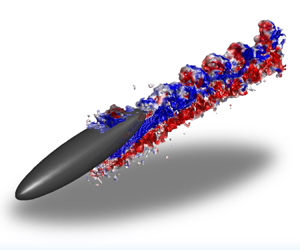
Figure 9(a,b) shows two views of the wake structure for  $\mathrm {R}5\mathrm {F}\infty \theta 10$. The streamwise vorticity field,
 $\omega _x(x, y, z)$, in figure 9(a) shows patches of negative streamwise vorticity interspersed with vertical protrusions of positive vorticity. The angled plane tilted in
 $y$ at
 $\theta _y=-10^\circ$ successfully tracks the higher amplitude fluctuations in
 $\omega _x$, which therefore lie parallel to the major axis of the spheroid. In figure 9(b), mushroom-like structures appear on the upper side of the wake.
(a) Streamwise vorticity,  $\omega _x (x, y, z)$, for R5F
 $\infty \theta 10$. The vertical plane
 $x0z$ slice is at
 $y/D=-0.25$ and the
 $x0y$ plane is inclined at
 $10^\circ$ starting at
 $z/D = -0.5$. The angled plane slice is an
 $x0y$ plane rotated about
 $y$ by
 $-10^\circ$ intersecting at
 $(x/D=0,y/D,z/D=-0.5)$. (b) Iso-surface of
 $Q$ (threshold
 $Q=0.56$), coloured by lateral vorticity
 $\omega _y$. A magnified view of a box is shown on the right. A transparent yellow plane at
 $x/D = 5.07$ corresponds to the slice location shown in panel (c). (c)
 $y0z$ slice of time-averaged streamwise vorticity
 $\overline {\omega _x}$ through a structure. The core radius
 $a$ and spacing
 $b$ are measured from the black contour line at
 $\overline {\omega _x}=0.607\omega _{x,\mathrm {max}}$.

The spacing,  $\lambda _s$, between these undulations along the streamwise vortices is of the order of the body diameter. They are not the same as the persistent coherent structures that last into the far wake, first measured at
 $x/D \geq 100$ (Meunier & Spedding Reference Meunier and Spedding2004); rather they are clearly visible for
 $3 \leq x/D \leq 6$. Colinear, counter-rotating vortices are subject to long- (Crow Reference Crow1970) and short-wavelength (Meunier & Leweke Reference Meunier and Leweke2005; Leweke et al. Reference Leweke, Le Dizès and Williamson2016) instabilities whose relative growth rates depend on the core size and spacing between vortices. Estimates of the core radius,
 $a$, and spacing,
 $b$, can be made from data such as shown in figure 9(c). The core is defined by a contour of
 $60.7\,\%$ of the maximum. Here,
 $2a$ is the minor axis diameter of the contour and
 $b/2$ is the distance from the centre of the core to the boundary of the vortex pair. For the unstratified wakes,
 $a \approx 0.12D$ and
 $b \approx 0.41D$ for
 $a/b \approx 0.29$. When
 $\lambda _s = 1.15D$, then
 $\lambda _s/a = 10$ and
 $\lambda _s/b = 2.8$. The most amplified scale in a Crow instability has
 $\lambda /b = 8.6$, while for the shorter wavelength elliptic instability,
 $\lambda /b = 0.4\unicode{x2013}1$, depending on Re.
The observed wavelengths ( $\lambda _s/b=2.8$) are split between the two most well-known alternatives. The generating conditions are not perfectly aligned, uniform colinear vortices, and their evolution is complicated by the presence of secondary vortices and the nearby drag wake and its turbulent fluctuations. The estimates above are for the unstratified case and details for the stratified ambient are not yet available, but a background density gradient is known to modify the instabilities on a vortex pair as shown in both laboratory and numerical experiments (Delisi & Robins Reference Delisi and Robins2000; Nomura et al. Reference Nomura, Tsutsui, Mahoney and Rottman2006).
3.2.2. Asymmetry in streamwise vortices
Figure 10(a) shows a sequence of slices in  $x/D$ where streamwise vortices are shed from the inclined body and develop downstream with increasingly evident asymmetry. The red patches of
 $\overline {\omega _x}$ show the counterclockwise rotating vortices (when viewed from positive
 $x$) are larger than their clockwise-rotating counterparts, which diminish in strength more rapidly. A second example is shown in figure 10(b) for R10F
 ${\infty \theta }20$, where the centroids are traced in the
 $y0z$ plane. The trajectories of the positive and negative vortices centre around the trajectory of the separation vortex pair observed by Jemison et al. (Reference Jemison, Delaney and Kannepalli2020), then they start to diverge at
 $x/D=6$, as also observed by Andersson, Jiang & Okulov (Reference Andersson, Jiang and Okulov2019). There is no preferred sign of the strongest circulation. A similar result was described by Ashok et al. (Reference Ashok, Van Buren and Smits2015), where pitching a DARPA SUBOFF model showed an initial asymmetry in strength (approximately
 $20\,\%$), which amplified downstream. In the yaw case, the weaker vortex was wrapped around and eventually annihilated by the stronger vortex. In the SUBOFF experiment and here, the symmetric state does not appear to be stable or reachable.
(a) Time-averaged streamwise vorticity  $\overline {\omega _x}$ for R5F
 $\infty \theta 10$ on
 $y0z$ slices at every
 $x/D=2$. (b) The trajectory of positive (red) and negative (blue) streamwise vorticity centroids for R10F
 ${\infty \theta 20}$. The dashed line is from Jemison, Delaney & Kannepalli (Reference Jemison, Delaney and Kannepalli2020)

Asymmetry becomes measurable aft of the body, and the configuration of this series of experiments is not focused on resolving details close to the body. Figure 11 shows details in the instantaneous  $u$,
 $v$ and
 $\omega _z$ fields from the intersection of a horizontal laser sheet with the body inclined at
 $20^\circ$ (R5F
 $\infty \theta 20$). The
 $u(x,y)$ signature is not exactly symmetric and there are shapes that resemble spiral motion superimposed on top of the two defect regions extending streamwise either side of the body. The spiral shapes are similar in size and amplitude but out of phase. The
 $v(x,y)$ field is consistent with an oblique cut through the streamwise vortices with the change in sign in
 $v$ coming as the interrogation sheet cuts through the core. The spatial gradients of the two fields combine to yield the vertical vorticity,
 $\omega _z$ in figure 11(c). The principal streamwise vortices leave no direct trace, but instead, the fine details of secondary flows are emphasised. These details are qualitatively consistent with the pattern of primary and secondary separation vortices previously noted (Fu et al. Reference Fu, Shekarriz, Katz and Huang1994; Xiao et al. Reference Xiao, Zhang, Huang, Chen and Fu2007).
(a)  $u/U$, (b)
 $v/U$ and (c)
 $\omega _z D/U$ on a horizontal
 $x0y$ plane for R5F
 $\infty \theta 20$. The dashed line shows the projected view of the inclined spheroid on the horizontal plane.

3.2.3. Wake propagation
The reduction in vertical extent of stratified wakes has already been demonstrated in the  $u(x, z)$ fields of figure 8. Figure 12 shows the time-averaged velocity field for all cases of
 $\theta = 20^\circ$ over as great a range of
 $x/D$ as available, and where the averaged field allows a systematic tracing of the wake defect. Three effects can be observed. At each Re–Fr pair, wake migration in the
 $z$-direction is inhibited, though the maximum height in
 $z$ increases as Fr increases. The unstratified wakes have greater extent in
 $z$ and are weaker than their stratified counterparts. Finally, when the stratified wakes reach their maximum height, they then contract slightly and undulate with a wavelength that increases with Fr. It is once again notable that stratification quite strongly influences the wake trajectory even when
 ${\textit {Fr}} = 64$.
 $\bar {u}(x, z)$ in a vertical centreplane for: (a) R5F
 $\infty$; (b) R5F16; (c) R10F
 $\infty$; (d) R10F32; (e) R20F
 $\infty$; ( f) R20F64. All are for
 $\theta = 20^\circ$. The blue dashed line traces
 $\bar {u}_0(x, z)$ and the purple line marks the wake edge where
 $\bar {u}(z) = 0.5 \bar {u}_0$.

The similar undulations that scale with Fr suggests a process that occurs in buoyancy time scales, and the wake centreline trajectories of all three stratified cases are shown in figure 13. The peak displacement occurs between  $Nt = 2$ and 3, with higher Fr maxima occurring slightly later in buoyancy times. With increasing Fr, there is an increase in both initial and maximum
 $z_0$. This offset is not the same as a wave amplitude, which can be estimated from the difference in
 $z_0$ from the first peak to the first minimum, and is plotted in figure 14 as a function of Fr, alongside the wavelength
 $\lambda$, estimated from the same data. There is no clear relationship between either
 $\lambda$ or
 $\zeta$ with Fr, in contrast to findings by Meunier et al. (Reference Meunier, Le Dizés, Redekopp and Spedding2018) where
 $\lambda$ increased linearly with increasing Fr and
 $\zeta$ decreased for both lee waves and wake-generated waves. Here, the forcing does not come from a resonance of the body diameter length scale with the ambient density gradient, nor does it arise from the wake-element dynamics associated with wake-generated waves. Rather it is a response of the stratified background to a vertical impulse caused by the passage of the inclined body, whose wake swirls around and adheres to the body length up until separation of the streamwise vortices. This separation point does not depend strongly on Fr, and the ambient fluid response at frequency
 $N$ is set by
 ${\partial \rho }/{\partial z}$.
Trajectory of wake centreline,  $\bar {u}_0$, scaled in
 $Nt$ of all stratified cases (R5F16, R10F32 and R20F64).

(a) The wavelength  $\lambda /D$ and (b) the amplitude
 $\zeta /D$ of the wake trajectory in figure 13 as a function of Fr. The size of the marker indicates the uncertainty of the measurement.

Re and Fr vary together, but in the unstratified cases of figures 8(a)–8(c), there is little obvious dependence of the wake geometry on Re. In figures 12(b), 12(d), 12( f), the vertical excursions extend in  $x/D$ as Fr increases. Since Fr is a measure of eddy turnover time scales to buoyancy time scales, more turnover times occur before some fixed
 $Nt$ at higher Fr (recall
 $x/D = Nt ({\textit {Fr}}/2)$).
When the body is inclined, the initial wake disturbance has a component that follows the shape of the body (the initial trajectory of the separated streamwise vortices also lies close to the body), and the wake imparts a vertical impulse to the density-stratified fluid. The response is a relaxation on time scales of  $1/N$, and in figure 15, there is a response in
 $\bar {w}(Nt)$ with a time scale of approximately
 $Nt = 2{\rm \pi}$. This time scale is independent of Fr over
 $16 \leq {\textit {Fr}} \leq 64$, and it is also independent of Re.
Averaged vertical velocity  $\bar {w}/U$ in
 $Nt$ of: (a) R5F16; (b) R10F32; and (c) R20F64.

3.2.4. Evolution of length and velocity scales for non-zero $\theta$

Inclined spheroids leave complex, hybrid wakes with an amalgam of signatures from the trailing streamwise vortices originally shed from some point along the body, together with the usual turbulent wake originating from the shear layers separating close to the lee. The wake is also inclined at some angle which decreases with  $x/D$, so transects at fixed streamwise location make varying oblique angles through the structure. Figure 16(a) shows a set of
 $\bar {u}_0(z)$ profiles at varying
 $x/D$ for R10F
 $\infty$ and R10F32. The time-averaged wake defect profiles initially (at
 $x/D = 10$) resemble a slightly asymmetric Gaussian, but the asymmetry grows more pronounced with
 $x/D$ for both unstratified and stratified wakes. The defect is stronger in
 $z < z_0$, which in this experiment is the region impacted by the streamwise vortices and their associated disturbance. Though
 $\omega _x$ conveys no signature upon
 $u$, the lifting off of the separated region will be linked with the shedding of low-speed fluid from the boundary layer. The last available profile in the unstratified data is at
 $x/D = 40$ because the wake leaves the observation window. The stratified profiles can be followed for longer and are shown in figure 16(b). Now the asymmetry decreases with increasing
 $Nt$, indicating that buoyancy acts to keep the wake components closer together in
 $z$. This is even accompanied by a return close to symmetry, as shown in figure 16(c). The time when symmetry is restored is at
 $Nt = 5{\rm \pi} /2$.
 $\bar {u}(z)$ centred at
 $z_0$ where
 $\bar {u} = u_0$. (a) R10,
 ${\textit {Fr}}=\{\infty,32\}$ at
 $x/D=\{10,20,40\}$ and (b) R10F32 at
 $Nt=\{1/4,1,5/2\}{\rm \pi}$. (c) Half-profile of
 $+z$ and reversed
 $-z$ of R10F32 at
 $Nt=5/2{\rm \pi}$. Red dotted lines in panels (a,b), and a black dotted line in panel (c) are Gaussian fit profiles.

Describing these curves with a single length and velocity scale does not include variations in profile shape as streamwise vortices combine with the turbulent drag wake, and figure 17(a) has a range of more than a factor of two in initial value before the curves coalesce over  $5 \leq x/D \leq 10$. After that, there is considerable variation in the vertical growth rates, though the unstratified wakes always grow faster. At the same time, the centreline velocity of the unstratified wakes always decays faster (figure 17b), starting at approximately
 $x/D = 10$. Plotting
 $L_V$ and
 $\bar {u}_0$ as a function of
 $Nt$ for the stratified cases, figure 17(c,d) shows signs of convergence of the data after
 $Nt \approx 2$, where
 $L_V$ increases only slowly and
 $\bar {u}_0$ also decays slowly. The data do not extend beyond
 $Nt = 10$, which would remain within the expected NEQ regime. At
 $Nt = 10$, the normalised
 $L_V \approx 0.5$ and normalised
 $\bar {u}_0 \approx 0.5$. The equivalent values for the
 $\theta = 0^\circ$ case are
 $L_V \approx 0.5$ and
 $\bar {u}_0 \approx 0.3$. The similarity of these data suggest that inclined spheroid wakes may not be statistically different from their uninclined equivalents by the end of the NEQ regime, so the long-time evolution may also then be similar.
(a,c) Vertical length scale,  $L_V$, and (b,d) centreline velocity,
 $\overline {u_0}/U$, for the inclined spheroid at
 $\theta = 20^\circ$. Panels (c,d) show rescaled measures based on predicted variations with
 $Nt$. Unstratified data shown with black lines and stratified with blue lines. The Re variation is shown as R5 (solid), R10 (dash), R20(dotted). Black and blue shading show the uncertainty for unstratified and stratified cases, respectively.

3.2.5. Lateral asymmetry
When the spheroid wake is examined as a distribution of  $\bar {u}(x, y, z)$, it appears as a mix of features originating from boundary layers that have separated at various points upstream. In other measures, however, the dominant signature comes from the streamwise vortices forming a counter-rotating pair (figure 18a). If the vortex pair were symmetric in strength and location,
 $\bar {v}(x, z)$ would have no coherent pattern in the vertical centreline. Instead, a band of positive and negative
 $\bar {v}$ appear at all Fr. These bands bend to follow the body and then reach a maximum height, which increases with Fr. This maximum height is reached by
 $Nt = 2$ in all cases. The figures shows that the shed vortices are not symmetric about the centreline, and the sign of asymmetry is the same each time. It is likely the sign of the symmetry breaking reflects an asymmetry in the geometry or kinematics of the experiment, though attempts to identify the source were not successful. Indeed, exact symmetry in this configuration appears to be a fragile and unrealisable state. The vertical migration of the vortex pair is restricted by the background stratification, which imposes a response in approximately constant
 $Nt$.
(a) Evolution of  $\bar {v}(z)$ versus
 $Nt$ for R5F16 (top), R10F32 (middle), R20F64 (bottom). The abscissa covers a fixed range in
 $Nt$, corresponding to larger
 $x/D$ as Fr increases (
 $Nt = (x/D) (2/{\textit {Fr}})$. (b)
 $\bar {v}(y, z)$ at increments of
 $x/D = 2$ for the unstratified case of R5F
 ${\infty \theta }10$.

The asymmetry is not restricted to stratified cases, and figure 18(b) shows cross-stream cuts through the wake of a body inclined at  $\theta = 10^\circ$ and no stratification. At
 $x/D = 0$ (which is defined here as the location halfway along the body,
 $L/2$),
 $\bar {v}$ is positive on the upper side of the body and negative on the lower side. Note how the body travels in
 $-x$, leaving a wake that extends in
 $+x$. The inclination angle,
 $\theta$, is defined positive for nose down so the wake data come from the side that has no, or little, interference with the support lines. The functional underside of the body is thus on the top and flow swirls around the body from (functional) bottom to top. Separated from the top surface, the lateral flow is towards the centreline (negative blue patches) and, closer to the body surface, there is a return (red) flow. These are the hydrodynamic footprints of the primary separation vortices, which loosely track the body angle so the whole wake is inclined upwards. The rotating motion around the body on either side generates a characteristic quadrangle pattern at
 $x/D = 4$ with alternating signs of
 $\bar {v}$ on either side, and the same sign on each diagonal. The asymmetry in strength and size of the vortex patches can be traced back to the first plane at
 $x = 0$. Thereafter, the wake continues to develop asymmetrically and the patches of
 $\bar {v}$ rotate around each other.
A simple cartoon showing the proposed interpretation of these data is given in figure 19, where the asymmetry in initial circulation of the streamwise vorticity is responsible for the observed patterns in figures 18(a) and 18(b). It further matches the cuts of  $\omega _x(y, z)$ in figure 10(b).
A sketch of counter-rotating vortex pair originating on one side of an inclined body, with unequal initial strengths and which then evolve downstream to yield distributions of  $\bar {v}$ and
 $\omega _x$, as observed in figures 18(a,b) and 10(b).

4. Summary and conclusions
For the (special) case of  $\theta = 0^\circ$, there is little change from previous studies on slender bodies. Though
 $St$ may increase slightly with background stratification in early wakes (
 $x/D \leq 10$), as also shown over
 $10 \leq x/D \leq 70$ in simulations by Ortiz-Tarin et al. (Reference Ortiz-Tarin, Nidhan and Sarkar2021, Reference Ortiz-Tarin, Nidhan and Sarkar2023), there is little evidence that this variation persists into the far wakes. Here,
 $x/D \geq 70$. A rescaled
 ${St}_m$ based on a momentum thickness,
 $D_m$, agrees with previous data from Meunier & Spedding (Reference Meunier and Spedding2004) by the time the far wake is encountered, and conditions entering this stage of wake evolution do not differ from the previous experimental data.
When compared with their unstratified equivalent, stratified wakes have a reduced vertical extent ( $L_V$) and a lower decay rate of centreline velocity,
 $u_0$. There are no obvious power laws for either quantity in the early wake, and no attempt has been made to identify transitions between regimes (e.g. 3-D-NEQ-Q2-D). The data do not clearly scale with stratification parameters in
 $Nt$, and there is considerable scatter between conditions in Re, Fr,
 $\theta$. There are some signs that similar wake properties are measurable by
 $x/D = 100$ or
 $Nt = 10$. By that distance/time, the differences between stratified and unstratified cases are clearly established, and the normalised
 $\bar {u}_0/U.{\textit {Fr}}^{2/3}$ has a value of approximately 0.4 at
 $Nt = 10$.
When the spheroid travels with its body tilted from the axis of travel, the flow around it separates before the end of the body to form streamwise vortices which mix with and modify the wake. The most notable net effect is that the wake initially propagates upwards at an angle slightly less than  $\theta$, and imparts a vertical impulse to the stable background stratification. The whole wake then relaxes back to an equilibrium position, about which it undulates with period
 $2{\rm \pi} /N$. At the same time, local measures of wake height (tracking the large-scale excursion)
 $(L_V/D){\textit {Fr}}^{-1/3} \approx 0.5$, and centreline velocity
 $(\bar {u}_0/U){\textit {Fr}}^{2/3} \approx 0.3$ are similar to those measured for the
 $\theta = 0^\circ$ case, suggesting similar dynamics within the wakes by
 $Nt = 10$.
The streamwise vortices themselves show evidence of secondary instabilities along their length, but the scale of these fluctuations does not match neatly with theoretical/empirical predictions, lying somewhere between the scales predicted for a Crow or elliptic instability. The somewhat inconclusive outcome is perhaps unsurprising because the environment is not otherwise free of inhomogeneities.
The streamwise vortices migrate vertically against the density gradient and then stop at a displacement that depends on Fr. They are not symmetric in initial strength/size and this disparity is retained further downstream. The lack of symmetry agrees with previous findings in unstratified, slender body wakes, from experiments on a SUBOFF model (Ashok et al. Reference Ashok, Van Buren and Smits2015) at high Re, and from simulations on a 6 : 1 spheroid at  $Re = 3000$ (Jiang et al. Reference Jiang, Gallardo, Andersson and Okulov2016). The latter simulations showed that the asymmetric wake was responsible for lateral forces that came up to 75 % of the streamwise force and that the asymmetry was more pronounced with increasing Re. We cannot rule out small asymmetries in experimental details here, but it appears the asymmetric state is a preferred, stable attractor.
In some respects, this study may be regarded as preliminary in the sense that although equivalent Re allows stratified and unstratified conditions to be directly compared, the stratified data are restricted to the track of maximum constant  $N$ allowed by the practical conditions of refractive index matching in the tow tank. Consequently, variations in
 $U$ cause proportional changes in both Re and Fr. The study has also focused solely on the vortex wakes, with no systematic attempt to investigate the role of internal gravity waves, either from the body or from the wake. The lowest
 $Fr = 16$ may seem high for significant body-induced lee waves, but
 ${\textit {Fr}}_L = 16/6$ is not so large. For
 $Fr = 32$ and 64, the wake itself is expected to become a more significant source of internal waves (Abdilghanie & Diamessis Reference Abdilghanie and Diamessis2013; Meunier et al. Reference Meunier, Le Dizés, Redekopp and Spedding2018; Zhou & Diamessis Reference Zhou and Diamessis2019), and horizontal interrogation planes or volumes offset from the wake centre will be informative on propagating wake components in these conditions.
Acknowledgements
The authors thank E. Singer and M. Oliver at the University of Southern California for their assistance in collecting experimental data.
Funding
This work was sponsored by the Office of Naval Research (ONR) Grant N0014-20-1-2584 under the management of Dr P. Chang.
Declaration of interests
The authors report no conflict of interest.


 Open access

