1. Introduction
In the microscale/nanoscale, the surface forces, for example surface tension force, and electrical force, are regarded as effective means to control both the fluid flow and particle motion. As the scale decreases, the body forces become negligible and the surface forces dominate the fluid flow. The electrical force is considered a typical surface force and it can significantly affect the flow behaviours through various phenomena including electrowetting, dielectrophoresis and electroosmosis (Liang et al. Reference Liang, Zhang, Li, Xia, Wu, Ge, Huang and Chou2005; Mugele & Baret Reference Mugele and Baret2005; Wheeler Reference Wheeler2008; Pethig Reference Pethig2010; Alizadeh et al. Reference Alizadeh, Hsu, Wang and Daiguji2021). The application of an electric field is an effective method for manipulating both conductive materials and dielectric ones. When an electric field is imposed on the dielectric materials, polarisation charges are induced at the interface and thus an electrical force is generated (Jackson Reference Jackson1999; Roberts & Kumar Reference Roberts and Kumar2009; Tsori Reference Tsori2009). The application of an electric field has been widely used in a variety of applications in microfluidic chips, including droplets generation and manipulation, tuneable microlens and particle separation (Pethig Reference Pethig2010; Li et al. Reference Li, Ding, Shao, Tian and Liu2012, Reference Li, Ha, Liu, Van Dam and Kim2019).
The non-uniform electrical force has also been used to fabricate micropatterns/nanopatterns, while the respective process is termed as electrohydrodynamic patterning (Chou, Zhuang & Guo Reference Chou, Zhuang and Guo1999; Schaffer et al. Reference Schaffer, Thurn-Albrecht, Russell and Steiner2000; Wu & Russel Reference Wu and Russel2009). A typical set-up of the electrohydrodynamic patterning is depicted in figure 1(a). A liquid–air or a liquid–liquid film is sandwiched between a topographical template and a flat substrate. After imposing the voltage, a non-uniform electrical force is generated along the liquid–air interface due to the modulation of the topographical template. The induced electrical force is stronger underneath the protrusion and weaker beneath the cavity. This non-uniform force drives fluid flow within the liquid film, leading to deformation. Electrohydrodynamic patterning can be considered a replication technique, as the deformation in the liquid film typically conforms to the template’s geometry (Wu & Russel Reference Wu and Russel2009). By adjusting the template topography, voltage and other parameters such as periodic pillars, stripes, triangles and concentric circles have been achieved (Mukherjee & Sharma Reference Mukherjee and Sharma2015). The deformed liquid film can also be solidified into micropatterns/nanopatterns for various applications (Hu et al. Reference Hu, Shao, Tian, Li and Jiang2016, Reference Hu, Tian, Shao, Li, Wang, Wang, Tian and Lu2017). A similar configuration is to use a flat plate as the top template which is usually termed as electrohydrodynamic instability or lithographically induced self-assembly (Chou & Zhuang Reference Chou and Zhuang1999). Although the electric force along the liquid film is uniform at the initial state, the system is unstable. Perturbations with certain wavelengths along the liquid film are amplified by the electric field, eventually leading to the formation of periodic micropatterns/nanopatterns (typically pillars) in liquid film. However, compared with the electrohydrodynamic patterning, the controllability of electrohydrodynamic instability is not satisfied. Therefore, electrohydrodynamic patterning is more frequently used in experiments for microfabrication/nanofabrication.
From a theoretical perspective, numerous studies have investigated the dynamic processes of electrohydrodynamic patterning through analytical and numerical simulations (Verma et al. Reference Verma, Sharma, Kargupta and Bhaumik2005; Wu, Pease & Russel Reference Wu, Pease and Russel2005; Wu & Russel Reference Wu and Russel2005; Kim & Lu Reference Kim and Lu2006; Gambhire & Thaokar Reference Gambhire and Thaokar2014). Electrohydrodynamic patterning is fundamentally a multiphysics problem, coupling the electric field with two-phase flow. To simplify the calculation, the long-wave approximation (i.e. lubrication approximation) is often employed (Pease & Russel Reference Pease and Russel2002). This approximation facilitates the solution of the electric field and reduces the fluid dynamics to classical thin-film flow. Based on the lubrication approximation, Wu & Chou (Reference Wu and Chou2003) developed a two-dimensional (2-D) mathematical model to study the dynamic process of electrohydrodynamic patterning. Wu et al. (Reference Wu, Pease and Russel2005) and Verma et al. (Reference Verma, Sharma, Kargupta and Bhaumik2005) extended this model to the three-dimensional (3-D) case and investigated the influence of template topography, film thickness and imposed voltage on the dynamic process. One similar case with the electrohydrodynamic patterning is the thin liquid film flows over the flat or topographic substrate (Blyth et al. Reference Blyth, Tseluiko, Lin and Kalliadasis2018). Tseluiko, Blyth & Papageorgiou (Reference Tseluiko, Blyth and Papageorgiou2013) studied the stability of film flow over inclined topography using a long-wave nonlinear model. They also explored the electrified film flow on inclined topographic substrate, assuming a uniform electric field (Tseluiko & Papageorgiou Reference Tseluiko and Papageorgiou2006; Tseluiko et al. Reference Tseluiko, Blyth, Papageorgiou and Vanden-Broeck2008a ,Reference Tseluiko, Blyth, Papageorgiou and Vanden-Broeck b ).
With the advances in computing technology, the implementation of fully nonlinear numerical models for electrohydrodynamic patterning has been proposed in the literature (Kim & Lu Reference Kim and Lu2006; Tian et al. Reference Tian, Shao, Ding, Li and Li2011; Yang et al. Reference Yang, Li and Ding2013a,Reference Yang, Li and Dingb ). These models are generally classified into two categories: moving-mesh methods and fixed-mesh methods. In moving-mesh methods, the traditional sharp interface is adopted. The two-phase flow is solved simultaneously with the associated boundary conditions at the fluid–fluid interface (Song et al. Reference Song, Liu, Zhang, Fan and Yang2022). Meanwhile, the computational domain is remeshed with the deformation of the free surface. In contrast, fixed-mesh methods such as the phase field method, the level set method, the front tracking method and the volume of fluid method treat the interface as a thin diffusive layer (Yang et al. Reference Yang, Li and Ding2013a , Reference Yang, Li, Shao and Ding2014). These methods typically introduce an extra parameter to distinguish the two different fluids. Compared with the moving-mesh methods, the advantage of fixed-mesh methods is that they are remeshing-free during the deformation free surface deformation. However, this benefit comes at the cost of increased computational complexity, as an additional equation must be solved, significantly increasing computing time, especially in 3-D cases.
While some studies have examined the dynamic process of electrohydrodynamic patterning, relatively little attention has been given to the equilibrium deformation. Yeoh, Xu & Basaran (Reference Yeoh, Xu and Basaran2007) proposed a numerical model based on the finite element method and studied the equilibrium deformation of electrohydrodynamic patterning. In their model, the top template was flat and grounded, while the electric potential of the bottom plate took a sinusoidal function. They found that the equilibrium deformation can be obtained if the imposed voltage is below a critical value. Heier, Groenewold & Steiner (Reference Heier, Groenewold and Steiner2009) experimentally observed equilibrium deformation, identifying two possible scenarios: either a slight deformation of the liquid film or a significant deformation leading to contact with the top template. Ramkrishnan & Kumar (Reference Ramkrishnan and Kumar2014) studied the dynamic process and also the equilibrium deformation of electrostatic assist gravure printing. Although their configuration differs from electrohydrodynamic patterning, the underlying mechanism remains the same. However, several fundamental aspects of electrohydrodynamic patterning remain unclear. (i) How to derive an explicit equation (analytical solution) for the equilibrium deformation of liquid film and the critical voltage? (ii) What is the equilibrium deformation under a high voltage (higher than the critical value)? (iii) For a given voltage, is there one unique equilibrium state or multiple equilibrium states? (iv) How to develop the mathematical model for the 3-D case? These questions constitute the central focus of this study.
In this work, two theoretical models are developed including the linear model and the nonlinear one to examine equilibrium deformation. It is found that the equilibrium deformation of the liquid film is closely dependent on the electric Bond number Bo E , the non-dimensional parameter representing the strength of the electric field. With the increase of Bo E , the deformation is also increased accordingly. When a critical value is achieved for Bo E , the deformation becomes remarkable and the film gets in direct contact with the upper template. Modelling this ‘contact’ scenario presents a challenge (Yeoh et al. Reference Yeoh, Xu and Basaran2007). Imposing a high voltage would lead to numerical divergence or physically unrealistic scenarios, such as film penetration of the upper template. To address this issue, a disjoining pressure between the liquid film and the template/substrate is incorporated into the model. The disjoining pressure has been adopted in other works when modelling the film flow (Wu et al. Reference Wu, Pease and Russel2005; Wu & Russel Reference Wu and Russel2006; Nazaripoor et al. Reference Nazaripoor, Koch, Sadrzadeh and Bhattacharjee2016, Reference Nazaripoor, Flynn, Koch and Sadrzadeh2018). Physically, the disjoining pressure indicates there are two repulsive forces, one is between the liquid film and the upper template, and the other is between the film and the substrate. This prevents film penetration and ensures a physically realistic outcome. With the consideration of disjoining pressure, the nonlinear model reveals the manifestation of more intriguing phenomena. For a given Bo E value, multiple (three at most) equilibrium states can take place. To analyse the stability, a function is defined to characterise the free energy. According to the free energy analysis results, among these three equilibrium states, one is stable, the other is metastable and the third one is unstable. At the end, the models are extended to the 3-D case.
Schematic illustration of the electrohydrodynamic patterning: (a) diagram of the designed configuration; (b) the computational domain.

2. Problem statement
As illustrated in figure 1(a), the liquid–air film is confined between a topographical template and a flat substrate. Without losing generality, a rectangular template is considered, as it is the most commonly used in experiments (Schaffer et al. Reference Schaffer, Thurn-Albrecht, Russell and Steiner2000; Wu & Russel Reference Wu and Russel2009). An external electric field with potential V
0 is imposed to the system. Due to the modulation of the template, a non-uniform electrical force is generated along the liquid–air interface. This force drives fluid flow within the liquid film, leading to its deformation. Both the liquid and air are assumed to be perfect dielectric materials, as the liquid in most cases is a monomer with low conductivity. The density and dielectric constants of air and liquid are denoted as
 $\rho$
a
(
 $\rho$
) and
 $\varepsilon $
1 (
 $\varepsilon $
2), respectively. The viscosity of air (liquid) is represented by
 $\mu $
a
(
 $\mu $
) (Cengel Reference Cengel2010). The distance between template and substrate is denoted by d
0, the initial thickness of the liquid film is h
0 and the structure height and width of the template are
 $\Delta$
d and w, respectively. We assume that the system is periodic, with a period λ. The liquid–air interface is represented as h(x), and the geometry of the template is d(x). The normal vector of the interface h(x), denoted by
 $\boldsymbol{n}$
, is pointing from liquid to air. For simplification, only one periodic structure is considered as the computational domain (figure 1
b).
3. Governing equations
3.1. Electric field
As was mentioned above, both liquid and air are treated as dielectric materials. The governing equation for the electric field is simplified to the Laplace equation (Jackson Reference Jackson1999),
 \begin{equation} \nabla ^{2}V_{i}=0 ,\end{equation}
where V
i
(
 $i=1$
, 2) stands for the electric potential in the air and liquid phase. Both air and liquid are considered as dielectric materials. The boundary conditions are listed as follows, V
2 = 0 at y = 0; V
1 = V
0 at y = d; V
1 = V
2 and
 $\varepsilon _{1}(({\partial V_{1}})/({\partial n})=\varepsilon _{2}(({\partial V_{2}})/({\partial n}))$
at y = h, where h denotes the liquid–air interface and d is the interface of template.
Prior to deriving the electric field in the electrohydrodynamic patterning, a scale analysis is performed. Some characteristic (reference) scaling parameters are introduced, with the characteristic lengths in the x and y directions chosen as λ and h
0, respectively, i.e. x
c
∼ λ, y
c
∼ h
0. The characteristic electric voltage is V
0. The governing equation (3.1), can be rewritten as
 ${({h_{0}}^{2})}/{(\lambda ^{2})}{(\partial ^{2}{V_{i}}^{*})}/{(\partial x^{*2})} + {(\partial ^{2}{V_{i}}^{*})}/{(\partial y^{*2})}=0$
, where superscript & denotes the non-dimensional parameter. In this paper, we focus on the case of thin liquid film, where the thickness of film is much smaller than the periodic length, h
0 << λ, or equivalently, h
0/λ < <1. With such an approximation, known as the lubrication approximation, the governing equation of electric field becomes
 ${(\partial ^{2}V_{i})}/{(\partial y^{2}})=0$
. Considering boundary conditions, one has the expressions of
 $V_{1}$
and
 $V_{2}$
,
 \begin{equation} \left\{\begin{array}{l} V_{1}=V_{0}-\dfrac{\varepsilon _{r}V_{0}\left(d-y\right)}{\varepsilon _{r}d-\left(\varepsilon _{r}-1\right)h}\\[9pt] V_{2}=\dfrac{V_{0}y}{\varepsilon _{r}d-\left(\varepsilon _{r}-1\right)h} \end{array}\right. \!.\end{equation}
The electric field strength in the vertical direction can be approximately expressed as (Rohlfs et al. Reference Rohlfs, Cammiade, Rietz and Scheid2021),
 \begin{equation} \left\{\begin{array}{l} E_{1}=-\dfrac{\partial V_{1}}{\partial y}=\dfrac{\varepsilon _{r}V_{0}}{\varepsilon _{r}d-\left(\varepsilon _{r}-1\right)h},\\[9pt] E_{2}=-\dfrac{\partial V_{2}}{\partial y}=\dfrac{V_{0}}{\varepsilon _{r}d-\left(\varepsilon _{r}-1\right)h}, \end{array}\right. \end{equation}
where E 1 and E 2 denote the electric field strength in air and liquid. As for the electric field in the x direction, it is approximately zero. The electric field is normal to the liquid–air interface. Due to the modulation of the template, the electric field along the liquid–air interface is non-uniform.
3.2. Flow field
The deformation of liquid–air interface is essentially caused by the flow field in the film. In this section, we derive the solution of fluid flow. The fluid flow in the film is governed by the Navier–Stokes equations (Kundu & Cohen Reference Kundu and Cohen2008),
 \begin{equation} \left\{\begin{array}{l} \rho \dfrac{\partial u}{\partial t} + \rho u\dfrac{\partial u}{\partial x} + \rho v\dfrac{\partial u}{\partial y}=-\dfrac{\partial p}{\partial x} + \mu \dfrac{\partial ^{2}u}{\partial x^{2}} + \mu \dfrac{\partial ^{2}u}{\partial y^{2}}\\[12pt] \rho \dfrac{\partial v}{\partial t} + \rho u\dfrac{\partial v}{\partial x} + \rho v\dfrac{\partial v}{\partial y}=-\dfrac{\partial p}{\partial y} + \mu \dfrac{\partial ^{2}v}{\partial x^{2}} + \mu \dfrac{\partial ^{2}v}{\partial y^{2}} \end{array}\right., \end{equation}
where u and v denote the velocity in the x and y directions,
 $\rho$
and
 $\mu $
stand for the density and viscosity of liquid (figure 1), p is the pressure in liquid. Gravity is insignificant in microflows/nanoflows and is thus ignored in this study. Moreover, the liquid is considered as an incompressible material. The mass conservation equation is expressed as
 \begin{equation} \frac{\partial u}{\partial x} + \frac{\partial v}{\partial y}=0. \end{equation}
Since these equations are difficult to solve analytically, some simplifications are made in this work. Characteristic velocities in the x and y directions are denoted by u 0 and v 0, respectively, i.e. u c ∼ u 0, v c ∼ v 0, where the subscript c denotes characteristic parameters. The characteristic length scales remain the same as in the electric field, i.e. x c ∼ λ, y c ∼ h 0. Substituting into (3.5), one obtains
 \begin{equation} \frac{u_{0}}{\lambda }\frac{\partial u^{\mathrm{*}}}{\partial x^{\mathrm{*}}} + \frac{v_{0}}{h_{0}}\frac{\partial v^{*}}{\partial y^{*}}=0. \end{equation}
In the above equation, the two terms have the same scale, thus
 $v_{0}\sim u_{0}h_{0}/\lambda$
. The characteristic time is chosen as
 $t_c \approx x_c/u_c=\lambda/u_0 $
. The characteristic pressure is chosen as
 $p_{c}\sim \mu u_{0}\lambda /{h_{0}}^{2}$
. Using these scaling parameters, (3.4) can be rewritten as follows:
 \begin{equation} \left\{\begin{array}{l} \mathrm{Re}\dfrac{{h_{0}}^{2}}{\lambda ^{2}}\dfrac{\partial u^{*}}{\partial t^{*}} + \mathrm{Re}\dfrac{{h_{0}}^{2}}{\lambda ^{2}}u^{*}\dfrac{\partial u^{*}}{\partial x^{*}} + \mathrm{Re}\dfrac{{h_{0}}^{2}}{\lambda ^{2}}v^{*}\dfrac{\partial u^{*}}{\partial y^{*}}=-\dfrac{\partial p^{\mathrm{*}}}{\partial x^{\mathrm{*}}} + \dfrac{{h_{0}}^{2}}{\lambda ^{2}}\dfrac{\partial ^{2}u^{*}}{\partial x^{*2}} + \dfrac{\partial ^{2}u}{\partial y^{2}}\\[12pt] \mathrm{Re}\dfrac{{h_{0}}^{4}}{\lambda ^{4}}\dfrac{\partial v^{\mathrm{*}}}{\partial t^{\mathrm{*}}} + \mathrm{Re}\dfrac{{h_{0}}^{4}}{\lambda ^{4}}u^{*}\dfrac{\partial v^{\mathrm{*}}}{\partial x^{\mathrm{*}}} + \mathrm{Re}\dfrac{{h_{0}}^{4}}{\lambda ^{4}}v^{\mathrm{*}}\dfrac{\partial v^{\mathrm{*}}}{\partial y^{\mathrm{*}}}=-\dfrac{\partial p^{\mathrm{*}}}{\partial y^{\mathrm{*}}} + \dfrac{{h_{0}}^{4}}{\lambda ^{4}}\dfrac{\partial ^{2}v^{\mathrm{*}}}{\partial x^{\mathrm{*}2}} + \dfrac{{h_{0}}^{2}}{\lambda ^{2}}\dfrac{\partial ^{2}v^{\mathrm{*}}}{\partial y^{\mathrm{*}2}} \end{array}\right. \!, \end{equation}
where
 $\mathrm{Re}=\rho u_{0}\lambda /\mu$
is the Reynolds number. If we neglect all the infinitesimal values and rewrite the equations in dimensional form, the Navier–Stokes equations reduce to
 \begin{equation} \left\{\begin{array}{l} 0=-\dfrac{\partial p}{\partial x} + \mu \dfrac{\partial ^{2}u}{\partial y^{2}}\\[9pt] 0=-\dfrac{\partial p}{\partial y} \end{array}\right. \!.\end{equation}
The flow is a pressure-driven Stokes flow, and the pressure p is constant in the y direction. In the x direction, the pressure gradient is balanced by the viscous force. To solve the velocity u, we can integrate (3.8a ) twice. However, the boundary conditions are still required.
At the liquid–air interface y = h, the force is balanced,
 \begin{equation} {\sigma _{ij}}^{\left(1\right)}\boldsymbol{\cdot} \boldsymbol{n}-{\sigma _{ij}}^{\left(2\right)}\boldsymbol{\cdot} \boldsymbol{n}=\gamma \boldsymbol{n}\nabla \boldsymbol{\cdot} \boldsymbol{n}-\nabla _{s}\gamma , \end{equation}
where
 ${\sigma _{ij}}^{(1)}$
and
 ${\sigma _{ij}}^{(2)}$
denote the stress tensor of air and liquid, respectively,
 $\boldsymbol{n}$
is the normal vector of the liquid–air interface, γ is the surface tension coefficient,
 $\nabla _{s}(\boldsymbol{\cdot} )=(I-\boldsymbol{n}\otimes \boldsymbol{n})\boldsymbol{\cdot} \nabla (\boldsymbol{\cdot} )$
,
I
is the identity matrix. In this study, the surface tension coefficient is considered to be constant, i.e.
 $\nabla _{s}\gamma =0$
. The stress tensors can be expressed as follows:
 \begin{equation} \left\{\begin{array}{l} {\sigma _{ij}}^{\left(1\right)}=-p_{0}I + \mu _{a}\left(\nabla \boldsymbol{u}_{a} + \nabla {\boldsymbol{u}_{a}}^{T}\right) + \varepsilon _{0}\varepsilon _{1}\left[\boldsymbol{E}_{1}\otimes \boldsymbol{E}_{1}-\dfrac{1}{2}\left(\boldsymbol{E}_{1}\boldsymbol{\cdot} \boldsymbol{E}_{1}\right)I\right]\\[9pt] {\sigma _{ij}}^{\left(2\right)}=-pI + \mu \left(\nabla \boldsymbol{u} + \nabla \boldsymbol{u}^{T}\right) + \varepsilon _{0}\varepsilon _{2}\left[\boldsymbol{E}_{2}\otimes \boldsymbol{E}_{2}-\dfrac{1}{2}\left(\boldsymbol{E}_{2}\boldsymbol{\cdot} \boldsymbol{E}_{2}\right)I\right] \end{array}\right. ,\end{equation}
where p
0 and p denote the pressure in air and liquid, respectively,
 $\boldsymbol{u}_{a}$
and
 $\boldsymbol{u}$
represent the velocity in air and liquid, respectively. As one can see, each stress tensor has three components. The first term originates from the hydrostatic pressure, the second term is from the viscous effect and the third one is the Maxwell stress tensor. The viscosity of air is much smaller than that of liquid and thus can be ignored,
 $\mu $
a
≈ 0. According to (3.3), the horizontal (x) component of electric field is zero.
In this study, the deformation on the liquid–air interface is assumed small,
 $({\partial h})/({\partial x})\ll 1$
. With this approximation, the convergence of the normal vector, i.e. the curvature, takes the form
 \begin{equation} \nabla \boldsymbol{\cdot} \boldsymbol{n}=-\frac{\partial ^{2}h}{\partial x^{2}}\left[1 + \left(\frac{\partial h}{\partial x}\right)^{2}\right]^{-\frac{3}{2}}\approx -\frac{\partial ^{2}h}{\partial x^{2}}. \end{equation}
Substituting, (3.9) can be written as follows:
 \begin{equation} \left\{\begin{array}{l} \left[p-p_{0}-2\mu \dfrac{\partial u}{\partial x} + \dfrac{1}{2}\varepsilon _{0}\left(\varepsilon _{2}{E_{2}}^{2}-\varepsilon _{1}{E_{1}}^{2}\right)\right]\dfrac{\partial h}{\partial x} + \mu \left(\dfrac{\partial u}{\partial y} + \dfrac{\partial v}{\partial x}\right)=\gamma \dfrac{\partial h}{\partial x}\dfrac{\partial ^{2}h}{\partial x^{2}}\\[9pt] \mu \left(\dfrac{\partial u}{\partial y} + \dfrac{\partial v}{\partial x}\right)\dfrac{\partial h}{\partial x} + p-p_{0}-2\mu \dfrac{\partial v}{\partial y}-\dfrac{1}{2}\varepsilon _{0}\left(\varepsilon _{2}{E_{2}}^{2}-\varepsilon _{1}{E_{1}}^{2}\right)=-\gamma \dfrac{\partial ^{2}h}{\partial x^{2}} \end{array}\right. \!. \end{equation}
According to the scale analysis, x
c
∼ λ, y
c
∼ h
0, h
c
∼ h
0, u
c
∼ u
0,
 $v_{c}\sim u_{0}h_{0}/\lambda$
and
 $p_{c}\sim \mu u_{0}\lambda /{h_{0}}^{2}$
. Therefore, one has
 ${\partial v}/{\partial x}\ll {\partial u}/{\partial y} , \mu {\partial v}/{\partial y}\ll p$
, and
 ${\partial h}/{\partial x}\ll 1$
. When infinitesimal terms are ignored, (3.2) reduce to
 \begin{equation} \left\{\begin{array}{l} \mu \dfrac{\partial u}{\partial y}\approx 0\\[5pt] p\approx p_{0} + \dfrac{1}{2}\varepsilon _{0}\left(\varepsilon _{2}{E_{2}}^{2}-\varepsilon _{1}{E_{1}}^{2}\right)-\gamma \dfrac{\partial ^{2}h}{\partial x^{2}} \end{array}\right. \!. \end{equation}
Equations (3.13) can be considered as the boundary conditions at y = h. At the bottom plate, no-slip condition is applied, so that the summarised boundary conditions for velocity are as follows:
 \begin{align} \left\{\begin{array}{lll} u=0 & at & y=0 \\ \mu \dfrac{\partial u}{\partial y}=0 & at & y=h \end{array}.\right. \end{align}
By integrating (3.8a ) twice with the boundary conditions (3.14), one gets the expression for velocity in liquid film (Wu & Chou Reference Wu and Chou2003; Nazaripoor et al. Reference Nazaripoor, Koch and Sadrzadeh2015, Reference Nazaripoor, Koch and Sadrzadeh2017),
 \begin{equation} u=\frac{1}{2\mu }\frac{\partial p}{\partial x}y^{2}-\frac{1}{\mu }\frac{\partial p}{\partial x}hy ,\end{equation}
where
 $\mu $
denotes the viscosity of the liquid, p represents the pressure.
According to (3.13b
), the pressure in the liquid consists of three components, the pressure of air p
0 which can be treated as constant, the electrostatic pressure
 $p_{e}=\varepsilon _{0}(\varepsilon _{2}{E_{2}}^{2}-\varepsilon _{1}{E_{1}}^{2})/2$
and the Laplace pressure caused by the surface tension
 $p_{\gamma }=-\gamma \nabla ^{2}h$
. Substituting (3.3) into (3.13b
), one has
 \begin{equation} p=p_{0}-\frac{1}{2}\frac{\varepsilon _{0}\varepsilon _{r}\left(\varepsilon _{2}-\varepsilon _{1}\right){V_{0}}^{2}}{\left[\varepsilon _{r}d-\left(\varepsilon _{r}-1\right)h\right]^{2}}-\gamma \frac{\partial ^{2}h}{\partial x^{2}}. \end{equation}
With the small deformation approximation, d ≈ d 0 and h ≈ h 0, the differentiation of pressure gives
 \begin{equation} \frac{\partial p}{\partial x}\approx -\frac{\varepsilon _{0}\varepsilon _{1}\varepsilon _{r}\left(\varepsilon _{r}-1\right){V_{0}}^{2}}{\left[\varepsilon _{r}\left(d_{0}-h_{0}\right) + h_{0}\right]^{3}}\left[\left(\varepsilon _{r}-1\right)\frac{\partial h}{\partial x}-\varepsilon _{r}\frac{\partial d}{\partial x}\right]-\gamma \frac{\partial ^{3}h}{\partial x^{3}}. \end{equation}
Substituting into (3.15), one gets the formula for velocity:
 \begin{equation} u=\frac{1}{2\mu }y\left(y-2h\right)\left\{-\frac{\varepsilon _{0}\varepsilon _{1}\varepsilon _{r}\left(\varepsilon _{r}-1\right){V_{0}}^{2}}{\left[\varepsilon _{r}\left(d_{0}-h_{0}\right) + h_{0}\right]^{3}}\left[\left(\varepsilon _{r}-1\right)\frac{\partial h}{\partial x}-\varepsilon _{r}\frac{\partial d}{\partial x}\right]-\gamma \frac{\partial ^{3}h}{\partial x^{3}}\right\}. \end{equation}
3.3. Interfacial evolution
The evolution of the interface is determined by the conservation of mass and can be expressed by the following equation:
 \begin{equation} \frac{\partial h}{\partial t}=-\frac{\partial }{\partial x}\left(\int _{0}^{h}u{\rm d}y\right). \end{equation}
Substituting the expression of velocity (3.16) gives the evolution of the liquid–air interface expressed as
 \begin{equation} \frac{\partial h}{\partial t} + \frac{\partial }{\partial x}\left\{\frac{\gamma h^{3}}{3\mu }\frac{\partial ^{3}h}{\partial x^{3}} + \frac{h^{3}\varepsilon _{0}\varepsilon _{1}\varepsilon _{r}\left(\varepsilon _{r}-1\right){V_{0}}^{2}}{3\mu \left[\varepsilon _{r}\left(d_{0}-h_{0}\right) + h_{0}\right]^{3}}\left[\left(\varepsilon _{r}-1\right)\frac{\partial h}{\partial x}-\varepsilon _{r}\frac{\partial d}{\partial x}\right]\right\}=0 .\end{equation}
To facilitate the analysis and discussion, the equation is normalised as follows:
 \begin{equation} \frac{\partial H}{\partial \tau } + \frac{\partial }{\partial X}\left\{\frac{1}{3}Ca^{-1}H^{3}\frac{\partial ^{3}H}{\partial X^{3}} + \frac{1}{3}Ca^{-1}Bo_{E}H^{3}\left[\left(\varepsilon _{r}-1\right)\frac{\partial H}{\partial X}-\varepsilon _{r}\frac{\partial D}{\partial X}\right]\right\}=0 \end{equation}
where τ = u
c
t/λ is the normalised time, u
c
= h
0
γ/λμ denotes the characteristic velocity, H = h/h
0 represents the normalised film thickness, D = d/h
0 is the normalised template–substrate distance and X = x/λ refers to the normalised length. After normalisation, the computational domain becomes [0, 1]. Additionally, the Capillary number is defined as
 $Ca=\mu u_{c}\lambda ^{3}/\gamma {h_{0}}^{3}$
, and the electric Bond number can be expressed as
 $Bo_{E}=\varepsilon _{0}\varepsilon _{1}\varepsilon _{r}(\varepsilon _{r}-1)\lambda ^{2}{V_{0}}^{2}/\gamma [\varepsilon _{r}(d_{0}-h_{0}) + h_{0}]^{3}$
.
The interest of this work is the equilibrium deformation (i.e. steady state) of the liquid film. At equilibrium, the interface ceases to evolve, i.e.
 $\partial H/\partial \tau =0$
. Then, (3.21) becomes
 \begin{equation} \frac{\partial ^{3}H}{\partial X^{3}} + Bo_{E}\left[\left(\varepsilon _{r}-1\right)\frac{\partial H}{\partial X}-\varepsilon _{r}\frac{\partial D}{\partial X}\right]=\frac{C}{H^{3}} \end{equation}
where C is a constant. Integrating (3.22) in the domain [0, 1] we get
 \begin{equation} \int _{0}^{1}\frac{\partial ^{3}H}{\partial X^{3}}{\rm d}X + \int _{0}^{1}Bo_{E}\left[\left(\varepsilon _{r}-1\right)\frac{\partial H}{\partial X}-\varepsilon _{r}\frac{\partial D}{\partial X}\right]{\rm d}X=\int _{0}^{1}\frac{C}{H^{3}}{\rm d}X .\end{equation}
Since H(X) and D(X) are periodic functions with the periodic length 1, the two terms on the left-hand side in (3.23) vanish due to periodicity. This implies that the right-hand side must also vanish, leading to C = 0. Essentially, the constant C is from the integral of velocity, which is the term in the parentheses in (3.19). Therefore, C can be considered as the non-dimensional flow rate. From (3.22), it follows that the viscosity
 $\mu $
does not influence the equilibrium deformation of electrohydrodynamic patterning.
4. Linear model
A linear model is proposed to study the equilibrium deformation of electrohydrodynamic patterning, where ‘linear’ refers to the geometry of the template D(X) and the liquid–air interface H(X). Both D(X) and H(X) are decomposed into Fourier series, retaining only the zeroth and first-order terms while truncating higher-order terms,
 \begin{equation} \left\{\begin{array}{l} D(X)\approx D_{0} + \dfrac{2}{\pi }\Delta D\cos \left(2\pi X\right)\\[5pt] H(X)\approx 1-H_{1}\cos \left(2\pi X\right) \end{array}\right. \end{equation}
where ΔD is the structure height of the template, and H 1 denotes the deformation amplitude of the liquid film. It is worth mentioning that the structure width of template is half of the periodic length λ/2. In this work, the structure height ΔH is chosen to quantify the deformation of the liquid film, which is defined as the difference between the highest point and the lowest one. In the linear model, it is assumed that ΔH = 2H 1. By substituting D(X) and H(X) into (3.22), the structure height can be obtained as follows:
 \begin{equation} \Delta H=\frac{4\varepsilon _{r}\Delta D}{4\pi ^{3}B{o_{E}}^{-1}-\pi \left(\varepsilon _{r}-1\right)}. \end{equation}
The structure height ΔH strongly depends on the following parameters, such as the electrical permittivity ratio
 $\varepsilon $
r
, the structure height of the template ΔD, and the electric Bond number Bo
E
.
A set of default parameters values are defined, which are the following: h
0 = 50 nm, d
0 = 125 nm, Δd = 50 nm, λ = 400 nm, w = 200 nm, γ = 28.9 mN m–1,
 $\mu $
= 300 Pa·s,
 $\varepsilon $
1 = 1,
 $\varepsilon $
2 = 5.24, V
0 = 36.7 V, where the physical parameters correspond to the polymethyl methacrylate material (Lin et al. Reference Lin, Kerle, Russell, Schäffer and Steiner2002). The corresponding non-dimensional parameters are, D
0 = 2.5, ΔD = 1,
 $\varepsilon $
r
= 5.24 and Bo
E
= 16.9. These parameters are used in the following sections unless explicitly indicated. Substituting them into (4.2), the liquid film deformation is obtained. Figure 2(a) illustrates the dependence of the structure height ΔH on the electric Bond number Bo
E
. The dashed blue line represents the solutions of (4.2), which are mathematically possible but physically impossible. When
 $\varepsilon $
r
> 1, the value of Bo
E
is positive, and thus only the solid line in figure 2(a) exists in experiments. As shown, ΔH increases monotonically with Bo
E
. At equilibrium, the electrostatic pressure is compensated by the surface tension pressure. A large Bo
E
value corresponds to a high voltage and electrostatic pressure, resulting in the development of a large deformation in the liquid film.
The deformation of the electrohydrodynamic patterning by the linear model. (a) The relationship between the equilibrium structure height
 $\Delta$
H and the electric bond number Bo
E
, when
 $\varepsilon $
r
= 5.24, (b)
 $\varepsilon $
r
= 0.19. (c) The velocity in the liquid film for non-equilibrium deformation and equilibrium deformation with
 $\varepsilon $
r
= 5.24. The colour bar represents the magnitude of normalised velocity. Here A-A denotes the transverse line where the velocity profile is displayed.

Another phenomenon can be ascertained in figure 2(a), where a critical value Bo
E,c
exists. When the electric Bond number approaches this value, the structure height
 $\Delta$
H asymptotically approaches infinity. Analyzing (4.2) reveals that
 $\Delta$
H goes to infinity when the denominator approaches zero. The corresponding electric Bond number is given by
 \begin{equation} Bo_{E,c}=\frac{4\pi ^{2}}{\varepsilon _{r}-1}. \end{equation}
This value is defined as the critical electric Bond number Bo E,c . To obtain micro patterns/nanopatterns with significant deformation, the applied Bo E must exceed this critical value. Usually, the microstructures with large deformation are of interest to experimentalists, yet it is challenging to achieve them with traditional methods (e.g. lithography, nanoimprint). Thus, the researchers are seeking novel fabrication methods for largely deformed microstructures, and the electrohydrodynamic patterning is considered as one promising candidate.
For the electrohydrodynamic patterning, the electrical permittivity ratio
 $\varepsilon $
r
is regarded as a key parameter. A particular case is
 $\varepsilon $
r
= 1, when the upper and the bottom layers have the same electrical permittivity. The electrical force along the interface vanishes in this case, and the electrohydrodynamic patterning does not occur. Typically, in experiments the bottom layer (liquid) has a larger electrical permittivity than the upper layer (air), i.e.
 $\varepsilon $
r
> 1. In such case, the electric Bond number Bo
E
> 0, producing a structure in the liquid film which is a positive replica of the template (figure 2
a). In the opposite case, when
 $\varepsilon $
r
< 1, the corresponding electric Bond number is negative Bo
E
< 0. This situation corresponds to the case that the liquid and the air interchange their positions, namely, the liquid layer is on the top and the air is beneath. In this circumstance, the obtained structure is a negative replica of the template. Figure 2(b) illustrates the relationship of the ΔH and Bo
E
parameters when the electric Bond number is chosen as
 $\varepsilon $
r
= 0.19. The negative ΔH indicates that the structure in the liquid film has a phase difference π with the template. When the electric Bond number approaches the critical value of Bo
E,c
= 4π2/(
 $\varepsilon $
r
− 1), the structure height approaches the negative infinity.
With the given parameters and deformation H(X), the flow field can be determined from (3.22). When the liquid film is flat, ΔH = 0, the velocity profile follows a parabolic shape (figure 2 c), where the velocity has been normalised by the characteristic velocity of u c = h 0 γ/λμ. When the equilibrium state is achieved, ΔH = 1.3, the velocity becomes zero. At the equilibrium state, the generated electrostatic pressure is completely balanced by the surface tension pressure. Thus, the hydrostatic pressure p becomes uniform and the fluid flow vanishes.
5. Nonlinear model
The primary advantage of linear model is its simplicity, enabling an explicit calculation of deformation. However, truncating higher-order terms sacrifices accuracy. According to the linear model, the structure height
 $\Delta$
H approaches the infinity when Bo
E
approaches the critical value. However, an infinite
 $\Delta$
H value is physically impossible in the experiments, as the liquid film is constrained between the upper template and the bottom substrate.
To model the ‘contact’ case of the liquid film and template/substrate, an improved model is proposed in this work by adding an extra term, namely disjoining pressure, to the total pressure distribution. The disjoining pressure originates from the van der Waals forces and is used to characterise the interactions between two surfaces (Oron, Davis & Bankoff Reference Oron, Davis and Bankoff1997). The disjoining pressure can be positive or negative depending on the materials of interfaces. In electrohydrodynamic patterning, usually the materials are selected with the following criterion: the liquid wets the substrate in order to form a stable thin film, and the liquid dewets on the template to ease the demolding. Therefore, the disjoining pressure between the substrate–liquid interface and liquid–air interface acts to repel the liquid–air interface (the corresponding force points upwards). Otherwise, the liquid film breaks up into discrete droplets on the substrate (Teletzke, Davis & Scriven Reference Teletzke, Davis and Scriven1988). Meanwhile, the disjoining pressure between the template–air interface and liquid–air interface also repels the liquid–air interface (the corresponding force points downwards).
There appear different forms of disjoining pressure. This study adopts the classical form:
 $p_{m}=A(d-h)^{-3}-Ah^{-3}$
, where A is the Hamaker constant (Wu & Russel Reference Wu and Russel2005; Wu et al. Reference Wu, Pease and Russel2005). This term is added to the pressure in (3.16). The magnitude of disjoining pressure is proportional to the Hamaker constant and its value is between 10−23 and 10−19 J for different interfaces. For convenience, the Hamaker constant for the film–template and the film–substrate interfaces are assumed to be equal. It has been shown that the values of Hamaker constants have little influence on our numerical results (see Appendix A for details). Physically, the disjoining pressure indicates that two repulsive forces exist. More specifically, one is between the liquid film and the upper template, and the other is between the film and the substrate. The disjoining pressure becomes significant when the liquid–air interface approaches the top template or the bottom substrate, and thus, the penetration is prevented.
The above form of disjoining pressure is frequently adopted when modelling the film flow (Wu et al. Reference Wu, Pease and Russel2005; Wu & Russel Reference Wu and Russel2006; Nazaripoor et al. Reference Nazaripoor, Koch, Sadrzadeh and Bhattacharjee2016, Reference Nazaripoor, Flynn, Koch and Sadrzadeh2018). With the disjoining pressure, the spatial–temporal evolution of the liquid–air interface can be estimated as follows:
 \begin{align} \frac{\partial H}{\partial \tau }& + \frac{\partial }{\partial X} \left\{ \vphantom{\dfrac{\dfrac{\partial D}{\partial X}-\dfrac{\partial H}{\partial X}}{\left(D-H\right)^{4}}} \frac{1}{3}Ca^{-1}H^{3}\frac{\partial ^{3}H}{\partial X^{3}} + \frac{1}{3}Ca^{-1}Bo_{E}H^{3}\left[\left(\varepsilon _{r}-1\right)\frac{\partial H}{\partial X}-\varepsilon _{r}\frac{\partial D}{\partial X}\right]\right .\nonumber\\&\qquad\qquad + \left . Ca^{-1}\overline{A}H^{3}\left[\dfrac{\dfrac{\partial D}{\partial X}-\dfrac{\partial H}{\partial X}}{\left(D-H\right)^{4}}-\frac{1}{H^{4}}\dfrac{\partial H}{\partial X}\right]\right\}=0 .\end{align}
The last term in (5.1) denotes the significance of disjoining pressure, where
 $\overline{A}=A\lambda ^{2}/\gamma {h_{0}}^{4}$
is a non-dimensional parameter. When the liquid film approaches the template, (D−H)4 → 0, or when it approaches the substrate, H
4 → 0, the last term in (5.1) becomes significant. The principle of choosing
 $\overline{A}$
is that it should be small, ensuring the last term in (5.1) is negligible compared with other terms when the liquid film is far away from the template or substrate. However, a small
 $\overline{A}$
leads to a long computational time. After testing, the value of
 $\overline{A}=10^{-4}$
is chosen in this work (see Appendix A for details). The above equation is modified from (3.21) by adding the disjoining pressure term. If the top template is flat, D acquires a constant value, and (5.1) becomes the same as in the works reported by Wu et al. (Reference Wu, Pease and Russel2005, Reference Wu and Russel2006, Reference Wu and Russel2010). At steady state,
 $\partial H/\partial \tau =0$
, and the deformation is governed by the following equation:
 \begin{equation} \frac{\partial ^{3}H}{\partial X^{3}} + Bo_{E}\left[\left(\varepsilon _{r}-1\right)\frac{\partial H}{\partial X}-\varepsilon _{r}\frac{\partial D}{\partial X}\right] + 3\overline{A}\left[\frac{\dfrac{\partial D}{\partial X}-\dfrac{\partial H}{\partial X}}{\left(D-H\right)^{4}}-\frac{1}{H^{4}}\frac{\partial H}{\partial X}\right]=\frac{C_{2}}{H^{3}} \end{equation}
where C 2 is a constant. Due to the periodicity of functions H(X) and D(X), C 2 = 0. As analysed in the previous section, the constant C 2 is the flow rate. At steady state, the interface stops deforming and the net flow rate becomes zero.
Integrating (5.2), one has
 \begin{equation} \frac{\partial ^{2}H}{\partial X^{2}} + Bo_{E}\left[\left(\varepsilon _{r}-1\right)H-\varepsilon _{r}D\right] + \overline{A}\left[\frac{1}{H^{3}}-\frac{1}{\left(D-H\right)^{3}}\right]=C_{3} \end{equation}
where C
3 is a constant. Equation (5.3) can be considered as a force balance equation at the liquid–air interface. The first term denotes Laplace pressure originating from the surface tension, the second term is the pressure due to electrical force and the third one is the disjoining pressure due to the molecular force. As to the term on the right-hand side, it denotes the hydrostatic pressure. The corresponding boundary conditions are
 $\partial H/\partial X=0$
at X = 0 and X = 1. In the present study, we focus on the configuration of electrohydrodynamic patterning that is periodic and symmetric. In experiments, the configuration indeed meets the above characteristics. If the template is periodic but not symmetric, the periodic conditions should be used rather than the symmetric conditions. Since C
3 is unknown, an additional equation is required to solve (5.3). The mass conservation equation is used in this study,
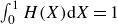 $\int _{0}^{1}H(X){\rm d}X=1$
. This equation indicates that the mass of the liquid film is conserved during the process of electrohydrodynamic patterning.
Nonlinear terms are considered in this model. The geometry of the template is assumed as follows: D(X) = D
0 + 0.5 ΔD tanh [cos(2πX)/B], where B is a positive parameter that controls the wall steepness. The rectangular topography is approximated by a smooth function, and B is taken to be 0.1 in this study. Instead of pursuing an analytical solution, (5.3) is solved by the implementation of a numerical algorithm through the finite difference method (see Appendix B for details). Thus, for a given set of parameters (D
0, ΔD,
 $\varepsilon $
r
, Bo
E
and
 $\overline{A}$
), the profile of the liquid film H(X) can be computed. It is worth mentioning that the lubrication approximation is adopted for both linear model and nonlinear model. This approximation would introduce some errors. However, the errors due to lubrication approximation are acceptable (see Appendix C for details).
Equation (5.3) is a nonlinear equation, and it may have multiple solutions, i.e. multiple equilibrium states, for the given set of parameters (Liu et al. Reference Liu, Ouchi, Jin, Hayward and Suo2019). To obtain all the possible solutions, the numerical model is enhanced by the arclength continuation method (Doedel & Oldeman Reference Doedel and Oldeman1998; Thiele et al. Reference Thiele, Velarde, Neuffer and Pomeau2001, Reference Thiele, Neuffer, Pomeau and Velarde2002, Reference Thiele, Brusch, Bestehorn and Bär2003; Merkt et al. Reference Merkt, Pototsky, Bestehorn and Thiele2005). Equation (5.3) can be rewritten as a function of Bo
E
and H, namely
 $G(Bo_{E},H)=0$
, where
 $G(Bo_{E},H)={(\partial ^{2}H)}/{(\partial X^{2})} + Bo_{E}[(\varepsilon _{r}-1)H-\varepsilon _{r}D] + \overline{A}[({1}/{H^{3})}-({1}/{((D-H)^{3})}]$
. By assuming that one solution of the function is known as
 $G(Bo_{E,0},H_{0})=0$
, then the next solution could be predicted by solving the following set of equations:
 \begin{equation} \left\{\begin{array}{l} G\left(Bo_{E,1},H_{1}\right)=0\\ \left\| H_{1}-H_{0}\right\| + \left| Bo_{E,1}-Bo_{E,0}\right| =\Delta s \end{array}\right. \end{equation}
where H
1 is the interfacial morphology for the electric Bond number Bo
E,1,
 $\| (\boldsymbol{\cdot} )\|$
represents the module of a vector,
 $| (\boldsymbol{\cdot} )|$
denotes the absolute value and Δs refers to the step length that controls the distance between the two adjacent solutions H
0 and H
1. This iterative procedure generates a family of surfaces H for different electric Bond numbers.
By using this nonlinear numerical model, the deformation can be calculated for the given parameters. Figure 3(a) illustrates the dependence of the structure height ΔH on the electric Bond number Bo
E
. For comparison, the linear results are also depicted (the hollow circles in figure 3
a). The nonlinear results are consistent with the linear ones when the deformation is small (
 $\Delta$
H < 0.5). According to the nonlinear numerical results, the Bo
E
∼ ΔH curve takes an ‘S’ shape. When Bo
E
is small, the structure height ΔH increases with the Bo
E
. At a critical value Bo
E,c1 = 1.98, the equilibrium state corresponds to a structure with a relatively large deformation. Actually, the liquid film makes direct contact with the upper template (see point C in figure 3
b). A further increase of the Bo
E
leads to the spreading of the liquid on the template and the thinning of the residual layer at the bottom. Owing to the disjoining pressure, the liquid film is constrained between the upper template and the bottom substrate. The disjoining pressure successfully ensures that the liquid film does not penetrate the solid template.
Nonlinear numerical results of the electrohydrodynamic patterning. (a) Depiction of the relationship between the structure height
 $\Delta$
H and the electric bond number Bo
E
. The hollow circles represent the linear results. (b) The typical deformation of the electrohydrodynamic patterning.

If the Bo E is decreased, the liquid film keeps attaching to the template until the value of Bo E,c2 = 1.5 (see point D in figure 3 b). This effect indicates that once the liquid film attaches the template, a relatively smaller Bo E can maintain the large deformation. If Bo E is in the interval of [Bo E,c2, Bo E,c1], multiple equilibrium states can be observed. The Bo E ∼ ΔH curve takes different paths by increasing/decreasing the Bo E value. When Bo E is increased, the path is A → B → C, while if Bo E is decreased, the path is C → D → A. This behaviour indicates hysteresis in electrohydrodynamic patterning, a phenomenon commonly observed in nonlinear systems (Sherwood Reference Sherwood1988; Behjatian & Esmaeeli Reference Behjatian and Esmaeeli2015; De Ruiter et al. Reference De Ruiter, Semprebon, Van Gorcum, Duits, Brinkmann and Mugele2015). Yeoh et al. (Reference Yeoh, Xu and Basaran2007) conducted pioneering work on the numerical simulation of electrohydrodynamic patterning and studied the equilibrium deformation by the finite element method. Despite differences in configuration, the essential mechanism is the same. Their results are similar to figure 3(a). In their model, the disjoining pressure is not considered. Therefore, only a part of the curve (O → A → B → D) is obtained and the rest part (D → C and hereafter) is missed.
For the hysteresis phenomenon, it is unclear whether it is universal in the electrohydrodynamic patterning. To investigate this, the impact of two parameters, namely the electrical permittivity ratio
 $\varepsilon $
r
and the template-substrate distance D
0, are systematically studied. By varying the electrical permittivity ratio
 $\varepsilon $
r
, it can be seen that the hysteresis phenomenon exists for a larger
 $\varepsilon $
r
. However, the hysteresis phenomenon disappears when
 $\varepsilon $
r
= 2 (figure 4
a). The template-substrate distance D
0 is considered as another parameter that may affect the hysteresis phenomenon. The two critical electric Bond numbers (Bo
E,c1 and Bo
E,c2) are monitored for different D
0 and
 $\varepsilon $
r
values (figure 4
b). If these two Bond numbers are different, hysteresis occurs. If these two numbers coincide, the hysteresis vanishes. As is revealed by figure 4(b), at large D
0 and
 $\varepsilon $
r
a notable hysteresis is observed. By tracking the points where solid lines and dotted lines intersect, a phase diagram is constructed (figure 4
c). In the D
0 ∼
 $\varepsilon $
r
parameter space, the upper-right-hand region corresponds to the cases exhibiting hysteresis, while the lower-left-hand region stands for the cases without it.
Impact of the electrical permittivity ratio
 $\varepsilon $
r
and the structure height
 $\Delta$
H on the deformation. (a) The relationship between the structure height
 $\Delta$
H and the electric bond number Bo
E
with different
 $\varepsilon $
r
values. (b) The dependence of the critical electric bond numbers Bo
E,c1 and Bo
E,c2 on the template-substrate distance D
0 with different
 $\varepsilon $
r
values. (c) The phase diagram of hysteresis deformation. Here Y stands for the existence of hysteresis deformation and N for the no hysteresis phenomenon.

5.1. Lyapunov functional
As shown in the previous section, multiple equilibrium states are formed when Bo
E
∈ [Bo
E,c2, Bo
E,c1], and only one equilibrium state exists if Bo
E
< Bo
E,c2 or Bo
E
> Bo
E,c1. This phenomenon is investigated from the free energy viewpoint. Essentially, (5.1) is regarded as a Cahn–Hilliard-type equation. Correspondingly, a Lyapunov functional can be defined as
 $F=\int _{0}^{1}f{\rm d}X$
, where the energy density f can be expressed by the following equation (Dietzel & Troian Reference Dietzel and Troian2009, Reference Dietzel and Troian2010; Wu, Kavousanakis & Russel Reference Wu, Kavousanakis and Russel2010):
 \begin{equation} f=\frac{1}{2}\left(\nabla H\right)^{2}-Bo_{E}\frac{\left[\varepsilon _{r}\left(D_{0}-H_{0}\right) + H_{0}\right]^{3}}{2\left(\varepsilon _{r}-1\right)\left[\varepsilon _{r}\left(D-H\right) + H\right]} + \frac{\overline{A}}{2}\left[\frac{1}{H^{2}} + \frac{1}{\left(D-H\right)^{2}}\right]. \end{equation}
The first term originates from surface energy, and the second one refers to electrostatic energy. As far as the third term is concerned, it can be regarded as free energy due to a disjoining pressure effect. It is worth noting that the second term has a negative sign. The reason is that an external electrical source is required to power the electrohydrodynamic patterning. When the free energy is calculated, the value needs to add the electrostatic energy and subtract the work done by the externally applied electrical source.
Using the free energy framework, (5.1) can be transformed into the following form:
 \begin{equation} \frac{{\rm d}F}{{\rm d}\tau }=-\int H^{3}\left(\nabla \frac{\delta f}{\delta H}\right)^{2}{\rm d}X .\end{equation}
The Lyapunov functional can be considered as the free energy of the system, and (5.1) represents a spatial–temporal evolution, which minimises the energy. If the parameters Bo
E
,
 $\varepsilon $
r
, D(X) and the interface profile H(X) are specified, then the free energy F can be calculated. It is worth mentioning that (5.1) is essentially the same as (6.2). The former one describes the evolution of liquid film from the viewpoint of force, and the latter one is from the energy. The pressure is essentially the variation of the free energy density with respect to the interface profile,
 $p^{*}=-\delta f/\delta H$
, where
 $p^{*}=p\lambda ^{2}/\gamma {h_{0}}^{2}$
is the non-dimensional pressure.
For a given Bo
E
, the dependence of the free energy F on the structure height
 $\Delta$
H is illustrated in figure 5. When the electric Bond number is relatively small, Bo
E
< Bo
E,c2, one minimum in the free energy can be detected, which corresponds to the stable equilibrium state of the electrohydrodynamic patterning (figure 5
a). If Bo
E,c2 ≤ Bo
E
≤ Bo
E,c1, two minima in the free energy (points P and Q) and one maximum (point O) in the free energy (figures 5
b and 5
c) can be found. Each point corresponds to one equilibrium state: point P corresponds to the equilibrium state that lies in segment AB in figure 3(a), point O refers to segment BD, and point Q denotes DC. At point O, the free energy is maximal and thus, the equilibrium state is unstable. Among the two points P and Q, one of them represents the stable state and the other the metastable. The stable state corresponds to the one that has the lower free energy. If the electric Bond number is further increased, namely Bo
E
> Bo
E,c1, there is only one minimum (point P in figure 5
d), and it corresponds to the stable equilibrium state.
The dependence of the free energy on the structure height
 $\Delta$
H under different electric bond numbers Bo
E
: (a) Bo
E
< Bo
E,c2; (b,c) Bo
E,c2 ≤ Bo
E
≤ Bo
E,c1; (d) Bo
E
> Bo
E,c1.

Figure 5 suggests the existence of an additional critical electric Bond number, where the free energies at P and Q are equal. By calculating the free energy at different electric Bond numbers, the third critical value is found to be Bo
E,c3 = 1.68. This value lies in between the first and second electric Bond number Bo
E,c2 < Bo
E,c3 < Bo
E,c1. At this electric Bond number, the dependence of the free energy on the structure height
 $\Delta$
H is illustrated in figure 6(a). The free energy at point P is indeed equal to that at point Q.
The stability analysis for the multiple equilibrium states. (a) The dependence of the free energy on the structure height
 $\Delta$
H when Bo
E
= Bo
E,c3 = 0.42. (b) The stability of the equilibrium states. (c) The free energy for each equilibrium state (Bo
E
,
 $\Delta$
H) and the equilibrium state is denoted by the Bo
E
.

Based on the free energy, the equilibrium states can be divided into three types: stable, unstable and metastable. In figure 3(a), the equilibrium states (Bo
E
,
 $\Delta$
H) have been obtained. The Bo
E
∼
 $\Delta$
H curve is redrawn according to the stability (figure 6
b). When Bo
E
< Bo
E,c2 or Bo
E
> Bo
E,c1, there is one equilibrium state, and it is stable. When Bo
E,c2 ≤ Bo
E
≤ Bo
E,c1, there are three equilibrium states at the most. As is illustrated in figure 3(a), each equilibrium state lies in the lower (AB), middle (BD) and upper branches (DC) correspondingly. When Bo
E,c2 ≤ Bo
E
≤ Bo
E,c3, the equilibrium state in the lower branch is stable and that in the upper one is metastable (figure 6
b). If Bo
E,c3 < Bo
E
≤ Bo
E,c1, the equilibrium state in the upper branch is stable and that in the lower one is metastable. For the middle branch, it is always unstable. According to the Maxwell stability criterion (Huo & Müller Reference Huo and Müller1993; Hunt, Peletier & Wadee Reference Hunt, Peletier and Wadee2000), a slightly disturbance would trigger the system jump from the metastable equilibrium (local energy minimum) to the stable equilibrium (global energy minimum). When Bo
E
= Bo
E,c3, the free energy at point P equals to that at point Q, thus there are two stable equilibria. The state where the energies of two stable equilibria are equal is commonly referred to as the Maxwell point (Sachkov Reference Sachkov2008).
To further validate the stability of equilibrium states, the free energy F is calculated. For each Bo E , one or multiple equilibrium states can be obtained. For each equilibrium state, the free energy is calculated, and the relationship between Bo E ∼ F is shown in figure 6(c). The major trend is that the free energy decreases with Bo E . However, when Bo E,c2 ≤ Bo E ≤ Bo E,c1, there are multiple free energies since multiple equilibrium states exist. The lowest free energy corresponds to the stable state (green curve), the highest free energy corresponds to the unstable state (red curve) and the intermediate to the metastable state (blue curve).
In the previous sections, the results reveal that the values of critical electric Bond numbers depend on the permittivity ratios (see figure 4). It is reasonable to hypothesise that the permittivity ratio also affects the stability of the equilibrium state. For two permittivity ratios,
 $\varepsilon $
r
= 10 and
 $\varepsilon $
r
= 2, the dependence of free energy F on the electric Bond number Bo
E
is studied (figure 7). When
 $\varepsilon $
r
= 10, the result is similar with the case in figure 6(c). However, the critical electric Bond numbers are significantly decreased. In the present case, Bo
E,c2 = 0.34, Bo
E,c3 = 0.55 and Bo
E,c1 = 0.85. If
 $\varepsilon $
r
= 2, there appears no hysteresis deformation and no critical electric Bond numbers (see figure 4
a). In this circumstance, the free energy decreases monotonously with the electric Bond numbers (figure 7
b). It indicates that all the equilibrium states are stable.
The dependence of the free energy on the electric bond number Bo
E
under different permittivity ratios: (a)
 $\varepsilon $
r
= 10; (b)
 $\varepsilon $
r
= 2.

Equilibrium deformation of the 3-D electrohydrodynamic patterning by the linear model. (a) Depiction of the 3-D template and configuration. (b) The geometry of the equilibrium deformation of the liquid–air interface when
 $\varepsilon $
r
>1. (c) The geometry of the equilibrium deformation of the liquid–air interface when
 $\varepsilon $
r
<1. The colour bar indicates the height of liquid–air interface.

5.2. Three-dimensional deformation of the electrohydrodynamic patterning
In the above sections, the geometry of the liquid–air interface is 2-D, and corresponds to the case of a template with periodic grooves. Another frequently used template in the experiments is the one with periodic square prisms (figure 8 a). For this case, the template is 3-D, and the geometries of the template and the liquid–air interface depend on X and Y, which can be written as follows: D(X, Y) and H(X, Y). The governing equation (5.2) can be extended to the following form:
 \begin{equation} \nabla \boldsymbol{\cdot} \left\{H^{3}Bo_{E}\nabla \left[\varepsilon _{r}D-\left(\varepsilon _{r}-1\right)H\right]-H^{3}\nabla \left(\nabla ^{2}H\right) + \overline{A}H^{3}\nabla \left[\frac{1}{\left(D-H\right)^{3}}-\frac{1}{H^{3}}\right]\right\}=0 \end{equation}
where
 $\nabla =({\partial }/{\partial X},{\partial }/{\partial Y})$
. One period with the size [1 × 1] is considered as the computational domain, and the size of the prism is assumed as [0.5 × 0.5 × 1]. At the boundaries of the computational domain, the following symmetric boundary conditions are imposed:
 ${\partial H}/{\partial X}=0$
and
 ${\partial H}/{\partial Y}=0$
.
A linear model is firstly considered, where the geometries of the template and the liquid–air interface can be expressed as follows:
 \begin{equation} \left\{\begin{array}{l} D(X,Y)\approx D_{0} + \dfrac{1}{\pi }\Delta D\cos \left(2\pi X\right) + \dfrac{1}{\pi }\Delta D\cos \left(2\pi Y\right)\\[9pt] H(X,Y)\approx 1-\dfrac{H_{1}}{2}\cos \left(2\pi X\right)-\dfrac{H_{1}}{2}\cos \left(2\pi Y\right) \end{array}\right. \!.\end{equation}
By substituting into (7.1) and neglecting disjoining pressure and also the higher-order terms, the deformation of the liquid–air interface can be obtained. It is found that the structure height is the same as in the 2-D case (see Appendix D for details). The dependence of the structure height
 $\Delta$
H on the electric Bond number Bo
E
is the same as in figure 2. Also, a critical electric Bond number Bo
E,c
= 4π2/(
 $\varepsilon $
r
− 1) exists. On top of that, when the electric Bond number approaches the critical value, the structure height goes to infinity. As far as the geometry of the liquid–air interface is concerned, some typical results are depicted in figure 8. When
 $\varepsilon $
r
>1, the structure height is positive, indicating a positive replica to the template, and the structure height increases with the electric Bond number Bo
E
(figure 8
b). If
 $\varepsilon $
r
<1, the structure in the liquid film is a negative replica of the template (figure 8
c).
A nonlinear model is also proposed for the 3-D electrohydrodynamic patterning. Following the same procedure in the 2-D case, integrating (7.1) twice, one has
 \begin{equation} \nabla ^{2}H + Bo_{E}\left[\left(\varepsilon _{r}-1\right)H-\varepsilon _{r}D\right] + \overline{A}\left[\frac{1}{H^{3}}-\frac{1}{\left(D-H\right)^{3}}\right]=C_{4} \end{equation}
where C
4 is a constant. The first, second and third terms on the left-hand side represent the Laplace pressure originating from the surface tension, the pressure due to electrical force and the disjoining pressure, respectively. On the right-hand side, the term denotes the hydrostatic pressure. The mass conservation equation, i.e.
 $\int _{0}^{1}\int _{0}^{1}H(X,Y)dXdY=1$
, is required to enable the numerical solution. With the application of the nonlinear model enhanced by the arclength continuation method, (7.3) can be solved by using the finite difference numerical algorithm (see Appendix E for details).
For a set of given parameters, the geometry of the liquid–air interface H(X, Y) can be obtained. The structure height
 $\Delta$
H = max(H) − min(H) is recorded, and the dependence of
 $\Delta$
H on the electric Bond number Bo
E
is illustrated in figure 9(a). Similar to the 2-D case, the
 $\Delta$
H ∼ Bo
E
takes an ‘S’ shape. Two critical electric Bond numbers exist, namely Bo
E,c1 = 1.76, and Bo
E,c2 = 1.4. When Bo
E
∈ [Bo
E,c2, Bo
E,c1], there are multiple equilibrium states. For the geometry of the liquid–air interface, some typical results are depicted in figure 9(b). Hysteresis is also observed in the deformation. Depending on whether electric Bond number is increased or decreased, the interface may acquire different geometries. However, these phenomena are similar to the 2-D case.
Nonlinear numerical results of the 3-D electrohydrodynamic patterning. (a) The relationship between the structure height
 $\Delta$
H and the electric bond number Bo
E
. (b) Some typical deformation of the electrohydrodynamic patterning.

5.3. Concluding remarks
In summary, a linear model and a nonlinear numerical model were proposed for the equilibrium state of the electrohydrodynamic patterning. With the lubrication approximation, the deformation of liquid film can be obtained. According to the foregoing results, the main conclusions may be summarised below.
-
(i) In the linear model, all the higher-order terms are truncated and only the zeroth- and the first-order terms are kept. An equation was successfully obtained which explicitly indicates the relationship between the equilibrium deformation and other parameters. According to this equation, the equilibrium deformation is closely dependent on the electric Bond number Bo E . Interestingly, when the Bond number approaches a critical value, the liquid film deforms remarkably. Based on the linear model, the critical electric Bond number is theoretically predicted Bo E,c = 4π2/(
 $\varepsilon $
r
− 1). To achieve large deformations in micropatterns/nanopatterns, the applied electric Bond number must exceed this value.
-
(ii) The disjoining pressure was included to prevent liquid film penetration, enabling the model to describe the ‘contact’ case between the liquid film and the template. Both models reveal the existence of a critical electric Bond number though the linear model tends to overpredict this value. The nonlinear model shows that the relationship between the deformation amplitude ΔH and electric Bond number Bo E follows an ‘S’ curve, with two critical values Bo E , c1 and Bo E , c2. When the Bo E reaches Bo E , c1, the liquid film deforms significantly and contacts the top template. Once the film attaches to the template, a relatively smaller Bo E can maintain the deformation. The liquid film would not detach until the electric Bond number decreases to Bo E , c2 (usually Bo E , c2 < Bo E , c1). The nonlinear model revealed a hysteresis phenomenon of electrohydrodynamic patterning. Different structures can be obtained by increasing/decreasing the Bo E , namely, multiple equilibrium states can be detected for a given Bo E when Bo E ∈ [Bo E , c2, Bo E , c1].
-
(iii) The stability of the equilibrium states was analysed using the Lyapunov functional, proposed basing on the nonlinear numerical model. By calculating the energy of the system, it was found that when Bo E < Bo E , c2 or Bo E > Bo E , c1, there is one equilibrium state. This state is stable and corresponds to the free energy minimum. When Bo E ∈ [Bo E , c2, Bo E , c1], there are multiple equilibrium states (three at most), among which one is stable, the other is metastable and the third one is unstable.
-
(iv) At the end, the mathematical models (both linear and nonlinear) were extended to 3-D cases. For the 3-D linear case, the deformation amplitude of liquid film ΔH is the same as the 2-D case, if the prism on the 3-D template is square. As for the 3-D nonlinear case, the results are similar with the 2-D case. However, the critical electric Bond numbers predicted by 3-D model are smaller than the 2-D case.
-
(v) Since light is shed on the equilibrium state, the viscosity has no influence on the film deformation. The equilibrium deformation is determined by the delicate balance of electrical stress and surface tension (the disjoining pressure may come into play when the liquid film approaches the top template or substrate). In this paper, the configuration of electrohydrodynamic patterning is assumed as a liquid–air film. The findings are also applicable to the liquid–liquid film.
-
(vi) A straightforward extension of this work could be a study of situations when multiple liquid layers are present. Another possible extension is the case where liquid film has finite conductivity. For this case, the leaky dielectric model rather than the perfect dielectric model, should be used to describe the electrohydrodynamic behaviours. Another direction is to consider the surface wettability (contact angle) as it affects the liquid film morphology after it ‘contacts’ the top template and/or bottom substrate.

Funding
The work was financially supported by the National Natural Science Foundation of China (52175547, U21A20337, 12225208) and the Zhejiang Provincial Natural Science Foundation of China (LMS25E050018). Q.Y. also acknowledges the support of the K. C. Wong Education Foundation.
Declaration of interests
The authors report no conflict of interest.
Appendix A. The effect of the Hamaker constant
In the nonlinear model, the disjoining pressure is introduced which is expressed as
 $p_{m}=A(d-h)^{-3}-Ah^{-3}$
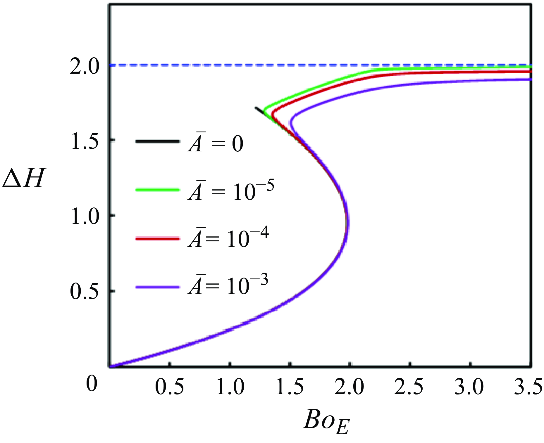
, where A is the Hamaker constant. Essentially, the disjoining pressure indicates that there are two repulsive forces, one is between the liquid film and the upper template, and the other is between the film and the substrate. The purpose of introducing the disjoining pressure is to prevent the penetration. In this appendix, we study the effect of Hamaker constant on the liquid–air interface. As indicated in the main text, the Hamaker constant is characterised by the non-dimensional parameter
 $\overline{A}=A\lambda ^{2}/\gamma {h_{0}}^{4}$
, which denotes the relative importance of disjoining pressure and Laplace pressure caused by the surface tension.
Four different values of
 $\overline{A}$
are tested, and the other parameters are chosen as the default values (see § 4 in the main text). The obtained results are illustrated in figure 10. For a given Bo
E
, the structure height
 $\Delta$
H can be obtained. If the Hamaker constant is zero (
 $\overline{A}=0$
), the disjoining pressure is absent. The steady state cannot be obtained after the point [1.2, 1.7]. In this circumstance, the liquid film has contacted the bottom substrate. Since the repulsive force between liquid film and substrate is absent, the penetration cannot be avoided. Therefore, a zero
 $\overline{A}$
leads to an incomplete Bo
E
∼
 $\Delta$
H curve. For a non-zero
 $\overline{A}$
, the contact case can be modelled and the entire Bo
E
∼
 $\Delta$
H curve can be obtained. The criterion for choosing the value of
 $\overline{A}$
is that the disjoining pressure is negligible when the liquid–air interface is far away from the substrate and template, and the disjoining pressure becomes significant when the interface approaches the substrate or template. If the value of
 $\overline{A}$
is large (see
 $\overline{A}$
= 10−3 in figure 10), the structure height is significantly affected by
 $\overline{A}$
. When
 $\overline{A}$
is decreased to 10−5, it requires more computing time to achieve the converged result. Therefore,
 $\overline{A}$
= 10−4 is used in this study.
The effect of Hamaker constant on the equilibrium deformation of liquid–air interface.

Appendix B. Numerical scheme of the 2-D electrohydrodynamic patterning
For the 2-D nonlinear model, the deformation of liquid film is governed by (5.3) which expresses it as follows:
 \begin{equation} \frac{\partial ^{2}H}{\partial X^{2}} + Bo_{E}\left[\left(\varepsilon _{r}-1\right)H-\varepsilon _{r}D\right] + \overline{A}\left[\frac{1}{H^{3}}-\frac{1}{\left(D-H\right)^{3}}\right]=C_{3}. \end{equation}
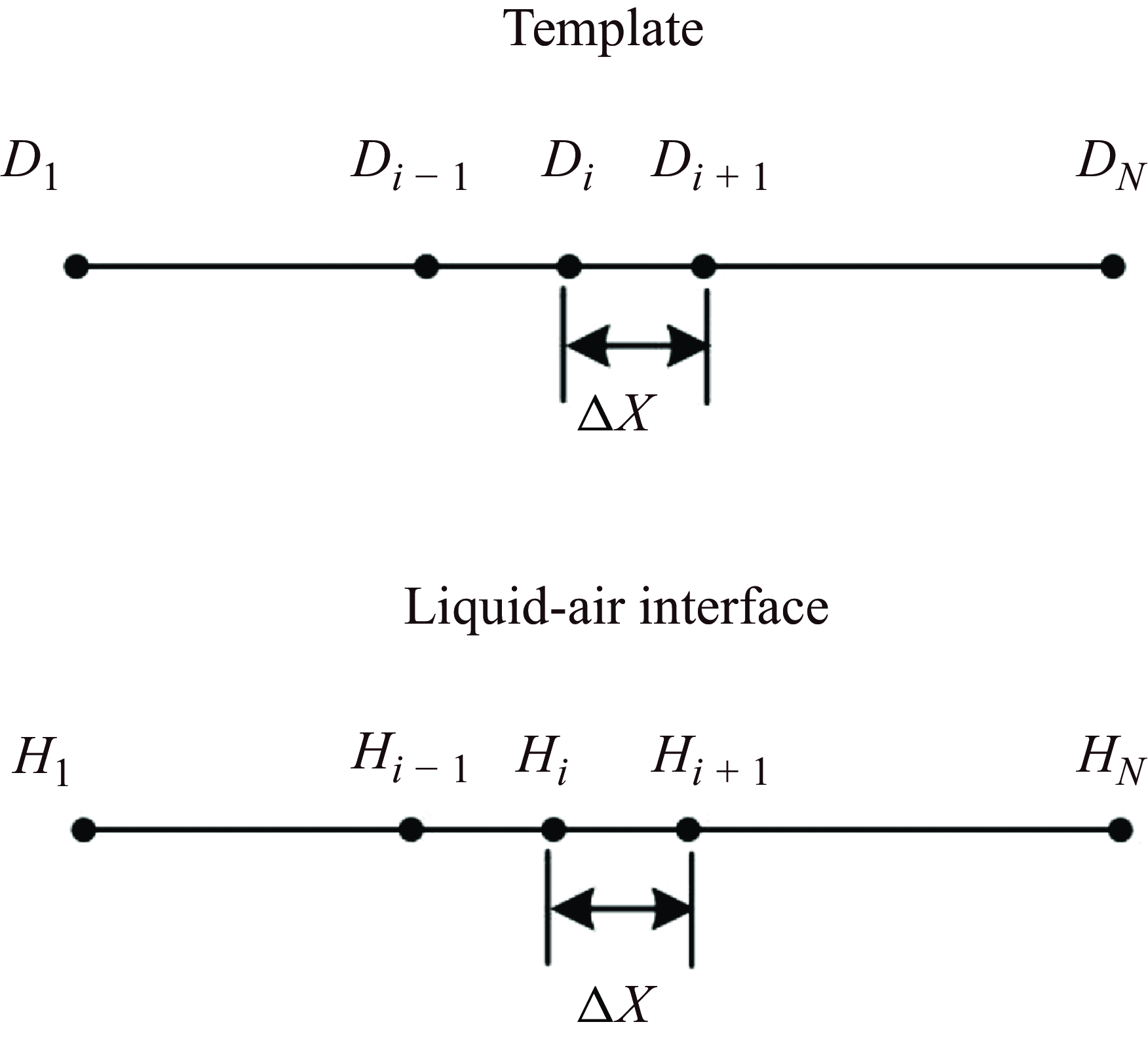
To solve (B1) with the associated boundary conditions, the finite difference method is employed. The computational domain is divided into N−1 elements (figure 11). The nodal points on the template are denoted by D
i
(
 $i=1$
, 2, …, N), and the points on the liquid–air interface are represented by H
i
(
 $i=1$
, 2, …, N). The governing equation can be discretised at the nodal point, which is expressed as
Discretisation of the computational domain.

 \begin{align} 2H_{i}-H_{i + 1}-H_{i-1}&=Bo_{E}\Delta X^{2}\left[\varepsilon _{r}D_{i}-\left(\varepsilon _{r}-1\right)H_{i}\right] + \overline{A}\Delta X^{2}\left[\frac{1}{\left(D_{i}-H_{i}\right)^{3}}-\frac{1}{{H_{i}}^{3}}\right]\nonumber\\&\quad + C_{3} \end{align}
where
 $\Delta$
X is the length of element, and
 $i=2$
, 3, …, N−1. At the first (
 $i=1$
) and the end (
 $i=N$
) nodal points, the boundary condition is ∂H/∂X = 0. The discretised governing equation at these two nodal points can be written as
 \begin{equation} 2H_{1}-2H_{2}=Bo_{E}\Delta X^{2}\left[\varepsilon _{r}D_{1}-\left(\varepsilon _{r}-1\right)H_{1}\right] + \overline{A}\Delta X^{2}\left[\frac{1}{\left(D_{1}-H_{1}\right)^{3}}-\frac{1}{{H_{1}}^{3}}\right] + C_{3}, \end{equation}
 \begin{align} 2H_{N}-2H_{N-1}&=Bo_{E}\Delta X^{2}\left[\varepsilon _{r}D_{N}-\left(\varepsilon _{r}-1\right)H_{N}\right] + \overline{A}\Delta X^{2}\left[\frac{1}{\left(D_{N}-H_{N}\right)^{3}}-\frac{1}{{H_{N}}^{3}}\right]\nonumber\\&\quad + C_{3}.\end{align}
Since C
3 is unknown, an extra equation is required to enable the solution,
 $\int _{0}^{1}H(X)dX=1$
, which indicates the mass is conserved during the process. This equation can be discretised as
 \begin{equation} \frac{H_{1} + H_{N}}{2} + \sum _{i=2}^{N-1}H_{i}=\frac{1}{\Delta X}. \end{equation}
To solve (B2), the under-relaxation iteration method is employed. For a given electric Bond number Bo E , the deformation starts to iterate from the flat interface H i (0) = 1. For the kth iteration, the iterative equation becomes
 \begin{align} 2\overline{H}_{i}^{(k)}-\overline{H}_{i-1}^{(k)}-\overline{H}_{i + 1}^{(k)}-C_{3}&=Bo_{E}\Delta X^{2}\left[\varepsilon _{r}D_{i}-\left(\varepsilon _{r}-1\right)H_{i}^{(k-1)}\right]\nonumber\\&\quad + \overline{A}\Delta X^{2}\left[\frac{1}{\left(D_{i}-H_{i}^{(k-1)}\right)^{3}}-\frac{1}{{H_{i}^{(k-1)}}^{3}}\right] \end{align}
where the symbol H denotes the liquid–air interface and
 $\overline{H}$
the temporary variable. The superscript k indicates the kth iteration, and the subscript i indicates the value at the ith nodal points. The interface H is updated by the following equation:
 \begin{equation} H_{i}^{\left(k\right)}=\omega \overline{H}_{i}^{\left(k\right)} + \left(1-\omega \right)H_{i}^{\left(k-1\right)} \end{equation}
where ω is the relaxation factor and its value is chosen as
 $\omega \in (0,1)$
. The above iteration process is repeated until it converges.
One concern regarding the numerical scheme is that the electric field is discontinuous at the edges of the groove, since the geometry of template D(X) has a sharp corner. The governing equation for film deformation is (5.2). For the rectangular geometry of the template,
 ${\textrm{d}D}/{\textrm{d}X}$
becomes extremely large. However, we did not find any problem when performing the numerical computation. The possible reason is that, after discretisation,
 ${\textrm{d}D}/{\textrm{d}X}$
is in the scale of
 ${\textrm{d}D}/{\textrm{d}X}\sim {D_{2}-D_{1}}/{\Delta X}$
, which is a large value when
 $\Delta X$
is small. This term, however, does not cause the term
 $H_{2}-H_{1}$
to go to infinity. After discretisation,
 ${\text{d}^{3}H}/{\textrm{d}X^{3}}\sim {H_{2}-H_{1}}/{(\Delta X)^{3}}$
. If we balance these two terms,
 ${\textrm{d}D}/{\textrm{d}X}\sim {\text{d}^{3}H}/{\text{d}X^{3}}$
, we have
 $H_{2}-H_{1}\sim (D_{2}-D_{1})\Delta X^{2}$
. Therefore, the jump of D(X) does not cause a jump of H(X).
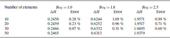
To ensure the accuracy of the numerical model, different element numbers are employed to study the liquid–air interface deformation. The element number is chosen as 10, 20, 30 and 50, respectively. As for the electric Bond number, three values are chosen, Bo E = 1.0, 1.8 and 2.5. Using the numerical algorithm developed in the above section, the deformation of liquid–air interface can be obtained. As indicated in figure 12, the numerical results are insensitive to the element number. To quantify the influence of element number on the deformation, the structure height ΔH is calculated for different element numbers and electric Bond numbers (see table 1 for the results). For each result, the numerical error is calculated by comparing with the case of 50 elements. As revealed in table 1, the numerical errors decrease with the increase of element number. When the element number is 30, the numerical error is less than 0.6%. Therefore, element number 30 is chosen in this study for the numerical simulation.
The effect of element numbers on the numerical results of liquid–air interface deformation. The electric bond numbers are (a) Bo E = 1.0, (b) 1.8 and (c) 2.5.


Appendix C. The justification of the Lubrication approximation
In this paper, the long-wave approximation (i.e. lubrication approximation) is adopted in order to enable the analytical solution of governing equations. Both linear and nonlinear models take this approximation, namely the periodic length λ is much larger than the film thickness h 0. However, the introduction of such an approximation would cause some errors. In this appendix, the error caused by the long-wave approximation is studied. We choose the electric potential at the liquid–air interface as the test parameter. For electrohydrodynamic patterning, the electric field is governed by the Laplace equation (see (3.1)). With the boundary conditions, the equation can be numerically solved without the long-wave approximation by some commercial software. We use COMSOL Multiphysics (v6.0) for the numerical solution, and the module ‘Electrostatics’ is selected.
With the long-wave approximation, the electric potential at the liquid–air can be expressed as (see (3.2))
 \begin{equation} V=\frac{V_{0}h}{\varepsilon _{r}d-\left(\varepsilon _{r}-1\right)h}. \end{equation}
In the linear model, the boundary of top template is expressed as
 $d=d_{0} + {2}/{\pi }\Delta d\cos (2\unicode{x03C0} x/\lambda )$
, where d
0 is the distance between the substrate and top template,
 $\Delta$
d is the structure height of top template and λ is the periodic length. In the nonlinear model,
 $d=d_0$
+ 0.5 Δd tanh [cos(2πx/λ)/ B], where B is a positive parameter that controls the wall steepness, and it is chosen as 0.1 in this study. If the liquid–air interface h is specified, then the electric potential V can be calculated.
The liquid–air interface is taken as h = h
0+0.5
 $\Delta$
h cos(2πx/λ), where h
0 is the initial thickness of liquid film,
 $\Delta$
h is the structure height. Three cases are considered,
 $\Delta$
 $h=0$
, 0.6 h
0 and 1.2 h
0, which correspond to a flat interface, an interface with a small deformation, and an interface with a large deformation. The other parameters are the same as in the main text. The electric potential can be obtained by three models, namely, the linear model, the nonlinear model and the numerical model. For a comparison, the results from all these three models are depicted together in figure 13. Compared with the numerical results, the linear model over-predicts the electric potential at the middle part and under-predicts the potential at the two sides. Overall, these three models are consistent with each other.
The electric potential along the liquid–air interface by the linear, nonlinear and fully numerical models. (a) The interface is flat y = h 0. (b) The interface with a small deformation y = h 0 + 0.3 h 0 cos(2πx/λ). (c) The interface with a large deformation y = h 0 + 0.6 h 0 cos(2πx/λ).

The discrepancy between the linear and numerical models is measured by
 $e_{lin}=\sqrt{\sum _{i=1}^{N}(V_{lin,i}-V_{num,i})^{2}/{V_{0}}^{2}N}$
, where V
lin,i
is the electric potential at x
i
by the linear model, and V
num i
by the numerical model, V
0 is the applied voltage, N the total number of nodal points. Similarly, the discrepancy between the nonlinear model and the numerical one is defined by
 $e_{non}=\sqrt{\sum _{i=1}^{N}(V_{non,i}-V_{num,i})^{2}/{V_{0}}^{2}N}$
where V
non,i
is the electric potential at x
i
by the nonlinear model. For the three cases shown in figure 14, namely the flat interface y = h
0, slightly deformed interface y = h
0 + 0.3 h
0 cos(2πx/λ), and largely deformed interface y = h
0+0.6 h
0 cos(2πx/λ), the error of the linear model is 3.36%, 3.50% and 6.22%. As for the error of nonlinear model, it is 3.41%, 2.94% and 4.11%, respectively.
The error of the linear and nonlinear models compared with the fully numerical model. (a) The error of the linear model e lin . (b) The error of the nonlinear model e non .

The 3-D electrohydrodynamic patterning. (a) The configuration and (b) the computational domain.

To identify the region where the linear and nonlinear models with lubrication approximations are consistent with the numerical one, the effect of parameters on the errors e
lin
and e
non
are studied. Special interest is focused on the effect of the following parameters: the deformation of liquid–air interface (structure height
 $\Delta$
H =
 $\Delta$
h/h
0), the wavelength (λ/h
0) and the dielectric constant
 $\varepsilon $
r
. As illustrated in figure 14, the errors of linear model and nonlinear model become smaller with the increase of wavelength λ/h
0. The reason is that both linear model and nonlinear model are based on the long-wave approximation (lubrication approximation). Overall, the errors (both linear and nonlinear models) are smaller than 10% within the parameter space,
 $\Delta$
H ∈ [0, 1.2], λ/h
0 ∈ [1, 10],
 $\varepsilon $
r
∈ [2, 10].
Appendix D. The linear model for the 3-D template
For the 3-D electrohydrodynamic patterning, the configuration and computational domain are illustrated in figure 15. The template is topographical with periodic prisms, and only one period is chosen as the computational domain. The size of the computational domain is [0, λ
x
]×[0, λ
y
]×[0, d
0+
 $\Delta$
d/2]. The size of prism is
 $\Delta d\times\alpha\lambda_x \times\beta\lambda_y $
, where
 $\alpha$
∈ [0, 1] and
 $\beta$
∈ [0, 1].
Using the Fourier series, the geometry of template d(x, y) and liquid–air interface h(x, y) are approximated as
 \begin{equation} \left\{\begin{array}{l} d(x,y)\approx d_{0} + \left(\dfrac{1}{2}-\alpha \beta \right)\Delta d + \dfrac{2\beta }{\pi }\Delta d\sin \left(\alpha \pi \right)\cos \left(\dfrac{2\pi x}{\lambda _{x}}\right)\\\quad\quad\quad\quad + \dfrac{2\alpha }{\pi }\Delta d\sin \left(\beta \pi \right)\cos \left(\dfrac{2\pi y}{\lambda _{y}}\right)\\ h(x,y)\approx h_{0}-h_{1}\cos \left(\dfrac{2\pi x}{\lambda _{x}}\right)-h_{2}\cos \left(\dfrac{2\pi y}{\lambda _{x}}\right) \end{array}\right. \!.\end{equation}
The characteristic length in the x, y and z directions is chosen as λ x , λ x and h 0, where h 0 is the initial thickness of liquid film. The above equation can be written as
 \begin{equation} \left\{\begin{array}{l} D(X,Y)\approx D_{0} + \left(\dfrac{1}{2}-\alpha \beta \right)\Delta D + \dfrac{2\beta }{\pi }\Delta D\sin \left(\alpha \pi \right)\cos \left(2\pi X\right)\\\quad\quad\ \quad\quad + \dfrac{2\alpha }{\pi }\Delta D\sin \left(\beta \pi \right)\cos \left(2\pi Y\dfrac{\lambda _{x}}{\lambda _{y}}\right)\\ H(X,Y)\approx 1-H_{1}\cos \left(2\pi X\right)-H_{2}\cos \left(2\pi Y\dfrac{\lambda _{x}}{\lambda _{y}}\right) \end{array}\right. \!.\end{equation}
Substituting the D(X) and H(X) into (7.3), and ignoring the molecular forces, one can get the expression for H 1 and H 2:
 \begin{equation} \left\{\begin{array}{l} H_{1}=\dfrac{2\beta \varepsilon _{r}\Delta D\sin \left(\alpha \pi \right)}{4\pi ^{3}B{o_{E}}^{-1}-\pi \left(\varepsilon _{r}-1\right)}\\[11pt] H_{2}=\dfrac{2\alpha \varepsilon _{r}\Delta D\sin \left(\beta \pi \right)}{4\pi ^{3}B{o_{E}}^{-1}\left(\lambda _{x}/\lambda _{y}\right)^{2}-\pi \left(\varepsilon _{r}-1\right)}. \end{array}\right. \end{equation}
As for the structure height, it can be calculated by
 $\Delta$
H = 2H
1+2H
2. The structure height goes to infinity if either H
1 or H
2 is infinity (the denominator approaches zero).
Some special cases are considered. If
 $\alpha=1/2$
and
 $\beta=1$
, the template simplifies into the 2-D geometry as illustrated in figure 1. In this case,
 $H_{1}={2\varepsilon _{r}\Delta D}/{4\pi ^{3}B{o_{E}}^{-1}-\pi (\varepsilon _{r}-1)}$
, H
2 = 0, and the structure height becomes (4.2). If
 $\alpha \neq 1$
and
 $\beta \neq 1$
, then the template takes a 3-D geometry. We consider a special case, the period in x direction equals that in y direction, λ
x
= λ
y
. The structure height in this case can be written as
 \begin{equation} \Delta H=\frac{4C_{g}\varepsilon _{r}\Delta D}{4\pi ^{3}B{o_{E}}^{-1}-\pi \left(\varepsilon _{r}-1\right)} \end{equation}
where
 $C_{g}=\beta \sin (\alpha \pi ) + \alpha \sin (\beta \pi )$
is referred to as the geometry factor. Equation (D4) is similar to (4.2) but with the geometry factor C
g
. The dependence of C
g
on
 $\alpha$
and
 $\beta$
is illustrated in figure 16. The minimum of C
g
is 0, and C
g
achieves its maximum value of 1.16 when
 $\alpha$
=
 $\beta$
= 0.65. If the length and width of the prism are half of the period,
 $\alpha$
=
 $\beta$
= 0.5, then C
g
= 1. In this case, (D4) simplifies to (4.2). Therefore, with the given geometry
 $\alpha$
=
 $\beta$
= 0.5, the structure height in 3-D case is identical to that in 2-D case.
The dependence of geometry factor C g on the length and width of the prism.

Appendix E. Numerical scheme of the 3-D electrohydrodynamic patterning
The governing equation of 3-D electrohydrodynamic patterning is (7.3), which is expressed as follows:
 \begin{equation} \nabla ^{2}H + Bo_{E}\left[\left(\varepsilon _{r}-1\right)H-\varepsilon _{r}D\right] + \overline{A}\left[\frac{1}{H^{3}}-\frac{1}{\left(D-H\right)^{3}}\right]=C_{4}. \end{equation}
The numerical scheme is similar with the 2-D case. The computational domain is divided into (N−1) × (N−1) elements. The nodal points on the template are denoted by D i, j (i = 1, 2, …, N and j = 1, 2, …, N), and the points on the liquid–air interface are represented by H i, j (i = 1, 2, …, N and j = 1, 2, …, N). The governing equation can be discretised at the nodal point, which is expressed as
 \begin{equation} \begin{array}{l} 2H_{i,j}-H_{i + 1,j}-H_{i-1,j} + \dfrac{\Delta X^{2}}{\Delta Y^{2}}\left(2H_{i,j}-H_{i,j + 1}-H_{i,j-1}\right)\\\quad = Bo_{E}\Delta X^{2}\left[\varepsilon _{r}D_{i,j}-\left(\varepsilon _{r}-1\right)H_{i,j}\right] + \overline{A}\Delta X^{2}\left[\dfrac{1}{\left(D_{i,j}-H_{i,j}\right)^{3}}-\dfrac{1}{{H_{i,j}}^{3}}\right] + C_{4} \end{array} \end{equation}
where
 $\Delta$
X and
 $\Delta$
Y are the lengths of element in the x and y directions. In this study,
 $\Delta$
X =
 $\Delta$
Y.
Also, the under-relaxation iteration method is employed to solve (E2). For a given electric Bond number Bo
E
, the deformation starts to iterate from the flat interface
 $H_{i,j}^{(0)}=1$
. For the kth iteration, the iterative equation becomes
 \begin{equation} \begin{array}{l} 4\overline{H}_{i,j}^{\left(k\right)}-\overline{H}_{i-1,j}^{\left(k\right)}-\overline{H}_{i + 1,j}^{\left(k\right)}-\overline{H}_{i,j-1}^{\left(k\right)}-\overline{H}_{i,j + 1}^{\left(k\right)}-C_{4}\\\quad = Bo_{E}\Delta X^{2}\left[\varepsilon _{r}D_{i,j}-\left(\varepsilon _{r}-1\right)H_{i,j}^{\left(k-1\right)}\right] + \overline{A}\Delta X^{2}\left[\dfrac{1}{\left(D_{i}-H_{i,j}^{\left(k-1\right)}\right)^{3}}-\dfrac{1}{{H_{i,j}^{\left(k-1\right)}}^{3}}\right] \end{array} \end{equation}
where the symbol H denotes the liquid–air interface and
 $\overline{H}$
the temporary variable. The superscript k indicates the kth iteration, and the subscripts i, j indicate the values at the (i, j)th nodal points. The interface H is updated by the following equation:
 \begin{equation} H_{i,j}^{\left(k\right)}=\omega \overline{H}_{i,j}^{\left(k\right)} + \left(1-\omega \right)H_{i,j}^{\left(k-1\right)} \end{equation}
where ω is the relaxation factor and its value is chosen as
 $\omega \in (0,1)$
. The above iteration process is repeated until it converges.