1 Introduction
The importance of velocity gradient tensor (VGT) dynamics in turbulent flows has been fully recognised since the works of Taylor (Reference Taylor1938) and Betchov (Reference Betchov1956). These authors established the importance of vortex stretching and strain self-amplification in relation to the turbulence cascade (see Tsinober Reference Tsinober2009). Although their work was limited to homogeneous isotropic turbulence (HIT), they are still relevant for a wider range of turbulent flows that are often only locally homogeneous with isotropic small scales.
In the past three years, a number of authors have started addressing the question of the spatial evolution of VGT statistics and dynamics in grid-generated turbulence (Laizet, Vassilicos & Cambon Reference Laizet, Vassilicos and Cambon2013; Gomes-Fernandes, Ganapathisubramani & Vassilicos Reference Gomes-Fernandes, Ganapathisubramani and Vassilicos2014; Zhou et al.
Reference Zhou, Nagata, Sakai, Suzuki, Ito, Terashima and Hayase2014a
, Reference Zhou, Nagata, Sakai, Ito and Hayase2015, Reference Zhou, Nagata, Sakai, Ito and Hayase2016a
,Reference Zhou, Nagata, Sakai, Ito and Hayase
b
). The question is of course wider and should eventually be addressed in various spatially developing turbulent flows. But grid-generated turbulence (like some other turbulent flows) has two regions: a production region nearest to the grid where the turbulence intensity builds up till it reaches a peak value at a certain distance from the grid (Simmons & Salter Reference Simmons and Salter1934; Warhaft & Jayesh Reference Warhaft1992; Hurst & Vassilicos Reference Hurst and Vassilicos2007; Weitemeyer et al.
Reference Weitemeyer, Reinke, Peinke and Hölling2013); and an immediate adjacent downstream region where the turbulence decays. The question is to know in which region and where within the region different VGT properties of the turbulence originate from and how they might correlate with statistics traditionally attributed to a turbulence cascade, such as the celebrated
 $-5/3$
power-law range of the turbulent energy spectrum.
Experimentally, classical regular grids such as those used by Corrsin and his collaborators (Comte-Bellot & Corrsin Reference Comte-Bellot and Corrsin1966, Reference Comte-Bellot and Corrsin1971) are very difficult to use for this purpose as they are designed in such a way that the production region is very short. The first and to date the only experimental investigation on the subject (Gomes-Fernandes et al.
Reference Gomes-Fernandes, Ganapathisubramani and Vassilicos2014) was therefore done with space-filling fractal square grids where the production region is greatly magnified and therefore more easily accessible. The first direct numerical simulation (DNS) on the subject (Laizet et al.
Reference Laizet, Vassilicos and Cambon2013) was also carried out for space-filling fractal square grids and they showed how the well-known universal teardrop shape of the
 $Q{-}R$
diagram (see Tsinober Reference Tsinober2009) is absent in the grid centreline region where, however, the
 $2/3$
power law for the second-order structure function of the fluctuating velocity is present. Recall that
 $Q$
and
 $R$
are the VGT’s second and third invariants and the
 $Q{-}R$
diagram is the joint probability density function (JPDF) of
 $Q$
and
 $R$
.
A series of DNS studies followed from Nagoya University in Japan (Zhou et al.
Reference Zhou, Nagata, Sakai, Suzuki, Ito, Terashima and Hayase2014a
,Reference Zhou, Nagata, Sakai, Suzuki, Ito, Terashima and Hayase
b
, Reference Zhou, Nagata, Sakai, Ito and Hayase2015, Reference Zhou, Nagata, Sakai, Ito and Hayase2016a
,Reference Zhou, Nagata, Sakai, Ito and Hayase
b
) where the fractal square grid was replaced by a single square element of the fractal grid (which resembles a hollow square plate). A fractal square grid is constructed by replicating this element at various length scales. On the other hand, replicating the element at the same length scale forms a classical grid. Therefore, this is a fundamental building block for both the classical and fractal grids. By replacing the fractal grid with its square element, the production region remains magnified while at the same time isolating the effect of only one of the features of the fractal grid, the largest square pattern. These studies confirmed the appearance of the
 $2/3$
power law in the second-order structure function in the very near field of the grid-element centreline. Other well-known universal properties of the VGT, such as the teardrop shape of the
 $Q{-}R$
diagram and alignments between vorticity and strain-rate eigenvectors (Ashurst et al.
Reference Ashurst, Kerstein, Kerr and Gibson1987; Tsinober Reference Tsinober2009) did also appear quite further downstream. They also showed that the pressure Hessian at the centreline is dominant very close to the element, closer than the point where the
 $2/3$
power law first appears as one moves in the streamwise direction.
A particular observation made by Laizet et al. (Reference Laizet, Vassilicos and Cambon2013) is that the local Reynolds number based on the Taylor length scale (
 $Re_{\unicode[STIX]{x1D706}}$
) can be relatively small where the
 $2/3$
power law first appears. The studies of Zhou et al. (Reference Zhou, Nagata, Sakai, Suzuki, Ito, Terashima and Hayase2014a
,Reference Zhou, Nagata, Sakai, Suzuki, Ito, Terashima and Hayase
b
, Reference Zhou, Nagata, Sakai, Ito and Hayase2015, Reference Zhou, Nagata, Sakai, Ito and Hayase2016a
,Reference Zhou, Nagata, Sakai, Ito and Hayase
b
) showed that the well-known universal turbulence properties of the VGT (
 $Q{-}R$
diagrams, VGT alignments, etc.) are present in the decay region even for values of
 $Re_{\unicode[STIX]{x1D706}}$
as small as 50 or so. An unrelated study by Schumacher et al. (Reference Schumacher, Scheel, Krasnov, Donzis, Yakhot and Sreenivasan2014) which was concerned with periodic turbulence, turbulent shear flow between two parallel walls and thermal convection in a closed container, also identified that some universal turbulence properties of velocity gradients are present even at relatively modest Reynolds numbers.
In light of these publications, the motivation for the present work on velocity gradients in spatially developing flow is threefold. Firstly, to take the observation of Zhou et al. (Reference Zhou, Nagata, Sakai, Ito and Hayase2015) concerning the dominance of the pressure Hessian very close to the grid-element one step further and describe the mechanism of generation of vorticity (components
 $\unicode[STIX]{x1D714}_{i}$
) and strain-rate tensor (components
 $\unicode[STIX]{x1D634}_{ij}$
) along the grid-element centreline and the bar centreline. Secondly, to study VGT statistics at relatively low
 $Re_{\unicode[STIX]{x1D706}}$
to ensure very good spatial resolution of our DNS and to further test and explore the idea that some turbulence statistics do not require high Reynolds numbers to appear. And thirdly, to add to the literature on this subject some hitherto undocumented strain-rate statistics and some comparisons between low Reynolds number turbulence generated by single square grid-element and higher Reynolds number turbulence generated by fractal square grids. The present work reports on DNS of turbulence generated by a single square grid-element and we compare our results wherever possible with the laboratory study of turbulence generated by a space-filling fractal square grid of Gomes-Fernandes et al. (Reference Gomes-Fernandes, Ganapathisubramani and Vassilicos2014) and the DNS results of Zhou et al. (Reference Zhou, Nagata, Sakai, Suzuki, Ito, Terashima and Hayase2014a
,Reference Zhou, Nagata, Sakai, Suzuki, Ito, Terashima and Hayase
b
, Reference Zhou, Nagata, Sakai, Ito and Hayase2015, Reference Zhou, Nagata, Sakai, Ito and Hayase2016a
,Reference Zhou, Nagata, Sakai, Ito and Hayase
b
).
This paper is organised as follows. Details of the grid-element and the computational parameters are given in §§ 2 and 3 respectively. Section 4 validates our solver with the available experimental data. The main findings of this study are discussed in § 5, and the results are summarised in § 6.
2 Geometrical details of the square grid-element
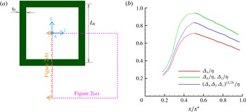
The present DNS deals with the flow past a single square grid-element of fractal grid (or simply a square grid-element). A sketch with the basic dimensions and the coordinate system is shown in figure 1(a). The lateral thickness of the grid-element is
 $t_{0}=43$
mm, while the length is
 $L_{0}=5.3t_{0}=229$
mm. The thickness of the grid bar in the streamwise direction is 6 mm.
The aspect ratio (AR) of the bar, defined as the ratio of the streamwise to the lateral thickness, is 0.14, and not 1.0 as in the case of classical grids. This is because we examine the single square pattern of the fractal square grid whose streamwise thickness is equal to that of the smallest square element. Therefore, this study considers the streamwise thickness of the fractal square grid used in the studies of Gomes-Fernandes, Ganapathisubramani & Vassilicos (Reference Gomes-Fernandes, Ganapathisubramani and Vassilicos2012), Gomes-Fernandes et al. (Reference Gomes-Fernandes, Ganapathisubramani and Vassilicos2014), Laizet, Nedić & Vassilicos (Reference Laizet, Nedić and Vassilicos2015a ,Reference Laizet, Nedić and Vassilicos b ).
(a) Sketch of the single square grid-element and the coordinate system. The dotted box and the dot-dashed cut section are the locations where the computational mesh is shown in figure 2. (b) Mesh resolution along the grid-element centreline normalised with the local length scale,
 $\unicode[STIX]{x1D702}$
, as a function of the normalised streamwise distance from the grid-element.

In the following sections we normalise the streamwise distance with the characteristic wake-interaction length scale,
 $x^{\ast }$
, defined by Mazellier & Vassilicos (Reference Mazellier and Vassilicos2010). In order to derive this length scale, it is assumed that the turbulent wake starts immediately downstream of the bar, and thus the laminar and transitional parts of the wake are neglected. It is known that the wake width of a turbulence generating body of size
 $t_{0}$
grows as
 $\sqrt{t_{0}x}$
in the downstream direction (Townsend Reference Townsend1980). Therefore, the wakes are expected to meet at a downstream streamwise location which scales with
 $x^{\ast }$
where
 $L_{0}\approx \sqrt{t_{0}x^{\ast }}$
, and
 $L_{0}$
is the distance between the parallel bars. From this, one can obtain the wake-interaction length scale based on the grid-element parameters as
 $x^{\ast }=L_{0}^{2}/t_{0}$
.
3 Numerical method and computational parameters
Throughout this paper, instantaneous, mean and fluctuating velocity fields are denoted as
 $u_{i}^{\ast }$
,
 $U_{i}$
and
 $u_{i}$
respectively (where
 $i=1,2,3$
), and the corresponding variables for pressure are
 $p^{\ast }$
,
 $P$
and
 $p$
. The continuity and momentum equations are written as:
 $$\begin{eqnarray}\displaystyle & \displaystyle \frac{\unicode[STIX]{x2202}u_{i}^{\ast }}{\unicode[STIX]{x2202}x_{i}}=0, & \displaystyle\end{eqnarray}$$
 $$\begin{eqnarray}\displaystyle & \displaystyle \frac{\unicode[STIX]{x2202}u_{i}^{\ast }}{\unicode[STIX]{x2202}t}+u_{j}^{\ast }\frac{\unicode[STIX]{x2202}u_{i}^{\ast }}{\unicode[STIX]{x2202}x_{j}}=-\frac{1}{\unicode[STIX]{x1D70C}}\frac{\unicode[STIX]{x2202}p^{\ast }}{\unicode[STIX]{x2202}x_{i}}+\unicode[STIX]{x1D708}\frac{\unicode[STIX]{x2202}^{2}u_{i}^{\ast }}{\unicode[STIX]{x2202}x_{j}\unicode[STIX]{x2202}x_{j}}, & \displaystyle\end{eqnarray}$$
where
 $\unicode[STIX]{x1D70C},\unicode[STIX]{x1D708}$
are the density and kinematic viscosity respectively.
These equations are solved using our in-house parallel code Pantarhei (Lu & Papadakis Reference Lu and Papadakis2011, Reference Lu and Papadakis2014; Papadakis Reference Papadakis2011). This code is an unstructured finite volume solver that uses a collocated variable arrangement. For spatial discretisation of the convective and viscous terms, a second-order central differencing scheme is employed, while the second-order backward differencing scheme is used for the transient term. The convective term is linearised using a second-order extrapolation of the velocity
 $u_{j}^{\ast }$
from the previous two time instants while
 $u_{i}^{\ast }$
is treated implicitly. Viscous terms are also treated fully implicitly. The momentum interpolation method of Rhie & Chow (Reference Rhie and Chow1983) is applied to compute the velocities at the cell faces. The code is parallelised using the PETSc (portable extensive toolkit for scientific computation) libraries (Balay et al.
Reference Balay, Abhyankar, Adams, Brown, Brune, Buschelman, Eijkhout, Gropp, Kaushik and Knepley2014). For the solution of the pressure equation the generalised minimal residual (GMRES) method is used together with the BoomerAMG algebraic multigrid preconditioner of the Hypre package (Falgout & Yang Reference Falgout and Yang2002).


The size of the computational domain is
 $L_{x}\times L_{y}\times L_{z}=7L_{0}\times 2L_{0}\times 2L_{0}$
. The blockage ratio of the single square grid-element is 20 %, which is the same as in the experiments reported in Laizet et al. (Reference Laizet, Nedić and Vassilicos2015a
). The grid-element is placed at a distance
 $1.75L_{0}$
from the inlet of the computational domain, which is sufficiently large compared to previous DNS studies (Laizet et al.
Reference Laizet, Vassilicos and Cambon2013, Reference Laizet, Nedić and Vassilicos2015a
).
The Reynolds number based on the free-stream velocity
 $U_{\infty }$
and the bar length
 $L_{0}$
is
 $Re_{L_{0}}=2650$
, while based on the lateral thickness
 $t_{0}$
is
 $Re_{t_{0}}=500$
. The time step of the simulation is kept constant at
 $0.015U_{\infty }/t_{0}$
, resulting in a maximum Courant–Friedrichs–Levy (CFL) number of 0.47. Uniform velocity is prescribed at the inlet, while a convective outlet boundary condition is used at the exit. No-slip boundary conditions are applied on the walls, while all lateral boundaries are considered to be periodic.
The total number of computational cells are
 $20.4\times 10^{6}$
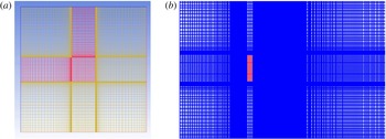
. The mesh is body fitted and the cell faces align exactly with the bar walls. The flexibility offered by the unstructured meshing allows for optimal placement of control volumes. Figure 2 shows the computational mesh for the locations marked in figure 1(a). The distance between the bar surface and the closest mesh point in the wall-normal direction is less than 0.15 wall units (i.e.
 $\unicode[STIX]{x0394}n^{+}<0.15$
). This shows that the boundary layers developing on the bar surfaces are well resolved. The mesh is refined near the walls to resolve the shear layers that develop after separation from the front sharp corners. There are approximately 17 cells inside the shear layer closer to the grid-element (around
 $x/x^{\ast }\approx 0.02$
), while there are approximately 24 cells inside the shear layer thickness around
 $x/x^{\ast }\approx 0.5$
.
In the region where the wakes have met, the resolution of the present mesh is assessed in terms of a local length scale (
 $\unicode[STIX]{x1D702}$
) defined as the square root of the ratio between kinematic viscosity and local standard deviation of fluctuating strain rate, i.e.
 $\unicode[STIX]{x1D702}=\sqrt{\unicode[STIX]{x1D708}/\sqrt{\langle \unicode[STIX]{x1D634}_{ij}\unicode[STIX]{x1D634}_{ij}\rangle }}$
, where
 $\unicode[STIX]{x1D634}_{ij}$
is the turbulent strain rate. This length scale can be used to characterise the spatial extent over which the local velocity gradients are smoothed out by viscosity and is, as such, of general applicability. It actually turns out that this length scale is the same as the Kolmogorov micro-scale (
 $\unicode[STIX]{x1D702}=(\unicode[STIX]{x1D708}^{3}/\unicode[STIX]{x1D716})^{1/4}$
) in the case of fully developed turbulent flows. One can therefore use this length scale to assess mesh resolution wherever there is fluctuating strain, including in the decaying region where the entire field is fully turbulent. Figure 1(b) depicts the variation of ratios between local mesh resolutions
 $\unicode[STIX]{x1D6E5}_{x}$
,
 $\unicode[STIX]{x1D6E5}_{y}$
,
 $\unicode[STIX]{x1D6E5}_{z}$
,
 $\unicode[STIX]{x1D6E5}$
(defined as
 $\unicode[STIX]{x1D6E5}=(\unicode[STIX]{x1D6E5}_{x}\unicode[STIX]{x1D6E5}_{y}\unicode[STIX]{x1D6E5}_{z})^{1/3}$
) and the local length scale,
 $\unicode[STIX]{x1D702}$
for
 $x/x^{\ast }>0.2$
. The dotted lines denote the region where the turbulence is intermittent, and the solid lines represent the fully turbulent decay region. The figure shows that the resolution in all directions is always less than one
 $\unicode[STIX]{x1D702}$
along the grid-element centreline. Resolution requirements for a proper DNS have been reported in Moin & Mahesh (Reference Moin and Mahesh1998), Donzis, Yeung & Sreenivasan (Reference Donzis, Yeung and Sreenivasan2008). The latter authors mention that a standard resolution for the second-order quantities (such as the root-mean-square (r.m.s.) velocities or the energy spectrum which takes very small values and falls off rapidly at wavenumbers
 $k>1/\unicode[STIX]{x1D702}$
) is
 $\unicode[STIX]{x0394}x/\unicode[STIX]{x1D702}\approx 2$
. For higher-order moments of velocity derivatives and velocity increments (for example fourth-order moments) resolution down to the Kolmogorov scale is required. It is expected therefore that the present mesh is sufficiently fine for the computation of all the terms in the balance equations for enstrophy and strain product. Evidence for this is shown in § 5.
The flow is first allowed to develop for 1 flow-through time and then data are collected for 10 flow-through times (or 144 000 time steps) to ensure satisfactory statistical convergence.
4 Comparison with experiments
Figure 3(a) shows instantaneous streamwise velocity contours at plane
 $z/x^{\ast }=0$
. The black and pink dotted-dash lines in the figure represent the grid-element centreline and the bar centreline respectively. The two wakes behind the bars are clearly seen. The wakes are initially separated by a jet that emerges from the gap between the bars, but as the wakes grow downstream, they meet intermittently and begin to interact. This process starts at about
 $x/x^{\ast }\approx 0.2$
. Contours of the time-averaged streamwise velocity are shown in figure 3(b). The flow is highly inhomogeneous in the lee of the grid-element, but as the wakes interact dispersing momentum in the cross-stream direction, it becomes more homogeneous further downstream and is already quite homogeneous at
 $x\approx x^{\ast }$
, in agreement with the experimental observations of Seoud & Vassilicos (Reference Seoud and Vassilicos2007).
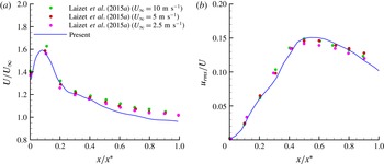
In order to validate our DNS, we compare one-point velocity statistics with the experiments reported in Laizet et al. (Reference Laizet, Nedić and Vassilicos2015a
). Figure 4(a) shows the time-averaged streamwise velocity (
 $U$
) normalised with the free-stream velocity (
 $U_{\infty }$
) along the grid-element centreline. The velocity profile obtained from our DNS solver agrees well with the experimental measurements carried out for Reynolds number at least ten times larger than that of the present study. The velocity profile exhibits a jet-like behaviour close to the grid-element, followed by a monotonic decay in the downstream. Note the strong acceleration (by almost 60 %) of the streamwise velocity compared to
 $U_{\infty }$
in the lee of the grid-element. The velocity profile peaks around
 $x/x^{\ast }\approx 0.1$
(i.e.
 $x/L_{0}\approx 0.5$
), and the velocity peak magnitude is expected to depend on the grid-element blockage and the mesh resolution. For example in the simulations of Laizet et al. (Reference Laizet, Nedić and Vassilicos2015a
), this peak is underestimated by approximately 10 % when the coarsest mesh is employed. The effect of blockage on the acceleration is strong: the square grid-element of Zhou et al. (Reference Zhou, Nagata, Sakai, Suzuki, Ito, Terashima and Hayase2014a
, Reference Zhou, Nagata, Sakai, Ito and Hayase2016a
) has a blockage of 11 % (nearly half compared to ours) and their acceleration is less than 20 %.
Note also that for
 $x/x^{\ast }>0.4$
the simulations underpredict the experiments by approximately 5 %. This can be explained by the difference between the experimental and computational set-ups. As mentioned earlier, all lateral boundaries are periodic in the simulations, while they are solid walls in the experiments. As the wakes expand, they tilt slightly towards the top and bottom boundaries, as seen in figure 3(b). Previous simulations (Zhou et al.
Reference Zhou, Nagata, Sakai, Suzuki, Ito, Terashima and Hayase2014a
) have reported the same finding. In the experiments, the boundary layers that form along the lateral boundaries act as a blockage for the flow. As a result, the mean velocity increases in order to maintain a constant mass flow rate. This leads to a slight underprediction of the experiments. Valente & Vassilicos (Reference Valente and Vassilicos2014) compared the mean and r.m.s. profiles of the wakes interacting with each other as well as with the lateral wall versus the wakes interacting each other in a quasi-periodic arrangement. They reported that the lateral wall surfaces have a meaningful effect on mean and r.m.s. velocity profiles only in the far downstream region (i.e. after
 $x/x^{\ast }>1.25$
as far as the current simulation is concerned). They also found that the location where the bar wakes meet is not altered by differences in the lateral boundaries. Therefore, we impose periodic boundary conditions on the lateral boundaries in order to avoid the large computational cost associated with the resolution of the near-wall region. Note that the previous numerical studies on grid turbulence also have periodic lateral boundaries (Laizet et al.
Reference Laizet, Vassilicos and Cambon2013, Reference Laizet, Nedić and Vassilicos2015a
; Zhou et al.
Reference Zhou, Nagata, Sakai, Suzuki, Ito, Terashima and Hayase2014a
,Reference Zhou, Nagata, Sakai, Suzuki, Ito, Terashima and Hayase
b
, Reference Zhou, Nagata, Sakai, Ito and Hayase2015, Reference Zhou, Nagata, Sakai, Ito and Hayase2016a
,Reference Zhou, Nagata, Sakai, Ito and Hayase
b
).
Contour plots in the
 $x{-}y$
plane at
 $z/x^{\ast }=0$
: (a) instantaneous streamwise velocity, (b) mean streamwise velocity. The isocontours range from 1.8 to
 $-0.75$
in units of
 $U_{\infty }$
. The bar centreline and grid-element centreline are marked by magenta and black dotted-dash lines respectively.

Comparison of (a) mean velocity and (b) streamwise turbulent intensity along the grid-element centreline with measurements.

Figure 4(b) depicts the evolution of the streamwise r.m.s. velocity (
 $u_{rms}$
) normalised by the local mean velocity (not
 $U_{\infty }$
) along the grid-element centreline. The turbulent intensity increases from the lee of the grid-element until
 $x/x^{\ast }\approx 0.5$
. The region between
 $x/x^{\ast }=0$
and
 $x/x^{\ast }=0.5$
is termed the production region, and the location where the turbulent intensity attains its maximum value is called the peak location. After the peak,
 $u_{rms}$
decreases in the decay region. Experiments and predictions match reasonably well. The aforementioned effect of boundary layer growth has been compensated by the normalisation with the local velocity. Note that at
 $x/x^{\ast }=0$
, the predicted r.m.s. value of fluctuating velocity matches well with the experiment (both values are close to 0). This means that no artificial fluctuations are produced by the discretisation method upstream of the grid-element. The growth of r.m.s. velocity from
 $x=0$
to
 $x\approx 0.5x^{\ast }$
is also well predicted. Simulating this region is particularly challenging because the flow transitions from laminar to turbulent as the turbulent/non-turbulent interfaces from the bar wakes sweep this region. The success in correctly simulating this region further demonstrates that the employed mesh resolution is adequate.
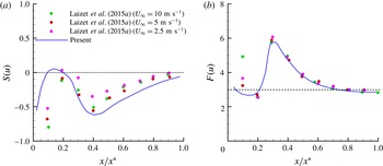
Comparison of (a) skewness and (b) flatness of streamwise fluctuating velocity along the grid-element centreline with experiments.

The skewness and flatness of streamwise velocity fluctuations are presented in figures 5(a) and 5(b) respectively where the values corresponding to Gaussian fluctuating velocities are shown as dotted lines. It can be seen that the turbulence is highly non-Gaussian in the production region, and then slowly returns to Gaussianity further downstream (it is reminded that the skewness and flatness of a Gaussian random variable are 0 and 3 respectively). The comparison with the experiments is (perhaps surprisingly) good, especially for the flatness. The profiles are smooth which indicates good convergence of the statistics. Reynolds number effects are strongest in the location closest to the lee of the grid-element (
 $x/x^{\ast }=0.1$
) and this is the region with the largest deviation from the experiments. Further downstream, there is still some dependence on Reynolds number, especially for the skewness, but for flatness this dependency is weak and the matching with the experiments is significantly better. The skewness of fluctuating velocity
 $S(u)$
is negative and decreases in the production region till
 $x/x^{\ast }\approx 0.4$
. The value of
 $S(u)$
remains non-zero but increases continuously towards zero further downstream in agreement with the simple closure calculation of Maxey (Reference Maxey1987) for a decaying homogeneous turbulence. In the work of Zhou et al. (Reference Zhou, Nagata, Sakai, Suzuki, Ito, Terashima and Hayase2014a
) the largest negative skewness and positive flatness occur around
 $x/x^{\ast }\approx 0.2$
, while in our case they occur later, at
 $x/x^{\ast }\approx 0.4$
. This difference is attributed to the locations where the wakes start to meet. In their low blockage ratio grid-element, the wakes meet at
 $x/x^{\ast }\approx 0.1$
while the wakes meet at
 $x/x^{\ast }\approx 0.2$
in the present case.
Basic turbulence parameters at the six locations considered along the grid-element centreline. Here
 $Re_{\unicode[STIX]{x1D706}}=u_{rms}\unicode[STIX]{x1D706}/\unicode[STIX]{x1D708}$
(
 $\unicode[STIX]{x1D706}$
is the Taylor length scale computed from
 $\unicode[STIX]{x1D706}=\sqrt{u^{2}/(\unicode[STIX]{x2202}u/\unicode[STIX]{x2202}x)^{2}}$
) and
 $S(\unicode[STIX]{x2202}u/\unicode[STIX]{x2202}x)$
is the skewness of the fluctuating streamwise velocity derivative.

We probe all three regions (production, peak and decay) by choosing six different spatial locations along the grid-element centreline. These
 $x/x^{\ast }$
coordinates along with their basic turbulence parameters are provided in table 1. The first three points (with
 $x/x^{\ast }=0.1$
, 0.25 and 0.35) lie inside the production region and have the following characteristics (in the ascending order of
 $x/x^{\ast }$
): point closest to the grid-element; point where a slope close to
 $-5/3$
in the energy spectrum is first observed; point in the production region with similar
 $Re_{\unicode[STIX]{x1D706}}$
as the last point in the decay region. The fourth point (
 $x/x^{\ast }=0.5$
) is located at the turbulence peak. The final two locations (
 $x/x^{\ast }=0.75$
and 0.95) correspond, respectively, to: the point which has the maximum
 $Re_{\unicode[STIX]{x1D706}}$
; and the point in the decay region with about the same
 $Re_{\unicode[STIX]{x1D706}}$
as point 3.
Table 1 also records the values of skewness of fluctuating streamwise velocity derivative,
 $S(\unicode[STIX]{x2202}u/\unicode[STIX]{x2202}x)$
, at all stations. This skewness is very small near the grid-element but in the decay region it attains values which are closer to those reported in the literature for homogeneous turbulence. Indeed, Tavoularis, Corrsin & Bennett (Reference Tavoularis, Corrsin and Bennett1978) reported that the value of
 $S(\unicode[STIX]{x2202}u/\unicode[STIX]{x2202}x)$
lies in the range
 $-0.35$
to
 $-0.45$
for relatively low Reynolds number turbulence, a fact also recorded in the review of Sreenivasan & Antonia (Reference Sreenivasan and Antonia1997). Our results are in line with these values in the decay region where the turbulence is most homogeneous.
5 Results and discussion
We start by studying the characteristics of the flow through the budgets of turbulent kinetic energy, mean enstrophy and mean strain product. Then we proceed to establish the relationship between the small-scale terms and energy spectra along the grid-element centreline. Finally, the invariants of the VGT and geometrical statistics of small-scale turbulence are discussed.
5.1 Budgets of turbulent kinetic energy, enstrophy and strain rate
The symmetric (strain rate) and antisymmetric (vorticity) parts of VGT are analysed through the budgets of mean strain product and mean enstrophy respectively. As a precursor, the budget of mean kinetic energy is discussed first.
5.1.1 Turbulent kinetic energy balance
The transport equation of turbulent kinetic energy is (refer to Tennekes & Lumley Reference Tennekes and Lumley1972),
 $$\begin{eqnarray}\displaystyle \frac{\unicode[STIX]{x2202}}{\unicode[STIX]{x2202}t}\left(\frac{1}{2}\langle u_{i}u_{i}\rangle \right) & = & \displaystyle \underbrace{-U_{j}\frac{\unicode[STIX]{x2202}}{\unicode[STIX]{x2202}x_{j}}\left(\frac{1}{2}\langle u_{i}u_{i}\rangle \right)}_{C_{k}}\underbrace{-\frac{\unicode[STIX]{x2202}}{\unicode[STIX]{x2202}x_{j}}\left(\frac{1}{\unicode[STIX]{x1D70C}}\langle u_{j}p\rangle \right)}_{\unicode[STIX]{x03C0}_{k}}\nonumber\\ \displaystyle & & \displaystyle \underbrace{-\frac{\unicode[STIX]{x2202}}{\unicode[STIX]{x2202}x_{j}}\left(\frac{1}{2}\langle u_{i}u_{i}u_{j}\rangle \right)}_{T_{k}}\underbrace{+\frac{\unicode[STIX]{x2202}}{\unicode[STIX]{x2202}x_{j}}(2\unicode[STIX]{x1D708}\langle u_{i}\unicode[STIX]{x1D634}_{ij}\rangle )}_{D_{k}}\underbrace{-\langle u_{i}u_{j}\rangle \unicode[STIX]{x1D61A}_{ij}}_{P_{k}}\underbrace{-2\unicode[STIX]{x1D708}\langle \unicode[STIX]{x1D634}_{ij}\unicode[STIX]{x1D634}_{ij}\rangle }_{\unicode[STIX]{x1D716}_{k}},\end{eqnarray}$$
where
 $\unicode[STIX]{x1D634}_{ij}$
and
 $\unicode[STIX]{x1D61A}_{ij}$
are the fluctuating and mean strain rates respectively,
 $$\begin{eqnarray}\displaystyle & \displaystyle \unicode[STIX]{x1D634}_{ij}=\frac{1}{2}\left(\frac{\unicode[STIX]{x2202}u_{i}}{\unicode[STIX]{x2202}x_{j}}+\frac{\unicode[STIX]{x2202}u_{j}}{\unicode[STIX]{x2202}x_{i}}\right), & \displaystyle\end{eqnarray}$$
 $$\begin{eqnarray}\displaystyle & \displaystyle \unicode[STIX]{x1D61A}_{ij}=\frac{1}{2}\left(\frac{\unicode[STIX]{x2202}U_{i}}{\unicode[STIX]{x2202}x_{j}}+\frac{\unicode[STIX]{x2202}U_{j}}{\unicode[STIX]{x2202}x_{i}}\right). & \displaystyle\end{eqnarray}$$
In (5.1),
 $C_{k}$
denotes the convection due to mean flow,
 $\unicode[STIX]{x03C0}_{k}$
represents the pressure work,
 $T_{k}$
corresponds to the transport by fluctuations,
 $D_{k}$
stands for viscous diffusion, the production of turbulent kinetic energy by mean flow is
 $P_{k}$
and the dissipation of turbulent kinetic energy is denoted by
 $\unicode[STIX]{x1D716}_{k}$
.
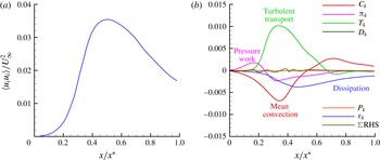
(a) Evolution of turbulent kinetic energy along the grid-element centreline. (b) Turbulent kinetic energy budget along the grid-element centreline (all terms are normalised by
 $U_{\infty }^{3}/t_{0}$
).

The streamwise evolution of turbulent kinetic energy along the grid-element centreline is shown in figure 6(a). In the production region, the turbulent kinetic energy increases from zero to a peak value. This increase is gradual for
 $x/x^{\ast }<0.2$
where the flow is mostly irrotational, and steeper for
 $0.2\leqslant x/x^{\ast }\leqslant 0.4$
where the turbulence is developing. The kinetic energy decreases in the decay region (i.e. for
 $x/x^{\ast }>0.5$
).
The budget of turbulent kinetic energy along the grid-element centreline is depicted in figure 6(b) where all the terms in (5.1) are normalised by
 $U_{\infty }^{3}/t_{0}$
. For statistically stationary flows, as the one considered in this paper, the transient term on the left-hand side is zero. Figure 6(b) shows that the grid-element centreline turbulent kinetic energy budget is markedly different from some previously reported budgets for boundary layer (Mansour, Kim & Moin Reference Mansour, Kim and Moin1988) and backward facing step (Le, Moin & Kim Reference Le, Moin and Kim1997). The distinguishing feature here is the absence of production term,
 $P_{k}$
. The turbulent kinetic energy along the grid-element centreline is not the result of mean-flow gradients producing turbulent fluctuations, as in wall-bounded shear flows. In the region
 $0\leqslant x/x^{\ast }<0.2$
, the rise of energy is due mainly to pressure work. As we show in the next section, this part of the grid-element centreline is dominated by irrotational flow. Around
 $x/x^{\ast }\approx 0.2$
, the transport by turbulent fluctuations becomes the term responsible for the turbulent kinetic energy growth. This is the direct result of wakes starting to reach the grid-element centreline and meet around that location and thereby transporting turbulent kinetic energy towards the grid-element centreline. From
 $x/x^{\ast }\approx 0.2$
to the end of the production region, transport by fluctuations is counteracted by viscous dissipation, pressure work and mean advection. At the start of the decay region, the mean-flow advection term changes its sign and is mainly balanced by viscous dissipation in most of the decay region. The budget analysis reveals that the flow along the grid-element centreline is initially irrotational and becomes turbulent due to lateral infiltration of turbulent wakes from the grid-element bars.
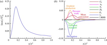
(a) Evolution of turbulent kinetic energy along the bar centreline. (b) Turbulent kinetic energy budget along the bar centreline (all terms are normalised by
 $U_{\infty }^{3}/t_{0}$
).

The turbulent kinetic energy profile along the bar centreline is given in figure 7(a). The turbulent intensity increases up to
 $x/x^{\ast }\approx 0.13$
along the bar centreline due to the deformation of the Reynolds stress tensor by the mean velocity gradients (production term,
 $P_{k}$
) and the pressure work,
 $\unicode[STIX]{x03C0}_{k}$
(refer to figure 7
b). Notice that
 $P_{k}$
is now the dominant term, but
 $\unicode[STIX]{x03C0}_{k}$
is still important. The contribution of
 $P_{k}$
would have been even stronger if the budget analysis was performed along the core of the shear layer emanating from the top (or the bottom) face of the bar. This region has the strongest strain rate, refer to figure 3. Near the bar,
 $P_{k}$
and
 $\unicode[STIX]{x03C0}_{k}$
are balanced by the sum of turbulent transport and dissipation. Further downstream, the mean turbulent kinetic energy starts to decay as the contribution of pressure work and mean velocity gradients decrease. In the far downstream (i.e. after
 $x/x^{\ast }>0.4$
), the mean flow carries the turbulent kinetic energy, and it is balanced by dissipation. Figures 6(b) and 7(b) also show that the mean turbulent kinetic energy equation is properly balanced in our simulations.
5.1.2 Mean enstrophy balance
The transport equation for mean enstrophy
 $\langle \unicode[STIX]{x1D714}_{i}\unicode[STIX]{x1D714}_{i}\rangle$
is given by (refer to Tennekes & Lumley Reference Tennekes and Lumley1972),
 $$\begin{eqnarray}\displaystyle \frac{\unicode[STIX]{x2202}}{\unicode[STIX]{x2202}t}\left(\frac{1}{2}\langle \unicode[STIX]{x1D714}_{i}\unicode[STIX]{x1D714}_{i}\rangle \right) & = & \displaystyle \underbrace{-U_{j}\frac{\unicode[STIX]{x2202}}{\unicode[STIX]{x2202}x_{j}}\left(\frac{1}{2}\langle \unicode[STIX]{x1D714}_{i}\unicode[STIX]{x1D714}_{i}\rangle \right)}_{C_{\unicode[STIX]{x1D714}}}\underbrace{-\langle u_{j}\unicode[STIX]{x1D714}_{i}\rangle \frac{\unicode[STIX]{x2202}\unicode[STIX]{x1D6FA}_{i}}{\unicode[STIX]{x2202}x_{j}}}_{G_{\unicode[STIX]{x1D714}}}\nonumber\\ \displaystyle & & \displaystyle \underbrace{-\frac{1}{2}\frac{\unicode[STIX]{x2202}}{\unicode[STIX]{x2202}x_{j}}\langle u_{j}\unicode[STIX]{x1D714}_{i}\unicode[STIX]{x1D714}_{i}\rangle }_{T_{\unicode[STIX]{x1D714}}}\underbrace{+\langle \unicode[STIX]{x1D714}_{i}\unicode[STIX]{x1D714}_{j}\unicode[STIX]{x1D634}_{ij}\rangle }_{P_{\unicode[STIX]{x1D714}}}\underbrace{+\langle \unicode[STIX]{x1D714}_{i}\unicode[STIX]{x1D714}_{j}\rangle \unicode[STIX]{x1D61A}_{ij}}_{\unicode[STIX]{x1D6FC}_{\unicode[STIX]{x1D714}}}\underbrace{+\langle \unicode[STIX]{x1D714}_{i}\unicode[STIX]{x1D634}_{ij}\rangle \unicode[STIX]{x1D6FA}_{j}}_{\unicode[STIX]{x1D6FD}_{\unicode[STIX]{x1D714}}}\nonumber\\ \displaystyle & & \displaystyle \underbrace{+\unicode[STIX]{x1D708}\frac{\unicode[STIX]{x2202}^{2}}{\unicode[STIX]{x2202}x_{j}\unicode[STIX]{x2202}x_{j}}\left\langle \frac{1}{2}\unicode[STIX]{x1D714}_{i}\unicode[STIX]{x1D714}_{i}\right\rangle }_{\unicode[STIX]{x1D708}_{\unicode[STIX]{x1D714}}}\underbrace{-\unicode[STIX]{x1D708}\left\langle \frac{\unicode[STIX]{x2202}\unicode[STIX]{x1D714}_{i}}{\unicode[STIX]{x2202}x_{j}}\frac{\unicode[STIX]{x2202}\unicode[STIX]{x1D714}_{i}}{\unicode[STIX]{x2202}x_{j}}\right\rangle }_{\unicode[STIX]{x1D716}_{\unicode[STIX]{x1D714}}},\end{eqnarray}$$
where
 $\unicode[STIX]{x1D714}_{i}$
and
 $\unicode[STIX]{x1D6FA}_{i}$
are the components of the vorticity vector of the fluctuating and time-averaged fields respectively and are given by
 $$\begin{eqnarray}\displaystyle & \displaystyle \unicode[STIX]{x1D714}_{i}=\unicode[STIX]{x1D716}_{ijk}\frac{\unicode[STIX]{x2202}u_{k}}{\unicode[STIX]{x2202}x_{j}}, & \displaystyle\end{eqnarray}$$
 $$\begin{eqnarray}\displaystyle & \displaystyle \unicode[STIX]{x1D6FA}_{i}=\unicode[STIX]{x1D716}_{ijk}\frac{\unicode[STIX]{x2202}U_{k}}{\unicode[STIX]{x2202}x_{j}}, & \displaystyle\end{eqnarray}$$
where
 $\unicode[STIX]{x1D716}_{ijk}$
is the Levi-Civita symbol. In (5.4)
 $C_{\unicode[STIX]{x1D714}}$
is the advection by mean flow,
 $G_{\unicode[STIX]{x1D714}}$
represents the production by mean field,
 $T_{\unicode[STIX]{x1D714}}$
is the transport by turbulent fluctuations,
 $P_{\unicode[STIX]{x1D714}}$
is the enstrophy production by stretching of fluctuating strain rate,
 $\unicode[STIX]{x1D6FC}_{\unicode[STIX]{x1D714}}$
corresponds to production (or removal) of enstrophy by stretching (or squeezing) due to mean strain rate,
 $\unicode[STIX]{x1D6FD}_{\unicode[STIX]{x1D714}}$
is the mixed production term while
 $\unicode[STIX]{x1D708}_{\unicode[STIX]{x1D714}}$
and
 $\unicode[STIX]{x1D716}_{\unicode[STIX]{x1D714}}$
represent viscous diffusion and dissipation of enstrophy respectively.
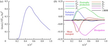
(a) Evolution of mean enstrophy along the grid-element centreline. (b) Budget of mean enstrophy along the grid-element centreline (all terms are normalised by
 $(U_{\infty }/t_{0})^{3}$
).

The profile of mean enstrophy along the grid-element centreline is depicted in figure 8(a). In the lee of the grid-element (
 $x/x^{\ast }<0.2$
) the enstrophy is almost zero. Therefore, the flow in this part of the grid-element centreline maybe considered irrotational, which also implies non-turbulent. The mean enstrophy increases slowly after
 $x/x^{\ast }>0.2$
and it continues to increase until the turbulence peak at
 $x/x^{\ast }=0.5$
. Further downstream in the decay region, the enstrophy continuously decreases.
Further physical insight on the observed variation of enstrophy can be gained from the budget of enstrophy (figure 8
b). Every term in equation (5.4) is normalised by
 $(U_{\infty }/t_{0})^{3}$
. The budget demonstrates that all the terms are nearly zero for the irrotational flow part of the grid-element centreline (i.e. for
 $x/x^{\ast }<0.2$
). Moving further from this location, the first term in space to contribute to the generation of mean enstrophy is the turbulent transport term,
 $T_{\unicode[STIX]{x1D714}}$
. The physical mechanism, therefore, is clear: vorticity, which is produced at the grid-element surface due to the no-slip boundary condition, is first shed into bar wakes and then transported towards the grid-element centreline through the bar wakes that disperse vorticity in the lateral directions. Vorticity reaches the grid-element centreline at
 $x/x^{\ast }\approx 0.2$
. Interestingly, the skewness and flatness (shown in figure 5) are close to their Gaussian values of 0 and 3 respectively exactly at this point, and deviate from them further downstream in the production region. In particular, the skewness becomes negative which indicates the presence of strong negative fluctuations. These decelerations correlate with the intermittent interaction between the two wakes in the part of production region where
 $x/x^{\ast }\approx 0.2$
(see Melina, Bruce & Vassilicos (Reference Melina, Bruce and Vassilicos2016) for further information on this point).
Shortly after the action of
 $T_{\unicode[STIX]{x1D714}}$
, the other terms in the transport equation start to become active. For example, after
 $x/x^{\ast }=0.25$
, the fluctuating strain field stretches the (small amount of) existing transported vorticity causing further production of enstrophy (
 $P_{\unicode[STIX]{x1D714}}$
term). Both
 $T_{\unicode[STIX]{x1D714}}$
,
 $P_{\unicode[STIX]{x1D714}}$
are positive leading to the very rapid growth of
 $\langle \unicode[STIX]{x1D714}_{i}\unicode[STIX]{x1D714}_{i}\rangle$
(figure 8
a). These two terms are balanced by advection due to mean flow and viscous dissipation.
Turbulent and mean transport terms grow in the production region but are reduced to small values at the peak location. Further downstream in the decay region,
 $P_{\unicode[STIX]{x1D714}}$
and
 $\unicode[STIX]{x1D716}_{\unicode[STIX]{x1D714}}$
become the dominant terms that balance each other. It is worth mentioning here that the terms involving mean velocity gradients do not contribute to the transport of enstrophy anywhere on the grid-element centreline even in the production region, although this region is highly inhomogeneous.
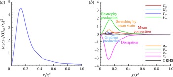
(a) Evolution of mean enstrophy along the bar centreline. (b) Budget of mean enstrophy along the bar centreline (all terms are normalised by
 $(U_{\infty }/t_{0})^{3}$
).

Figure 9 illustrates the dynamics of fluctuating enstrophy along the bar centreline. The mean enstrophy profile (figure 9
a) appears to be qualitatively similar to that of the bar centreline turbulent kinetic energy with values peaking at the same location
 $x/x^{\ast }\approx 0.13$
. Figure 9(b) reveals that once the vorticity is shed into the bar wake, it is continuously stretched by the fluctuating strain rate throughout the bar centreline. Close to the bar, the increase in mean enstrophy is mostly because of the vortex stretching (
 $P_{\unicode[STIX]{x1D714}}$
term). Mechanisms such as the stretching of vorticity by mean strain (
 $\unicode[STIX]{x1D6FC}_{\unicode[STIX]{x1D714}}$
), and the production due to mean vorticity gradients (
 $G_{\unicode[STIX]{x1D714}}$
) also contribute to the growth of enstrophy in the near-bar region although their contribution is small compared to that of the vortex stretching. Further downstream, the vortex stretching term is in balance with the dissipation of enstrophy, and all other terms are negligible (figure 9
b). Although the mean and turbulent transport terms are the significant budget terms along the grid-element centreline, their contribution to the mean enstrophy budget is minimum along the bar centreline. This budget analysis also shows that the mixed production term (
 $\unicode[STIX]{x1D6FD}_{\unicode[STIX]{x1D714}}$
) does not contribute to the transport of mean enstrophy along both the grid-element centreline and the bar centreline.
Tennekes & Lumley (Reference Tennekes and Lumley1972) predicted that
 $P_{\unicode[STIX]{x1D714}}$
and
 $\unicode[STIX]{x1D716}_{\unicode[STIX]{x1D714}}$
are the dominant terms in (5.4). Their prediction appears to be valid on the bar centreline. On the grid-element centreline, however, our DNS reveals that the turbulent and mean transport terms are also equally important, in particular in the production region. All other terms are predicted to be significantly smaller by Tennekes & Lumley (Reference Tennekes and Lumley1972) and our simulation confirms that they are indeed negligible.
The balancing of mean enstrophy equation (figures 8 b and 9 b), while not absolutely perfect, is definitely within acceptable limits. Our choice of low Reynolds number has been essential in achieving this and it is the first time such a point balance is reported in a study of a spatially developing flow. For channel flow it has been reported by Sandham & Tsinober (Reference Sandham and Tsinober2000).
5.1.3 Mean strain-product balance
The transport equation for mean strain product
 $\langle \unicode[STIX]{x1D634}_{ij}\unicode[STIX]{x1D634}_{ij}\rangle$
is (refer to Tsinober Reference Tsinober2009),
 $$\begin{eqnarray}\displaystyle \frac{\unicode[STIX]{x2202}}{\unicode[STIX]{x2202}t}\left(\frac{1}{2}\langle \unicode[STIX]{x1D634}_{ij}\unicode[STIX]{x1D634}_{ij}\rangle \right) & = & \displaystyle \underbrace{-U_{k}\frac{\unicode[STIX]{x2202}}{\unicode[STIX]{x2202}x_{k}}\left(\frac{1}{2}\langle \unicode[STIX]{x1D634}_{ij}\unicode[STIX]{x1D634}_{ij}\rangle \right)}_{C_{s}}\underbrace{-\langle u_{k}\unicode[STIX]{x1D634}_{ij}\rangle \frac{\unicode[STIX]{x2202}\unicode[STIX]{x1D61A}_{ij}}{\unicode[STIX]{x2202}x_{k}}}_{\unicode[STIX]{x1D6FC}_{s}}\nonumber\\ \displaystyle & & \displaystyle \underbrace{-\frac{1}{2}\frac{\unicode[STIX]{x2202}}{\unicode[STIX]{x2202}x_{k}}\langle u_{k}\unicode[STIX]{x1D634}_{ij}\unicode[STIX]{x1D634}_{ij}\rangle }_{T_{s}}\underbrace{-2\langle \unicode[STIX]{x1D634}_{ij}\unicode[STIX]{x1D634}_{ik}\rangle \unicode[STIX]{x1D61A}_{kj}}_{\unicode[STIX]{x1D6FD}_{s}}\underbrace{-\frac{1}{2}\langle \unicode[STIX]{x1D714}_{i}\unicode[STIX]{x1D634}_{ij}\rangle \unicode[STIX]{x1D6FA}_{j}}_{\unicode[STIX]{x1D708}_{s}}\underbrace{-\langle \unicode[STIX]{x1D634}_{ij}\unicode[STIX]{x1D634}_{jk}\unicode[STIX]{x1D634}_{ki}\rangle }_{P_{s}}\nonumber\\ \displaystyle & & \displaystyle \underbrace{-\frac{1}{4}\langle \unicode[STIX]{x1D714}_{i}\unicode[STIX]{x1D714}_{j}\unicode[STIX]{x1D634}_{ij}\rangle }_{\unicode[STIX]{x1D714}_{s}}\underbrace{-\left\langle \unicode[STIX]{x1D634}_{ij}\frac{\unicode[STIX]{x2202}^{2}p}{\unicode[STIX]{x2202}x_{i}\unicode[STIX]{x2202}x_{j}}\right\rangle }_{\unicode[STIX]{x03C0}_{s}}\underbrace{+\unicode[STIX]{x1D708}\langle \unicode[STIX]{x1D634}_{ij}\unicode[STIX]{x1D6FB}^{2}\unicode[STIX]{x1D634}_{ij}\rangle }_{\unicode[STIX]{x1D716}_{s}},\end{eqnarray}$$
where
 $C_{s}$
is the mean-flow advection,
 $\unicode[STIX]{x1D6FC}_{s}$
is the production by mean strain field,
 $T_{s}$
is the turbulent transport,
 $\unicode[STIX]{x1D6FD}_{s}$
is the production due to stretching by mean strain rate,
 $\unicode[STIX]{x1D708}_{s}$
is the mixed production term,
 $P_{s}$
is the production due to stretching by fluctuating strain field (also known as the strain self-amplification term). The enstrophy production term (
 $\unicode[STIX]{x1D714}_{s}$
) also appears in the transport equation of mean strain product but with a negative sign and premultiplied by (
 $-1/4$
),
 $\unicode[STIX]{x03C0}_{s}$
is the strain pressure Hessian correlation term and
 $\unicode[STIX]{x1D716}_{s}$
is the viscous dissipation term.
(a) Evolution of mean strain product along the grid-element centreline. (b) Budget of mean strain product along the grid-element centreline (all terms are normalised by
 $(U_{\infty }/t_{0})^{3}$
).

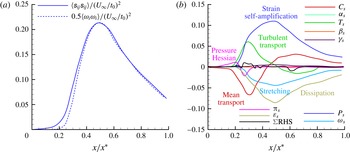
Figure 10(a) depicts the profile of mean strain product along the grid-element centreline. The profile of
 $0.5\langle \unicode[STIX]{x1D714}_{i}\unicode[STIX]{x1D714}_{i}\rangle$
is also plotted in the same figure. Although the flow in the vicinity of grid-element (
 $x/x^{\ast }<0.2$
) does not contain any significant enstrophy, it does possess strain (figure 10
a). The dissipation of turbulent kinetic energy is directly proportional to the strain product,
 $\unicode[STIX]{x1D716}_{k}=2\unicode[STIX]{x1D708}\langle \unicode[STIX]{x1D634}_{ij}\unicode[STIX]{x1D634}_{ij}\rangle$
, so this is a region of mostly irrotational dissipation. The strain increases rapidly after
 $x/x^{\ast }>0.2$
until the peak region, and then decreases in the decay region. Note that
 $0.5\langle \unicode[STIX]{x1D714}_{i}\unicode[STIX]{x1D714}_{i}\rangle \approx \langle \unicode[STIX]{x1D634}_{ij}\unicode[STIX]{x1D634}_{ij}\rangle$
is not valid in the production region (see also table 3). Recall that in homogeneous turbulence it is straightforward to prove analytically that
 $0.5\langle \unicode[STIX]{x1D714}_{i}\unicode[STIX]{x1D714}_{i}\rangle =\langle \unicode[STIX]{x1D634}_{ij}\unicode[STIX]{x1D634}_{ij}\rangle$
. The dominance of strain product over enstrophy in the production region is also observed in the low blockage grid-element simulations of Zhou et al. (Reference Zhou, Nagata, Sakai, Ito and Hayase2016b
).
Budget of mean strain product for
 $x/x^{\ast }<0.2$
along the grid-element centreline.

Figure 10(b) shows the budget of mean strain product along the grid-element centreline. Each term is normalised by
 $(U_{\infty }/t_{0})^{3}$
. Unlike the budget of enstrophy, some of the terms are active in the region of
 $x/x^{\ast }<0.2$
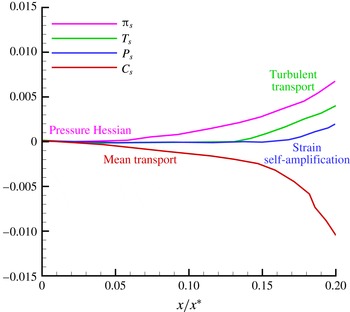
. It is of interest to magnify this region to see what really contributes to the generation of small-scale strain where there is no vorticity. A magnified view of figure 10(b) for
 $x/x^{\ast }<0.2$
is shown in figure 11. The first term to become active along the grid-element centreline is the strain pressure Hessian. This term is balanced by nothing else than the convection due to mean flow for
 $x/x^{\ast }<0.14$
. The pressure Hessian acts on the fluid elements to produce strain in the region where enstrophy is absent. It is clearly a non-local effect. Therefore, the mean strain-product equation for
 $x/x^{\ast }<0.14$
can be simplified as,
 $$\begin{eqnarray}\displaystyle U_{k}\frac{\unicode[STIX]{x2202}}{\unicode[STIX]{x2202}x_{k}}\left(\frac{1}{2}\langle \unicode[STIX]{x1D634}_{ij}\unicode[STIX]{x1D634}_{ij}\rangle \right)\approx -\left\langle \unicode[STIX]{x1D634}_{ij}\frac{\unicode[STIX]{x2202}^{2}p}{\unicode[STIX]{x2202}x_{i}\unicode[STIX]{x2202}x_{j}}\right\rangle . & & \displaystyle\end{eqnarray}$$
The importance of the pressure Hessian term in the vicinity of the grid-element was observed by Zhou et al. (Reference Zhou, Nagata, Sakai, Ito and Hayase2015) when the conditional mean trajectories of the
 $Q$
,
 $R$
invariants in the
 $Q{-}R$
plane were computed. It was not however directly identified as the dominant generating mechanism for strain in the lee of the grid-element, as we show in the present paper.
Once strain is produced by pressure Hessian, it is then transported by fluctuations as can be seen from figure 11, where the
 $T_{s}$
term becomes active after
 $x/x^{\ast }\approx 0.14$
, acting to increase
 $\langle \unicode[STIX]{x1D634}_{ij}\unicode[STIX]{x1D634}_{ij}\rangle$
. This transport, however, is not due to the lateral fluctuations, but due to the streamwise fluctuations which are generated by the pressure work mechanism, as discussed in § 5.1.1. The increase of small-scale strain leads to turning on of the strain self-amplification which starts being very significant from
 $x/x^{\ast }\approx 0.2$
. Therefore, equation (5.7) can be simplified for
 $0.14<x/x^{\ast }<0.2$
as,
 $$\begin{eqnarray}\displaystyle U_{k}\frac{\unicode[STIX]{x2202}}{\unicode[STIX]{x2202}x_{k}}\left(\frac{1}{2}\langle \unicode[STIX]{x1D634}_{ij}\unicode[STIX]{x1D634}_{ij}\rangle \right)\approx -\frac{1}{2}\frac{\unicode[STIX]{x2202}}{\unicode[STIX]{x2202}x_{k}}\langle u_{k}\unicode[STIX]{x1D634}_{ij}\unicode[STIX]{x1D634}_{ij}\rangle -\langle \unicode[STIX]{x1D634}_{ij}\unicode[STIX]{x1D634}_{jk}\unicode[STIX]{x1D634}_{ki}\rangle -\left\langle \unicode[STIX]{x1D634}_{ij}\frac{\unicode[STIX]{x2202}^{2}p}{\unicode[STIX]{x2202}x_{i}\unicode[STIX]{x2202}x_{j}}\right\rangle . & & \displaystyle\end{eqnarray}$$
Looking now at figure 10(b), the strain pressure Hessian term eventually becomes a sink after
 $x/x^{\ast }\approx 0.25$
. Around that location, enstrophy has been brought towards the grid-element centreline as discussed earlier and the presence of small-scale strain brought about by the dynamics in (5.8) and (5.9) initiates the vortex stretching term as seen in figures 10(b) and 8(b). From then on, vortex stretching and dissipation by viscosity become sinks of
 $\langle \unicode[STIX]{x1D634}_{ij}\unicode[STIX]{x1D634}_{ij}\rangle$
. Therefore, for
 $0.25<x/x^{\ast }<0.5$
, the transport of mean strain product is due to transport by fluctuations and strain self-amplification which are balanced by the sum of strain pressure Hessian, dissipation by viscosity, vortex stretching and convection due to mean flow. This can be written in equation form as,
 $$\begin{eqnarray}\displaystyle U_{k}\frac{\unicode[STIX]{x2202}}{\unicode[STIX]{x2202}x_{k}}\left(\frac{1}{2}\langle \unicode[STIX]{x1D634}_{ij}\unicode[STIX]{x1D634}_{ij}\rangle \right) & {\approx} & \displaystyle -\frac{1}{2}\frac{\unicode[STIX]{x2202}}{\unicode[STIX]{x2202}x_{k}}\langle u_{k}\unicode[STIX]{x1D634}_{ij}\unicode[STIX]{x1D634}_{ij}\rangle -\langle \unicode[STIX]{x1D634}_{ij}\unicode[STIX]{x1D634}_{jk}\unicode[STIX]{x1D634}_{ki}\rangle -\frac{1}{4}\langle \unicode[STIX]{x1D714}_{i}\unicode[STIX]{x1D714}_{j}\unicode[STIX]{x1D634}_{ij}\rangle \nonumber\\ \displaystyle & & \displaystyle -\left\langle \unicode[STIX]{x1D634}_{ij}\frac{\unicode[STIX]{x2202}^{2}p}{\unicode[STIX]{x2202}x_{i}\unicode[STIX]{x2202}x_{j}}\right\rangle +\unicode[STIX]{x1D708}\langle \unicode[STIX]{x1D634}_{ij}\unicode[STIX]{x1D6FB}^{2}\unicode[STIX]{x1D634}_{ij}\rangle .\end{eqnarray}$$
This analysis of mean strain product suggests that there are two subzones in the production region. One is the ‘strain-dominant’ zone where only strain is effectively present, and the other one is located adjacent to it further downstream where both strain and vorticity coexist.
In the decay region, the pressure Hessian term becomes zero and transport due to fluctuations becomes a homogenising consuming term. The mean convection term and the strain self-amplification term are balanced by enstrophy production (stretching), transport by fluctuations and dissipation. Therefore, the transport equation of mean strain product in the decay region can be written as,
 $$\begin{eqnarray}\displaystyle U_{k}\frac{\unicode[STIX]{x2202}}{\unicode[STIX]{x2202}x_{k}}\left(\frac{1}{2}\langle \unicode[STIX]{x1D634}_{ij}\unicode[STIX]{x1D634}_{ij}\rangle \right)\approx -\frac{1}{2}\frac{\unicode[STIX]{x2202}}{\unicode[STIX]{x2202}x_{k}}\langle u_{k}\unicode[STIX]{x1D634}_{ij}\unicode[STIX]{x1D634}_{ij}\rangle -\langle \unicode[STIX]{x1D634}_{ij}\unicode[STIX]{x1D634}_{jk}\unicode[STIX]{x1D634}_{ki}\rangle -\frac{1}{4}\langle \unicode[STIX]{x1D714}_{i}\unicode[STIX]{x1D714}_{j}\unicode[STIX]{x1D634}_{ij}\rangle +\unicode[STIX]{x1D708}\langle \unicode[STIX]{x1D634}_{ij}\unicode[STIX]{x1D6FB}^{2}\unicode[STIX]{x1D634}_{ij}\rangle . & & \displaystyle\end{eqnarray}$$
The mean velocity gradient terms such as
 $\unicode[STIX]{x1D6FC}_{s}$
,
 $\unicode[STIX]{x1D6FD}_{s}$
and
 $\unicode[STIX]{x1D708}_{s}$
do not contribute to the transport of mean strain product even in the inhomogeneous production region. The same was observed in the transport equation for enstrophy.
(a) Evolution of mean strain product along the bar centreline. (b) Budget of mean strain product along the bar centreline (all terms are normalised by
 $(U_{\infty }/t_{0})^{3}$
).

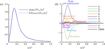
Unlike the grid-element centreline, strain and vorticity coexist throughout the bar centreline (see figure 12 a). The dynamics of the strain product and its budget along the bar centreline, as shown in figure 12(b), is similar to that of the bar centreline mean enstrophy discussed in the previous section. Here also, the turbulent stretching of fluctuating strain is the most dominant term, while the gradient production and stretching by mean strain rate contribute only marginally to the production of mean strain product. Compared to the enstrophy budget, the only difference is the presence of the strain pressure Hessian correlation term that acts as a source in a near-bar region, and eventually becomes a sink further downstream. Far downstream, strain self-amplification is balanced by viscous dissipation.
Here also, the balancing of budgets in the mean strain product is not perfect, yet the percentage error is minimal which makes these results acceptable. We repeat that this is the first time that such numerically well-balanced equations are presented in a study of this kind.
We close this subsection by discussing the effect of aspect ratio AR on the near field. As mentioned in § 2, the AR of the examined grid-element is 0.14, while in classical grids it is equal to 1. It is intuitive to expect that the AR of the bar will influence the near field, both in terms of size of the production region as well as the maximum r.m.s. velocity in the wake. To estimate the size of the production region, we can employ a similarity argument. Gomes-Fernandes et al. (Reference Gomes-Fernandes, Ganapathisubramani and Vassilicos2012) defined a modified wake-interaction length scale, denoted as
 ${x^{\ast }}^{\prime }$
, that was found to collapse the spatial variation of the normalised turbulent intensities for various grids. The definition of
 ${x^{\ast }}^{\prime }$
uses the drag coefficient (
 $C_{D}$
) of the bar, which is sensitive to AR. Bearman & Trueman (Reference Bearman and Trueman1972) measured the
 $C_{D}$
values of rectangular cylinders of different AR values.
 $C_{D}$
increases with AR, reaches a maximum value of 3 around
 $AR\approx 0.6$
, and then is reduced. This trend is found to be true also for low Reynolds number transitional flows (refer to Norberg Reference Norberg1993). Interestingly, for
 $AR=1.0$
and 0.14, the
 $C_{D}$
values are found to be very similar,
 $C_{D}\approx 2$
. Consequently, the modified wake-interaction length scale
 ${x^{\ast }}^{\prime }$
of the classical grid-element with
 $AR=1.0$
will be very close to one for the current grid-element. Based on this similarity argument, we expect the size of the production region for the two ARs to be close to each other. To the best of our knowledge, there are no similarity variables to predict the maximum r.m.s. values. Therefore one needs to perform additional simulations in order to confirm the prediction of the above similarity argument for the size of the production region as well as to compute the maximum turbulent intensity.
5.2 Energy spectra
Having understood the mechanism whereby the small-scale terms of turbulence are generated in this developing flow, this section investigates the relation between the small-scale terms and the energy spectra along the grid-element centreline.
Gomes-Fernandes, Ganapathisubramani & Vassilicos (Reference Gomes-Fernandes, Ganapathisubramani and Vassilicos2015) and Laizet et al. (Reference Laizet, Nedić and Vassilicos2015b
) obtained the energy spectra for turbulence generated by a fractal grid. Both studies confirmed that the
 $-5/3$
power-law slope exists for the energy spectrum, even in the production region where the turbulence is only developing, non-Gaussian and inhomogeneous. In fact, Laizet et al. (Reference Laizet, Nedić and Vassilicos2015b
) noted that, on the centreline, the
 $-5/3$
power law first appears half-way between
 $x=0$
and the turbulence peak. The DNS results of Laizet et al. (Reference Laizet, Vassilicos and Cambon2013) for fractal grid turbulence and of Zhou et al. (Reference Zhou, Nagata, Sakai, Ito and Hayase2016b
) for a single square grid-element turbulence confirm this finding on the
 $2/3$
power-law exponent of the second-order structure function. Clearly, this power-law behaviour in the energy spectrum is not related to the Kolmogorov theory (Kolmogorov Reference Kolmogorov1941) as none of the assumptions made in the Kolmogorov theory is valid in this region.
Energy spectra at different locations along the grid-element centreline: (a)
 $x/x^{\ast }=0.1$
, (b)
 $x/x^{\ast }=0.25$
, (c)
 $x/x^{\ast }=0.35$
, (d)
 $x/x^{\ast }=0.5$
, (e)
 $x/x^{\ast }=0.75$
, (f)
 $x/x^{\ast }=0.95$
. The frequencies
 $f$
have been normalised with the ratio of the free-stream velocity
 $U_{\infty }$
and the thickness
 $t_{0}$
.

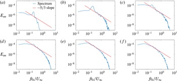
Figure 13 depicts the energy spectra obtained at all locations considered in the present study. Very close to the grid-element, where the flow is irrotational, the energy spectrum shows a pronounced vortex shedding signature with a normalised frequency (Strouhal number)
 $ft_{0}/U_{\infty }=0.21$
(figure 13
a). It is interesting that this shedding frequency is already found at a location in the grid-element centreline where the wakes have not yet met and the flow is irrotational. This indicates that it is probably the result of a global three-dimensional instability of the flow. As can be seen in figure 13(a), the energy content of this frequency is low (as expected since this point is not directly immersed in the wake) and there is no power law with a
 $-5/3$
slope. On the other hand, as depicted in figure 13(b), a power law in the energy spectrum with slope close to
 $-5/3$
is first observed at
 $x/x^{\ast }=0.25$
, for at least half a decade of frequency. The point
 $x/x^{\ast }=0.25$
is exactly half-way between
 $x=0$
and the turbulence peak which is where Gomes-Fernandes et al. (Reference Gomes-Fernandes, Ganapathisubramani and Vassilicos2015), Laizet et al. (Reference Laizet, Nedić and Vassilicos2015b
) found the best
 $-5/3$
power-law slope defined for a wide range of frequency. From the previous section, it is known that
 $x/x^{\ast }=0.25$
is the location where the turbulence is developing and inhomogeneous. The limited frequency range of
 $-5/3$
in our spectrum is consistent with the fact that the Reynolds number is particularly low. In fact, the local
 $Re_{\unicode[STIX]{x1D706}}$
is only 22.01 at
 $x/x^{\ast }=0.25$
(see table 1) and it can be surprising that a
 $-5/3$
power law exists at all, even in such a narrow frequency range. This result is in agreement with the observations made by Gomes-Fernandes et al. (Reference Gomes-Fernandes, Ganapathisubramani and Vassilicos2015), Laizet et al. (Reference Laizet, Nedić and Vassilicos2015b
) albeit at much higher Reynolds numbers, which explains why their
 $-5/3$
power law at a location midway between the grid-element and turbulence peak was defined over at least one decade of frequency.
The energy spectra in the further downstream locations of the developing region (i.e.
 $x/x^{\ast }<0.5$
) also exhibit a restricted
 $-5/3$
power law and a less pronounced vortex shedding signature as seen in figure 13(c,d). However, the
 $-5/3$
slope is progressively eroded in these locations (see figure 13
c,d) compared to the spectra at
 $x/x^{\ast }=0.25$
(figure 13
b). The erosion of the
 $2/3$
power law from the near field to the downstream in the second-order structure function, directly related to the
 $-5/3$
law of the spectra, was also observed by Zhou et al. (Reference Zhou, Nagata, Sakai, Ito and Hayase2016b
). It should be reminded that the Kolmogorov theory is not applicable in this developing turbulence region.
The energy spectra at the fully developed turbulent region are represented in figures 13(e) and 13(f). At these locations, the Kolmogorov theory is applicable as flow in the region of
 $x/x^{\ast }>0.5$
is fully turbulent and homogeneous (refer to § 5.1). Note that the local
 $Re_{\unicode[STIX]{x1D706}}$
of this region is considerably higher than that of
 $x/x^{\ast }=0.25$
(see table 1). Yet, the frequency range of
 $-5/3$
power-law slope is shorter compared to the frequency range observed at
 $x/x^{\ast }=0.25$
.
The energy spectrum in figure 13(b) appears to acquire a shape which includes a short range reminiscent of a
 $-5/3$
power law at the start of the subregion where (5.10) holds and where strain self-amplification and vortex stretching have only just started being both significantly present. This is also the subregion where the pressure Hessian acts like a sink. The spectral range which is emulating a short
 $-5/3$
power law does not grow but in fact diminishes as vortex stretching and strain self-amplification increase to their maximum values at
 $x=0.5x^{\ast }$
and this range continues to diminish further downstream in the decay region. These conclusions echo those of Laizet et al. (Reference Laizet, Vassilicos and Cambon2013), Gomes-Fernandes et al. (Reference Gomes-Fernandes, Ganapathisubramani and Vassilicos2015) and Laizet et al. (Reference Laizet, Nedić and Vassilicos2015b
) who obtained energy spectra at much higher Reynolds numbers but were not able to have as much concurrent detail on the small-scale strain and vorticity dynamics as we have here.
5.3 Enstrophy production and strain self-amplification
Having identified the mechanism whereby small-scale strain rate and vorticity fluctuations are amplified, as well as their association with the energy spectra, we now turn our attention to the statistical study of two of the most important velocity gradient terms which contribute to the generation of mean enstrophy and strain product along the grid-element centreline: mean enstrophy production
 $\langle \unicode[STIX]{x1D714}_{i}\unicode[STIX]{x1D714}_{j}\unicode[STIX]{x1D634}_{ij}\rangle$
and mean strain self-amplification
 $\langle \unicode[STIX]{x1D634}_{ij}\unicode[STIX]{x1D634}_{jk}\unicode[STIX]{x1D634}_{ki}\rangle$
. We discuss their statistics in this subsection.
Values of normalised
 $\langle \unicode[STIX]{x1D714}_{i}\unicode[STIX]{x1D714}_{j}\unicode[STIX]{x1D634}_{ij}\rangle$
,
 $\langle \unicode[STIX]{x1D634}_{ij}\unicode[STIX]{x1D634}_{jk}\unicode[STIX]{x1D634}_{ki}\rangle$
and their ratios at different stations along the grid-element centreline. The values of field experiment are taken from Gulitski et al. (Reference Gulitski, Kholmyansky, Kinzelbach, Lüthi, Tsinober and Yorish2007) and the grid experiment is taken from the decay region of Gomes-Fernandes et al. (Reference Gomes-Fernandes, Ganapathisubramani and Vassilicos2014).

It was already shown in figures 8(a) and 10(a) that the mean enstrophy production and strain self-amplification increase in the production region, and then in the decay region their values decrease. Table 2 records the values of these quantities normalised by
 $\langle \unicode[STIX]{x1D634}_{ij}\unicode[STIX]{x1D634}_{ij}\rangle ^{3/2}$
. The normalised values of
 $\langle \unicode[STIX]{x1D714}_{i}\unicode[STIX]{x1D714}_{j}\unicode[STIX]{x1D634}_{ij}\rangle$
and
 $\langle \unicode[STIX]{x1D634}_{ij}\unicode[STIX]{x1D634}_{jk}\unicode[STIX]{x1D634}_{ki}\rangle$
decrease from the turbulence peak onwards. These quantities are compared against the reference values taken from the grid and field experiments. It can be seen that the normalised values decay in the region
 $x/x^{\ast }\geqslant 0.5$
allowing for the possibility that they might tend towards values comparable to the reference values given in the table. However, there is of course no guarantee that this is indeed so, and our simulation is not long enough in the streamwise direction for us to check. The ratio of
 $\langle -\unicode[STIX]{x1D714}_{i}\unicode[STIX]{x1D714}_{j}\unicode[STIX]{x1D634}_{ij}\rangle /\langle \unicode[STIX]{x1D634}_{ij}\unicode[STIX]{x1D634}_{jk}\unicode[STIX]{x1D634}_{ki}\rangle$
is also given in the table and compared with the reference value taken from the classical grid experiment. The reference value is close to the ratio
 $4/3(=1.33)$
for homogeneous turbulence (Tsinober Reference Tsinober2009). The value of
 $(4/3)$
is also closely predicted by our simulations at the downstream end of the computational domain. Besides, the variation of
 $\langle -\unicode[STIX]{x1D714}_{i}\unicode[STIX]{x1D714}_{j}\unicode[STIX]{x1D634}_{ij}\rangle /\langle \unicode[STIX]{x1D634}_{ij}\unicode[STIX]{x1D634}_{jk}\unicode[STIX]{x1D634}_{ki}\rangle$
in our simulation qualitatively agrees with the low blockage grid-element simulations of Zhou et al. (Reference Zhou, Nagata, Sakai, Ito and Hayase2016a
).
Comparison of the normalised enstrophy production and self-amplification values with the values reported by Gomes-Fernandes et al. (Reference Gomes-Fernandes, Ganapathisubramani and Vassilicos2014) (table 6 in their paper) reveals some differences. In their study, the ratios of
 $\langle \unicode[STIX]{x1D714}_{i}\unicode[STIX]{x1D714}_{j}\unicode[STIX]{x1D634}_{ij}\rangle$
and
 $\langle \unicode[STIX]{x1D634}_{ij}\unicode[STIX]{x1D634}_{jk}\unicode[STIX]{x1D634}_{ki}\rangle$
to
 $\langle \unicode[STIX]{x1D634}_{ij}\unicode[STIX]{x1D634}_{ij}\rangle ^{3/2}$
are 12 % and 10 % respectively in the middle of the production region and then they increase to 21 % and 26 % in the decay region. In the present study, however, these ratios are much larger, as can be seen from table 2. The reason for this difference is that the denominator
 $\langle \unicode[STIX]{x1D634}_{ij}\unicode[STIX]{x1D634}_{ij}\rangle ^{3/2}$
is small in our production region, but increases very rapidly further downstream as shown in figure 10(a). In fact, it increases by a factor of 7 from the middle of the production region to the peak. On the other hand in figure 10 of Gomes-Fernandes et al. (Reference Gomes-Fernandes, Ganapathisubramani and Vassilicos2014),
 $\langle \unicode[STIX]{x1D634}_{ij}\unicode[STIX]{x1D634}_{ij}\rangle$
increases by approximately a factor of 2 only. This suggests that the fractal grid produces a more homogeneous strain field compared to the single square grid-element. This may not be only due to the multi-scale space filling properties of the grid (i.e. the presence of bars of different sizes that homogenise the flow), but also to the fact that their incoming flow carries significant turbulence intensity, and therefore strain.
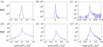
Probability density function (PDF) of enstrophy production at different locations along the grid-element centreline: (a)
 $x/x^{\ast }=0.1$
, (b)
 $x/x^{\ast }=0.25$
, (c)
 $x/x^{\ast }=0.35$
, (d)
 $x/x^{\ast }=0.5$
, (e)
 $x/x^{\ast }=0.75$
, (f)
 $x/x^{\ast }=0.95$
.

It is interesting to note that at
 $x/x^{\ast }=0.25$
, where the wakes have already met, the turbulence is developing and the energy spectrum has a
 $-5/3$
power-law slope (from our simulation but perhaps more importantly from the higher Reynolds number measurements and simulations of Laizet et al. (Reference Laizet, Vassilicos and Cambon2013), Gomes-Fernandes et al. (Reference Gomes-Fernandes, Ganapathisubramani and Vassilicos2015) and Laizet et al. (Reference Laizet, Nedić and Vassilicos2015b
)), the mean strain self-amplification dominates the mean enstrophy production at least by a factor of two. This observation correlates the emergence of
 $-5/3$
energy spectra with the dominance of strain self-amplification process rather than of vortex stretching. Downstream of
 $x/x^{\ast }=0.25$
, the mean enstrophy production soon dominates over mean strain self-amplification, but the
 $-5/3$
slope in the energy spectrum gradually weakens. It seems that the strain self-amplification is more essential for the energy spectrum’s
 $-5/3$
power-law shape than vortex stretching even though
 $\langle \unicode[STIX]{x1D714}_{i}\unicode[STIX]{x1D714}_{j}\unicode[STIX]{x1D634}_{ij}\rangle >0$
(as is in fact the case) signifies prevalence of vortex stretching over vortex compression.
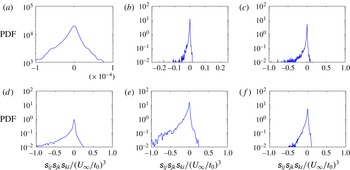
PDF of strain self-amplification at different locations along the grid-element centreline: (a)
 $x/x^{\ast }=0.1$
, (b)
 $x/x^{\ast }=0.25$
, (c)
 $x/x^{\ast }=0.35$
, (d)
 $x/x^{\ast }=0.5$
, (e)
 $x/x^{\ast }=0.75$
, (f)
 $x/x^{\ast }=0.95$
.

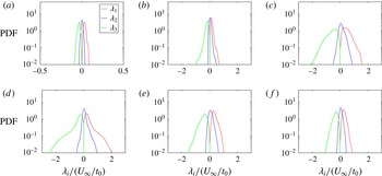
The PDFs of enstrophy production are shown in figure 14 for all the locations considered in this study. The PDF looks almost symmetric in the irrotational flow grid-element centreline region with the negligible values of
 $\unicode[STIX]{x1D714}_{i}\unicode[STIX]{x1D634}_{ij}\unicode[STIX]{x1D714}_{j}$
(figure 14
a). At
 $x/x^{\ast }=0.25$
, where the slope in the energy spectrum is first observed to be
 $-5/3$
, the PDF of
 $\unicode[STIX]{x1D714}_{i}\unicode[STIX]{x1D634}_{ij}\unicode[STIX]{x1D714}_{j}$
is clearly skewed towards positive, as seen in figure 14(b). This indicates that vortex stretching is preferred over vortex compression at the onset point of
 $-5/3$
slope in the energy spectrum where the turbulence is still developing and inhomogeneous. This is an interesting result as the experimental study of fractal grid turbulence by Gomes-Fernandes et al. (Reference Gomes-Fernandes, Ganapathisubramani and Vassilicos2014) reported that the tendency for vortex stretching dominance is not evident in the inhomogeneous production region of fractal grid (see § 4.2 on p. 268 of Gomes-Fernandes et al. (Reference Gomes-Fernandes, Ganapathisubramani and Vassilicos2014)). A plausible reason for this discrepancy is discussed in § 5.5.2 with the help of the intermediate strain-rate eigenvalue
 $\unicode[STIX]{x1D706}_{2}$
. In all other locations beyond
 $x/x^{\ast }=0.25$
, the PDF of
 $\unicode[STIX]{x1D714}_{i}\unicode[STIX]{x1D634}_{ij}\unicode[STIX]{x1D714}_{j}$
is skewed towards positive, signifying the prevalence of vortex stretching over vortex compression, which is a universal characteristic of small scales in turbulent flows (Taylor Reference Taylor1938; Betchov Reference Betchov1975; Tsinober, Kit & Dracos Reference Tsinober, Kit and Dracos1992; Tsinober et al.
Reference Tsinober, Shtilman, Sinyavskii and Vaisburd1995). It is interesting that this universal result is obtained for
 $Re_{\unicode[STIX]{x1D706}}$
as low as 33 in our decay region where the turbulence is fully developed and homogeneous. Although we notice differences in the near-grid-element PDF of
 $\unicode[STIX]{x1D714}_{i}\unicode[STIX]{x1D634}_{ij}\unicode[STIX]{x1D714}_{j}$
when compared against the experimental result of Gomes-Fernandes et al. (Reference Gomes-Fernandes, Ganapathisubramani and Vassilicos2014), our results agree with the DNS result of Zhou et al. (Reference Zhou, Nagata, Sakai, Ito and Hayase2016a
).
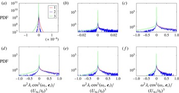
The PDFs of strain self-amplification are depicted in figure 15. At the irrotational flow grid-element centreline, the PDF of
 $\unicode[STIX]{x1D634}_{ij}\unicode[STIX]{x1D634}_{jk}\unicode[STIX]{x1D634}_{ki}$
is nearly symmetric with very small values of
 $\unicode[STIX]{x1D634}_{ij}\unicode[STIX]{x1D634}_{jk}\unicode[STIX]{x1D634}_{ki}$
(figure 15
a). From figure 15(b–f), it can be observed that the PDFs are skewed towards a negative average in the regions where the wakes have met, which is also considered to be a universal characteristic of turbulent flows (Tsinober Reference Tsinober2000, Reference Tsinober2009). Again the universal statistical behaviour of strain self-amplification is noted for very low
 $Re_{\unicode[STIX]{x1D706}}$
values of homogeneous fully developed turbulence (see figures 15
e and 15
f). Gomes-Fernandes et al. (Reference Gomes-Fernandes, Ganapathisubramani and Vassilicos2014) and Zhou et al. (Reference Zhou, Nagata, Sakai, Ito and Hayase2016a
) also reported negative average values of strain self-amplification in the production region.
5.4 Invariants of the velocity gradient tensor
The next objective is to test the validity of other potentially universal characteristics of the invariants of VGT for the low Reynolds number turbulence considered here. A brief review of equations and terms used in this study is given first, followed by the analysis of the JPDF of the VGT invariants.
The VGT
 $\unicode[STIX]{x1D608}_{ij}=\unicode[STIX]{x2202}u_{i}/\unicode[STIX]{x2202}x_{j}$
can be decomposed into symmetric and antisymmetric parts. The symmetric part is the strain-rate tensor
 $\unicode[STIX]{x1D634}_{ij}$
, and the antisymmetric part is the rotation-rate tensor
 $\unicode[STIX]{x1D6FA}_{ij}$
(which can be written in terms of vorticity components
 $\unicode[STIX]{x1D714}_{k}$
as
 $\unicode[STIX]{x1D6FA}_{ij}=-\unicode[STIX]{x1D716}_{ijk}\unicode[STIX]{x1D714}_{k}/2$
). The characteristic equation of the velocity gradient tensor is,
 $$\begin{eqnarray}\displaystyle \unicode[STIX]{x1D6EC}_{i}^{3}+P\unicode[STIX]{x1D6EC}_{i}^{2}+Q\unicode[STIX]{x1D6EC}_{i}+R=0, & & \displaystyle\end{eqnarray}$$
where
 $\unicode[STIX]{x1D6EC}_{i}$
(
 $i=1,2,3$
) are the three eigenvalues and
 $P$
,
 $Q$
,
 $R$
are the first, second and third invariants respectively. For incompressible flow, the first invariant is zero (
 $P=0$
). The second and third invariants are,
 $$\begin{eqnarray}\displaystyle & \displaystyle Q={\textstyle \frac{1}{4}}(\unicode[STIX]{x1D714}_{i}\unicode[STIX]{x1D714}_{i}-2\unicode[STIX]{x1D634}_{ij}\unicode[STIX]{x1D634}_{ij}), & \displaystyle\end{eqnarray}$$
 $$\begin{eqnarray}\displaystyle & \displaystyle R=-{\textstyle \frac{1}{3}}\left(\unicode[STIX]{x1D634}_{ij}\unicode[STIX]{x1D634}_{jk}\unicode[STIX]{x1D634}_{ki}+{\textstyle \frac{3}{4}}\unicode[STIX]{x1D714}_{i}\unicode[STIX]{x1D714}_{j}\unicode[STIX]{x1D634}_{ij}\right). & \displaystyle\end{eqnarray}$$
The discriminant of the cubic equation (5.12) is
 $$\begin{eqnarray}\displaystyle D={\textstyle \frac{27}{4}}R^{2}+Q^{3} & & \displaystyle\end{eqnarray}$$
and if it is negative, all three eigenvalues are real and distinct. The invariants of the strain-rate tensor are obtained by setting
 $\unicode[STIX]{x1D714}_{i}=0$
in (5.13) and (5.14), and they are
 $$\begin{eqnarray}\displaystyle & \displaystyle Q_{s}=-{\textstyle \frac{1}{2}}\unicode[STIX]{x1D634}_{ij}\unicode[STIX]{x1D634}_{ij}, & \displaystyle\end{eqnarray}$$
 $$\begin{eqnarray}\displaystyle & \displaystyle R_{s}=-{\textstyle \frac{1}{3}}\unicode[STIX]{x1D634}_{ij}\unicode[STIX]{x1D634}_{jk}\unicode[STIX]{x1D634}_{ki}. & \displaystyle\end{eqnarray}$$
Finally, the single invariant of the rotation-rate tensor is acquired by putting
 $\unicode[STIX]{x1D634}_{ij}=0$
in (5.13), and it is,
 $$\begin{eqnarray}\displaystyle & \displaystyle Q_{w}={\textstyle \frac{1}{4}}\unicode[STIX]{x1D714}_{i}\unicode[STIX]{x1D714}_{i}. & \displaystyle\end{eqnarray}$$
The study of invariants of the velocity gradient, strain-rate and rotation-rate tensors often reveal information regarding the local topology of the flow field. Furthermore, they also contain information regarding vortex stretching and rotation. They have been studied extensively for various turbulent flows.
Laizet et al. (Reference Laizet, Vassilicos and Cambon2013) were the first to analyse the spatial evolution of
 $Q{-}R$
diagrams in a spatially evolving turbulent flow behind a fractal grid. They found that these diagrams obtain their usual teardrop shape well downstream of the point where the second-order structure function acquires its
 $2/3$
power law in the production region. Gomes-Fernandes et al. (Reference Gomes-Fernandes, Ganapathisubramani and Vassilicos2014) reported from their particle image velocimetry (PIV) study that the
 $Q{-}R$
diagram clearly gets its usual shape only in the decay region. Zhou et al. (Reference Zhou, Nagata, Sakai, Ito and Hayase2016b
) also presented
 $Q{-}R$
diagrams in the production region of a single square grid-element and confirmed that they are qualitatively different from the well-known teardrop shape which appears in the decay region. Information on the
 $Q_{s}{-}R_{s}$
diagram for a single square grid-element turbulence is still missing.
5.4.1
 $Q$
–
$R$
diagrams


In this section we study the joint PDFs of
 $Q{-}R$
, i.e.
 $Q{-}R$
diagrams. To interpret
 $Q{-}R$
diagrams, one needs to rewrite (5.14) as
 $3R=-\unicode[STIX]{x1D634}_{ij}\unicode[STIX]{x1D634}_{jk}\unicode[STIX]{x1D634}_{ki}-\unicode[STIX]{x1D714}_{i}\unicode[STIX]{x1D714}_{j}\unicode[STIX]{x1D634}_{ij}/4-\unicode[STIX]{x1D714}_{i}\unicode[STIX]{x1D714}_{j}\unicode[STIX]{x1D634}_{ij}/2$
. This reveals that
 $3R$
is the difference between two production terms: the term
 $-\unicode[STIX]{x1D634}_{ij}\unicode[STIX]{x1D634}_{jk}\unicode[STIX]{x1D634}_{ki}-\unicode[STIX]{x1D714}_{i}\unicode[STIX]{x1D714}_{j}\unicode[STIX]{x1D634}_{ij}/4$
(the average of which appears in the equation for
 $\langle \unicode[STIX]{x1D634}_{ij}\unicode[STIX]{x1D634}_{ij}\rangle /2$
, equation (5.7)) and the term
 $\unicode[STIX]{x1D714}_{i}\unicode[STIX]{x1D714}_{j}\unicode[STIX]{x1D634}_{ij}/2$
(the average of which appears in the equation for
 $\langle \unicode[STIX]{x1D714}_{i}\unicode[STIX]{x1D714}_{i}\rangle /4$
, i.e. (5.4) multiplied by
 $1/2$
on both sides). The reason for considering the production of
 $\unicode[STIX]{x1D714}_{i}\unicode[STIX]{x1D714}_{i}/4$
rather than
 $\unicode[STIX]{x1D714}_{i}\unicode[STIX]{x1D714}_{i}/2$
lies in the fact that
 $Q=\unicode[STIX]{x1D714}_{i}\unicode[STIX]{x1D714}_{i}/4-\unicode[STIX]{x1D634}_{ij}\unicode[STIX]{x1D634}_{ij}/2$
. Hence in a
 $Q$
–
 $R$
plot, the upper left quadrant (where
 $Q>0$
and
 $R<0$
) represents events in which
 $\unicode[STIX]{x1D714}_{i}\unicode[STIX]{x1D714}_{i}/4$
dominates over
 $\unicode[STIX]{x1D634}_{ij}\unicode[STIX]{x1D634}_{ij}/2$
and the production of
 $\unicode[STIX]{x1D714}_{i}\unicode[STIX]{x1D714}_{i}/4$
also dominates over the production of
 $\unicode[STIX]{x1D634}_{ij}\unicode[STIX]{x1D634}_{ij}/2$
. In the upper right quadrant (where
 $Q>0$
and
 $R>0$
)
 $\unicode[STIX]{x1D714}_{i}\unicode[STIX]{x1D714}_{i}/4$
dominates over
 $\unicode[STIX]{x1D634}_{ij}\unicode[STIX]{x1D634}_{ij}/2$
but the production of
 $\unicode[STIX]{x1D634}_{ij}\unicode[STIX]{x1D634}_{ij}/2$
dominates over the production of
 $\unicode[STIX]{x1D714}_{i}\unicode[STIX]{x1D714}_{i}/4$
. The lower left quadrant (where
 $Q<0$
and
 $R<0$
) represents events in which
 $\unicode[STIX]{x1D634}_{ij}\unicode[STIX]{x1D634}_{ij}/2$
dominates over
 $\unicode[STIX]{x1D714}_{i}\unicode[STIX]{x1D714}_{i}/4$
and where the production of
 $\unicode[STIX]{x1D634}_{ij}\unicode[STIX]{x1D634}_{ij}/2$
also dominates over the production of
 $\unicode[STIX]{x1D714}_{i}\unicode[STIX]{x1D714}_{i}/4$
; and finally, the lower right quadrant (where
 $Q<0$
and
 $R>0$
) includes events where
 $\unicode[STIX]{x1D634}_{ij}\unicode[STIX]{x1D634}_{ij}/2$
dominates over
 $\unicode[STIX]{x1D714}_{i}\unicode[STIX]{x1D714}_{i}/4$
, but the production of
 $\unicode[STIX]{x1D714}_{i}\unicode[STIX]{x1D714}_{i}/4$
dominates over the production of
 $\unicode[STIX]{x1D634}_{ij}\unicode[STIX]{x1D634}_{ij}/2$
. In many turbulent flows the
 $Q{-}R$
diagram has a teardrop shape (Chong, Perry & Cantwell Reference Chong, Perry and Cantwell1990; Tsinober Reference Tsinober2009). This shape reflects strong correlations between
 $Q<0$
and
 $R>0$
on one hand and between
 $Q>0$
and
 $R<0$
on the other.
Values of the normalised mean
 $\langle Q\rangle$
and
 $\langle R\rangle$
at different locations along the grid-element centreline.

The values of normalised
 $\langle Q\rangle$
and
 $\langle R\rangle$
are shown in table 3. It can be seen from the table that the values of
 $\langle Q\rangle$
are not zero in the region
 $x/x^{\ast }\leqslant 0.35$
, making it absolutely clear that this region is not homogeneous, even for small-scale statistics. The table shows that, on average, strain product dominates over enstrophy in this region as already seen in § 5.1. Strain is the first small-scale velocity gradient quantity generated along the grid-element centreline by the mechanism discussed in § 5.1. Note, however, that this strain dominance progressively disappears once vorticity is brought to the grid-element centreline. By the end of the production region, the average of both invariants is 0, which is the expected result for homogeneous turbulence.
Joint PDF of
 $Q$
and
 $R$
at different locations along the grid-element centreline: (a)
 $x/x^{\ast }=0.1$
, (b)
 $x/x^{\ast }=0.25$
, (c)
 $x/x^{\ast }=0.35$
, (d)
 $x/x^{\ast }=0.5$
, (e)
 $x/x^{\ast }=0.75$
, (f)
 $x/x^{\ast }=0.95$
. The isocontours range from
 $10^{1}$
to
 $10^{-2}$
.

Figure 16 shows the JPDF of
 $Q$
and
 $R$
at six different locations. The blue line in this figure is the locus of points where
 $D=0$
(5.15). The invariants are normalised by the mean strain product at that location. In the region where the wakes have not met and the flow is irrotational (
 $x/x^{\ast }=0.1$
), the shape of the
 $Q{-}R$
diagram is very different from the usual teardrop shape, and contains no positive
 $Q$
values (figure 16
a). This observation is consistent with and strengthens the previous observation that the flow in the initial part of the grid-element centreline is mostly irrotational, and
 $Q<0$
at all
 $x/x^{\ast }<0.2$
. In this region, the VGT is almost equal to the strain-rate tensor, which is a symmetric tensor, and therefore all the eigenvalues are real. This explains why all isolines are located below the
 $D=0$
curve, in an area where
 $D<0$
. The shape of JPDF at
 $x/x^{\ast }<0.1$
is similar to the one reported for the non-turbulent side of turbulent/non-turbulent interfaces (da Silva & Pereira Reference da Silva and Pereira2008). The shape of figure 16(a) also ascertains that the flow in the initial part of the grid-element centreline is indeed non-turbulent.
Although the wakes have already met by
 $x/x^{\ast }=0.25$
and the energy spectrum exhibits a short-range approximate
 $-5/3$
power-law exponent, the
 $Q{-}R$
diagram, as shown in figure 16(b), does not show its usual shape. However, it is interesting to note that
 $Q<0$
already correlates with
 $R>0$
with a visible tail in the
 $Q{-}R$
diagram at
 $x/x^{\ast }=0.25$
. This is also the point on the grid-element centreline where strain self-amplification and vortex stretching just started being significant, and the turbulence is still developing, non-Gaussian and inhomogeneous. The undeveloped shape in the
 $Q{-}R$
diagram in figure 16(b) for
 $x/x^{\ast }=0.25$
is due to the fact that the strain still dominates enstrophy. It should be noted that the undeveloped
 $Q{-}R$
diagram in the production region reported by Gomes-Fernandes et al. (Reference Gomes-Fernandes, Ganapathisubramani and Vassilicos2014) (see their figure 17a) correlates with an indistinguishable or slight dominance of vortex stretching over vortex compression while our results show a clear dominance of vortex stretching over compression.
From
 $x/x^{\ast }=0.35$
onwards the
 $Q{-}R$
diagrams evolve towards their usual teardrop shape as
 $Q$
starts to take both positive and negative values, and the correlation between
 $Q>0$
and
 $R<0$
starts to appear as seen in figure 16(c). This observation suggests that the preference for vortex stretching increases from the production to the decay region.
In this study, the
 $Q{-}R$
diagram is observed to attain its usual shape around
 $x/x^{\ast }=0.5$
i.e. at the end of the production region, as seen in figure 16(d). Our results agree with the numerical results of Laizet et al. (Reference Laizet, Vassilicos and Cambon2013) that the
 $Q{-}R$
diagram obtains its teardrop shape by the end of the production region and well downstream of the place where the
 $-5/3$
spectra and the
 $2/3$
structure functions first appear. Zhou et al. (Reference Zhou, Nagata, Sakai, Suzuki, Ito, Terashima and Hayase2014a
, Reference Zhou, Nagata, Sakai, Ito and Hayase2015) obtained the teardrop shape closer to the grid-element, at
 $x/x^{\ast }=0.16$
. This discrepancy could be due to the difference noticed in the behaviour of skewness and flatness which is the result of different blockage ratios in these two studies (0.11 as opposed to 0.2 in the present study). Also, this is the first study that reports the appearance of a teardrop shape in the
 $Q{-}R$
diagram for a very low
 $Re_{\unicode[STIX]{x1D706}}$
homogeneous fully developed turbulence (see figures 16
e and 16
f).
5.4.2
$Q_{s}{-}R_{s}$
diagrams and strain-rate eigenvalue ratios

We assume that the strain-rate eigenvalues are
 $\unicode[STIX]{x1D706}_{i}(i=1,2,3)$
with
 $\unicode[STIX]{x1D706}_{1}>\unicode[STIX]{x1D706}_{2}>\unicode[STIX]{x1D706}_{3}$
and
 $\unicode[STIX]{x1D706}_{1}+\unicode[STIX]{x1D706}_{2}+\unicode[STIX]{x1D706}_{3}=0$
for an incompressible flow. To interpret
 $Q_{s}{-}R_{s}$
diagrams, note that
 $R_{s}$
can be written in terms of
 $\unicode[STIX]{x1D706}_{i}$
as
 $R_{s}=-\unicode[STIX]{x1D706}_{1}\unicode[STIX]{x1D706}_{2}\unicode[STIX]{x1D706}_{3}$
. One might therefore expect some tendency for sheet-like vortex structures if
 $R_{s}>0$
(two extensive strain-rate eigenvalues) and some tendency for tube-like vortex structures if
 $R_{s}<0$
(two compressive strain-rate eigenvalues).
Defining
 $a=\unicode[STIX]{x1D706}_{2}/\unicode[STIX]{x1D706}_{1}$
, the following equation can be obtained:
 $$\begin{eqnarray}\displaystyle R_{s}=(-Q_{s})^{3/2}a(1+a)(1+a+a^{2})^{-3/2}. & & \displaystyle\end{eqnarray}$$
The flow geometry can be defined in terms of ratios of the eigenvalues of strain-rate tensor. The ratio
 $\unicode[STIX]{x1D706}_{1}\,\text{:}\,\unicode[STIX]{x1D706}_{2}\,\text{:}\,\unicode[STIX]{x1D706}_{3}=2\,\text{:}\,-1\,\text{:}\,-1$
(
 $a=-1/2$
) corresponds to axisymmetric contraction,
 $1\,\text{:}\,0\,\text{:}\,-1$
(
 $a=0$
) is for a two-dimensional flow,
 $3\,\text{:}\,1\,\text{:}\,-4$
(
 $a=1/3$
) represents biaxial stretching, and
 $1\,\text{:}\,1\,\text{:}\,-2$
(
 $a=1$
) is for axial stretching (da Silva & Pereira Reference da Silva and Pereira2008).
Joint PDF of
 $Q_{s}$
and
 $R_{s}$
at different locations along the grid-element centreline: (a)
 $x/x^{\ast }=0.1$
, (b)
 $x/x^{\ast }=0.25$
, (c)
 $x/x^{\ast }=0.35$
, (d)
 $x/x^{\ast }=0.5$
, (e)
 $x/x^{\ast }=0.75$
, (f)
 $x/x^{\ast }=0.95$
. The isocontours range from
 $10^{1}$
to
 $10^{-2}$
. The four lines from the left to the right in each panel correspond to
 $\unicode[STIX]{x1D706}_{1}\,\text{:}\,\unicode[STIX]{x1D706}_{2}\,\text{:}\,\unicode[STIX]{x1D706}_{3}=2\,\text{:}\,-1\,\text{:}\,-1$
,
 $1\,\text{:}\,0\,\text{:}\,-1$
,
 $3\,\text{:}\,1\,\text{:}\,-4$
and
 $1\,\text{:}\,1\,\text{:}\,-2$
.

Figure 17 shows the JPDF of
 $Q_{s}$
and
 $R_{s}$
in the production and decay regions. There is no real preference for positive or negative
 $R_{s}$
in the irrotational flow region as shown in figure 17(a). The contour lines align with the ratio of
 $1\,\text{:}\,0\,\text{:}\,-1$
at
 $x/x^{\ast }=0.1$
which shows that the irrotational flow is largely two-dimensional. From
 $x/x^{\ast }=0.25$
onwards the JPDF starts showing a tendency towards positive
 $R_{s}$
though the preference is very small at
 $x/x^{\ast }=0.25$
(figure 17
b). From
 $x/x^{\ast }=0.35$
onwards the JPDF looks similar to what is observed for homogeneous isotropic turbulence with larger probabilities occurring between
 $\unicode[STIX]{x1D706}_{1}\,\text{:}\,\unicode[STIX]{x1D706}_{2}\,\text{:}\,\unicode[STIX]{x1D706}_{3}=3\,\text{:}\,1\,\text{:}\,-4$
and
 $1\,\text{:}\,1\,\text{:}\,-2$
. Here also, the universal characteristics of
 $Q_{s}$
–
 $R_{s}$
diagram is obtained for a very low
 $Re_{\unicode[STIX]{x1D706}}$
homogeneous turbulence of our decay region (see figures 17
e and 17
f).
(a) Mean trajectory of
 $Q_{s}$
and
 $R_{s}$
in the phase map. Triangles represent the production region and circles the decay region. (b) Eigenvalue ratios
 $\unicode[STIX]{x1D706}_{1}\,\text{:}\,\unicode[STIX]{x1D706}_{2}\,\text{:}\,\unicode[STIX]{x1D706}_{3}$
along the grid-element centreline.

Figure 18 shows the trajectory of
 $\langle Q_{s}\rangle$
and
 $\langle R_{s}\rangle$
in their associated phase map. In figure 18(a), the triangles represent locations in the production region as one moves downstream along the grid-element centreline. The value of
 $\langle R_{s}\rangle$
grows from being negligibly small in the near-grid-element region to being slightly above
 $0.1\langle \unicode[STIX]{x1D634}_{ij}\unicode[STIX]{x1D634}_{ij}\rangle$
at
 $x/x^{\ast }\approx 0.4$
then dropping again as the turbulence peak location is approached. The circles represent locations in the decay region. This phase map can also be plotted in terms of
 $x/x^{\ast }$
as shown in figure 18(b). The first observation from these figures is that the average invariant values are in the quadrant of
 $Q_{s}<0$
and
 $R_{s}>0$
, and that they are mostly on the line
 $a=1$
for
 $0\leqslant x/x^{\ast }<0.4$
, and mostly on or near the line
 $a=1/3$
for the decay region. The transition between axial stretching to biaxial stretching occurs in the region of
 $0.4<x/x^{\ast }<0.5$
. The eigenvalue ratio in this transitional region is close to
 $2\,\text{:}\,1\,\text{:}\,-3$
. Note that the most probable eigenvalue ratios obtained in most previous studies are
 $3\,\text{:}\,1\,\text{:}\,-4$
and
 $2\,\text{:}\,1\,\text{:}\,-3$
(da Silva & Pereira Reference da Silva and Pereira2008).
5.5 Factors affecting enstrophy production and strain self-amplification
Finally in this subsection, we analyse the factors that affect the important velocity gradient terms. For an incompressible flow, the enstrophy production and strain self-amplification can be written in terms of the strain-rate eigenvalues, and the alignments between the vorticity vector and the strain-rate eigenvectors. More specifically:
 $$\begin{eqnarray}\displaystyle & \unicode[STIX]{x1D714}_{i}\unicode[STIX]{x1D714}_{j}\unicode[STIX]{x1D634}_{ij}=\unicode[STIX]{x1D714}^{2}\unicode[STIX]{x1D706}_{1}\cos ^{2}(\unicode[STIX]{x1D74E},\boldsymbol{e}_{\mathbf{1}})+\unicode[STIX]{x1D714}^{2}\unicode[STIX]{x1D706}_{2}\cos ^{2}(\unicode[STIX]{x1D74E},\boldsymbol{e}_{\mathbf{2}})+\unicode[STIX]{x1D714}^{2}\unicode[STIX]{x1D706}_{3}\cos ^{2}(\unicode[STIX]{x1D74E},\boldsymbol{e}_{\mathbf{3}}), & \displaystyle\end{eqnarray}$$
where
 $\unicode[STIX]{x1D714}^{2}=\unicode[STIX]{x1D714}_{i}\unicode[STIX]{x1D714}_{i}$
and
 $$\begin{eqnarray}\displaystyle & \unicode[STIX]{x1D634}_{ij}\unicode[STIX]{x1D634}_{jk}\unicode[STIX]{x1D634}_{ki}=\unicode[STIX]{x1D706}_{1}^{3}+\unicode[STIX]{x1D706}_{2}^{3}+\unicode[STIX]{x1D706}_{3}^{3}. & \displaystyle\end{eqnarray}$$
From these equations, it can be observed that the enstrophy production and strain self-amplification depend on the strain-rate eigenvalues, while enstrophy production also depends on the alignments between vorticity and strain-rate eigenvectors.
5.5.1 Eigenvalues of strain-rate tensor and their contribution to enstrophy production
The statistics of the strain-rate eigenvalues are analysed in this section to shed more light onto the mechanisms of enstrophy production and strain self-amplification. This statistical analysis can also help to explain the discrepancy observed in the PDF of
 $\unicode[STIX]{x1D714}_{i}\unicode[STIX]{x1D714}_{j}\unicode[STIX]{x1D634}_{ij}$
with respect to the PIV study of Gomes-Fernandes et al. (Reference Gomes-Fernandes, Ganapathisubramani and Vassilicos2014).
Values of
 $\langle \unicode[STIX]{x1D706}_{i}^{3}\rangle$
(
 $i=1,2,3$
) normalised by the mean strain self-amplification at different stations along the grid-element centreline. The field experiment data are taken from Kholmyansky, Tsinober & Yorish (Reference Kholmyansky, Tsinober and Yorish2001), and the homogeneous isotropic turbulence data are taken from the periodic DNS of Onishi, Baba & Takahashi (Reference Onishi, Baba and Takahashi2011) for
 $Re_{\unicode[STIX]{x1D706}}=80$
.

Table 4 gives the values of
 $\langle \unicode[STIX]{x1D706}_{i}^{3}\rangle$
(
 $i=1,2,3$
) normalised by
 $-\langle \unicode[STIX]{x1D634}_{ij}\unicode[STIX]{x1D634}_{jk}\unicode[STIX]{x1D634}_{ki}\rangle$
which is the positive source term in the strain-product equation as shown in figure 10(b). From table 4 it can be seen that both
 $\langle \unicode[STIX]{x1D706}_{1}^{3}\rangle$
and
 $\langle \unicode[STIX]{x1D706}_{2}^{3}\rangle$
are positive i.e. there are two extensive strain-rate eigenvalues, an universal feature of three-dimensional turbulent flows. The tendency of the intermediate eigenvalue to be statistically more positive than negative, i.e.
 $\langle \unicode[STIX]{x1D706}_{2}^{3}\rangle >0$
and
 $\langle \unicode[STIX]{x1D706}_{2}\rangle >0$
, was predicted for homogeneous isotropic turbulence by Betchov (Reference Betchov1956), first observed in the DNS of Ashurst et al. (Reference Ashurst, Kerstein, Kerr and Gibson1987) and then confirmed by many other studies (e.g. Tsinober et al.
Reference Tsinober, Kit and Dracos1992; She, Jackson & Orszag Reference She, Jackson and Orszag1991; Su & Dahm Reference Su and Dahm1996). This universal turbulence result is found to be valid even for this very low
 $Re_{\unicode[STIX]{x1D706}}$
turbulence. Since
 $-\langle \unicode[STIX]{x1D634}_{ij}\unicode[STIX]{x1D634}_{jk}\unicode[STIX]{x1D634}_{ki}\rangle =-(\langle \unicode[STIX]{x1D706}_{1}^{3}\rangle +\langle \unicode[STIX]{x1D706}_{2}^{3}\rangle +\langle \unicode[STIX]{x1D706}_{3}^{3}\rangle )$
, the positive sign of
 $-\langle \unicode[STIX]{x1D634}_{ij}\unicode[STIX]{x1D634}_{jk}\unicode[STIX]{x1D634}_{ki}\rangle$
originates from
 $-\langle \unicode[STIX]{x1D706}_{3}^{3}\rangle$
. Therefore, the strain self-amplification process is associated, in a time-averaged sense, with a fluid mechanical picture involving stretching and compressing velocity gradients into sheets. The values reported in table 4 approximate those of homogeneous isotropic turbulence in the decay region, although there seems to be a deviation from the measurements taken in very high Reynolds number field experiments. In the production region, the values of
 $\langle \unicode[STIX]{x1D706}_{i}^{3}\rangle$
normalised by
 $-\langle \unicode[STIX]{x1D634}_{ij}\unicode[STIX]{x1D634}_{jk}\unicode[STIX]{x1D634}_{ki}\rangle$
are similar to those reported by Gomes-Fernandes et al. (Reference Gomes-Fernandes, Ganapathisubramani and Vassilicos2014) for
 $i=2$
but up to an order of magnitude smaller for
 $i=1,3$
. The main difference between our production region and that of Gomes-Fernandes et al. (Reference Gomes-Fernandes, Ganapathisubramani and Vassilicos2014) is the Reynolds number, which is lower in our case, and the presence of irrotational flow, which is prominent in our case given the turbulence generated by all the extra fractal iterations on the fractal grid of Gomes-Fernandes et al. (Reference Gomes-Fernandes, Ganapathisubramani and Vassilicos2014). These fractal iterations seem to greatly increase the intensity of the small-scale stretching and compressing actions. Also, the downstream evolution of the values given in table 4 qualitatively agrees with that of Zhou et al. (Reference Zhou, Nagata, Sakai, Ito and Hayase2016a
).
PDF of strain-rate eigenvalues at different locations along the grid-element centreline: (a)
 $x/x^{\ast }=0.1$
, (b)
 $x/x^{\ast }=0.25$
, (c)
 $x/x^{\ast }=0.35$
, (d)
 $x/x^{\ast }=0.5$
, (e)
 $x/x^{\ast }=0.75$
, (f)
 $x/x^{\ast }=0.95$
.

Attention is now turned to the PDFs of the strain-rate eigenvalues. As observed in figure 19(a), in the irrotational part of the grid-element centreline, the PDFs of
 $\unicode[STIX]{x1D706}_{1}$
and
 $\unicode[STIX]{x1D706}_{3}$
are near mirror images of each other, and the PDF of
 $\unicode[STIX]{x1D706}_{2}$
is symmetric around 0. As the enstrophy production and strain self-amplification depend on the strain-rate eigenvalues linearly (5.20) and to the power of three (5.21) respectively, any small symmetry breaking in the PDFs of the strain-rate eigenvalues will be more pronounced on the PDF of strain self-amplification than on the PDF of the enstrophy production. This is the reason why the PDF of enstrophy production is perfectly symmetric, and the PDF of strain self-amplification is close to (but not perfectly) symmetric in the irrotational flow region (figures 14
a and 15
a).
The PDF of
 $\unicode[STIX]{x1D706}_{2}$
becomes positively skewed at
 $x/x^{\ast }=0.25$
(figure 19
b) where the turbulence is inhomogeneous and the small-scale terms have just started developing, which is also a characteristic feature of small-scale turbulence (Betchov Reference Betchov1975; Ashurst et al.
Reference Ashurst, Kerstein, Kerr and Gibson1987; Ganapathisubramani, Lakshminarasimhan & Clemens Reference Ganapathisubramani, Lakshminarasimhan and Clemens2008; Gomes-Fernandes et al.
Reference Gomes-Fernandes, Ganapathisubramani and Vassilicos2014). In order to satisfy the incompressibility constraint i.e.
 $\unicode[STIX]{x1D706}_{1}+\unicode[STIX]{x1D706}_{2}+\unicode[STIX]{x1D706}_{3}=0$
, the PDF of
 $\unicode[STIX]{x1D706}_{3}$
becomes negatively skewed thus breaking the mirror image symmetry with
 $\unicode[STIX]{x1D706}_{1}$
. Qualitatively similar behaviour is observed in all other locations as seen in figure 19(c–f). It should be noted here that the study of Gomes-Fernandes et al. (Reference Gomes-Fernandes, Ganapathisubramani and Vassilicos2014) observed symmetry in the PDF of
 $\unicode[STIX]{x1D706}_{2}$
in the inhomogeneous production region. Our study, however, clearly shows that
 $\unicode[STIX]{x1D706}_{2}$
is positively skewed. This is related to the discrepancy observed in the skewness of the PDF of enstrophy production which depends on the skewness of the PDF of
 $\unicode[STIX]{x1D706}_{2}$
. The statistics of
 $\unicode[STIX]{x1D706}_{2}$
are further analysed at the end of this section. The tendency for the intermediate strain-rate eigenvalue to skew towards positive is found to be true for homogeneous turbulence of
 $Re_{\unicode[STIX]{x1D706}}$
as low as 33 (figure 19
f).
PDF of strain-rate eigenvalues contribution to enstrophy production at different locations along the grid-element centreline: (a)
 $x/x^{\ast }=0.1$
, (b)
 $x/x^{\ast }=0.25$
, (c)
 $x/x^{\ast }=0.35$
, (d)
 $x/x^{\ast }=0.5$
, (e)
 $x/x^{\ast }=0.75$
, (f)
 $x/x^{\ast }=0.95$
.

The contribution of each eigenvalue and eigenvector to the enstrophy production is shown in table 5. Note that
 $\langle \unicode[STIX]{x1D714}^{2}\unicode[STIX]{x1D706}_{1}\cos ^{2}(\unicode[STIX]{x1D74E},\boldsymbol{e}_{\mathbf{1}})\rangle >\langle \unicode[STIX]{x1D714}^{2}\unicode[STIX]{x1D706}_{2}\cos ^{2}(\unicode[STIX]{x1D74E},\boldsymbol{e}_{\mathbf{2}})\rangle >0$
whereas
 $\langle \unicode[STIX]{x1D714}^{2}\unicode[STIX]{x1D706}_{3}\cos ^{2}(\unicode[STIX]{x1D74E},\boldsymbol{e}_{\mathbf{3}})\rangle <0$
. This observation suggests that the most extensive eigenvector of the strain-rate tensor is the most responsible for the positive enstrophy production. The ratio
 $\langle \unicode[STIX]{x1D714}^{2}\unicode[STIX]{x1D706}_{1}\cos ^{2}(\unicode[STIX]{x1D74E},\boldsymbol{e}_{\mathbf{1}})\rangle /\langle \unicode[STIX]{x1D714}^{2}\unicode[STIX]{x1D706}_{2}\cos ^{2}(\unicode[STIX]{x1D74E},\boldsymbol{e}_{\mathbf{2}})\rangle$
decreases from its value near the grid-element to its value at the position of the turbulence peak. The ratio
 $-\langle \unicode[STIX]{x1D714}^{2}\unicode[STIX]{x1D706}_{1}\cos ^{2}(\unicode[STIX]{x1D74E},\boldsymbol{e}_{\mathbf{1}})\rangle /\langle \unicode[STIX]{x1D714}^{2}\unicode[STIX]{x1D706}_{3}\cos ^{2}(\unicode[STIX]{x1D74E},\boldsymbol{e}_{\mathbf{3}})\rangle$
in the production and decay regions is 1.61 and 1.95 respectively. This indicates that the strength of vortex stretching over compression is marginally weaker in the production region compared to the decay region. All three time-averaged quantities in table 5 appear to have a tendency towards approaching the reference HIT values in our restricted decay region, even though they do not quite reach them. Also, this tendency towards reaching a universal value is faster in our simulation compared to the values reported in Zhou et al. (Reference Zhou, Nagata, Sakai, Ito and Hayase2016a
). Although the value of
 $\langle \unicode[STIX]{x1D714}^{2}\unicode[STIX]{x1D706}_{2}\cos ^{2}(\unicode[STIX]{x1D74E},\boldsymbol{e}_{\mathbf{2}})\rangle$
in the production region is closer to the value reported in Gomes-Fernandes et al. (Reference Gomes-Fernandes, Ganapathisubramani and Vassilicos2014), the other two components are smaller. The reason for this discrepancy is the pronounced irrotational region in our flow configuration which results in weaker stretching/compressing events compared to Gomes-Fernandes et al. (Reference Gomes-Fernandes, Ganapathisubramani and Vassilicos2014) as noted earlier.
Contribution of strain-rate eigenvalues to enstrophy production along the grid-element centreline. The values are normalised by mean enstrophy production. The field experiment data are taken from Kholmyansky et al. (Reference Kholmyansky, Tsinober and Yorish2001), grid experiment data are from Tsinober (Reference Tsinober2009) and the homogeneous isotropic turbulence data are from Onishi et al. (Reference Onishi, Baba and Takahashi2011).

The PDFs of the individual components of enstrophy production are depicted in figure 20. All the components are small close to the grid-element (figures 20
a and 20
b) because of the small values of vorticity. The PDF of
 $\unicode[STIX]{x1D714}^{2}\unicode[STIX]{x1D706}_{2}\cos ^{2}(\unicode[STIX]{x1D74E},\boldsymbol{e}_{\mathbf{2}})$
is nearly symmetric only at
 $x/x^{\ast }=0.1$
as seen in figure 20(a). The positively skewed PDF of
 $\unicode[STIX]{x1D706}_{2}$
in all other locations (figure 19
b–f) is expected to result into positively skewed PDFs of
 $\unicode[STIX]{x1D714}^{2}\unicode[STIX]{x1D706}_{2}\cos ^{2}(\unicode[STIX]{x1D74E},\boldsymbol{e}_{\mathbf{2}})$
as indeed observed in figure 20(b–f). The tails of the PDFs of
 $\unicode[STIX]{x1D714}^{2}\unicode[STIX]{x1D706}_{1}\cos ^{2}(\unicode[STIX]{x1D74E},\boldsymbol{e}_{\mathbf{1}})$
and
 $\unicode[STIX]{x1D714}^{2}\unicode[STIX]{x1D706}_{3}\cos ^{2}(\unicode[STIX]{x1D74E},\boldsymbol{e}_{\mathbf{3}})$
are wider in the production region but they become more narrow in the decay region. This indicates that strong and rare vortex stretching and compressing events are more prevalent in the production region than in the decay region.
5.5.2 Analysis of the intermediate eigenvalue
As observed in table 4, the normalised extensive (
 $\unicode[STIX]{x1D706}_{1}$
) and compressive (
 $\unicode[STIX]{x1D706}_{3}$
) strain-rate eigenvalues vary significantly along the grid-element centreline, while the intermediate one (
 $\unicode[STIX]{x1D706}_{2}$
) remains almost constant. Moreover, the statistical behaviour of this particular eigenvalue is observed to be different in the production region when compared to the PIV study of Gomes-Fernandes et al. (Reference Gomes-Fernandes, Ganapathisubramani and Vassilicos2014). This also causes a discrepancy in the PDF of enstrophy production as the statistical characteristics of
 $\unicode[STIX]{x1D714}_{i}\unicode[STIX]{x1D634}_{ij}\unicode[STIX]{x1D714}_{j}$
depend on
 $\unicode[STIX]{x1D706}_{2}$
. These factors prompt further analysis of
 $\unicode[STIX]{x1D706}_{2}$
.
Joint PDF of the normalised intermediate strain-rate eigenvalue with
 $Q_{s}$
and
 $Q_{w}$
at
 $x/x^{\ast }=0.1$
, 0.25 and 0.95 along the grid-element centreline. The isocontours range from
 $10^{-1}$
to
 $10^{-3}$
.

Although various normalisations are available (Ganapathisubramani et al.
Reference Ganapathisubramani, Lakshminarasimhan and Clemens2008), we follow Ashurst et al. (Reference Ashurst, Kerstein, Kerr and Gibson1987) and normalise
 $\unicode[STIX]{x1D706}_{2}$
as
 $$\begin{eqnarray}\displaystyle \unicode[STIX]{x1D706}_{2}^{\ast }=\frac{\sqrt{6}\unicode[STIX]{x1D706}_{2}}{\sqrt{\unicode[STIX]{x1D706}_{1}^{2}+\unicode[STIX]{x1D706}_{2}^{2}+\unicode[STIX]{x1D706}_{3}^{2}}}. & & \displaystyle\end{eqnarray}$$
With this normalisation,
 $\unicode[STIX]{x1D706}_{2}^{\ast }$
is in the interval
 $[-1,+1]$
owing to the incompressibility constraint. The extreme values
 $+1,-1$
represent axisymmetric expansion and contraction respectively.
The joint PDFs of
 $\unicode[STIX]{x1D706}_{2}^{\ast }$
with
 $Q_{s}$
(
 $=\unicode[STIX]{x1D634}_{ij}\unicode[STIX]{x1D634}_{ij}/2$
) and
 $Q_{w}$
(
 $=\unicode[STIX]{x1D714}_{i}\unicode[STIX]{x1D714}_{i}/4$
) are shown in figure 21 for three locations along the grid-element centreline: close to the grid-element, location where the
 $-5/3$
slope in energy spectrum is first observed for the inhomogeneous turbulence, and in the decay region. As can be seen,
 $\unicode[STIX]{x1D706}_{2}^{\ast }$
is indeed bounded by
 $\pm 1$
, and this gives further confidence in our data and the procedure followed in normalising and computing the joint PDF. Close to the grid-element (where
 $x/x^{\ast }=0.1$
, see figure 21
a), the JPDFs of
 $\unicode[STIX]{x1D706}_{2}^{\ast }-Q_{s}$
and
 $\unicode[STIX]{x1D706}_{2}^{\ast }-Q_{w}$
are slightly skewed towards positive values of
 ${\unicode[STIX]{x1D706}_{2}}^{\ast }$
. This indicates that although
 $\langle \unicode[STIX]{x1D706}_{2}\rangle \approx 0$
, the normalised eigenvalue
 $\langle \unicode[STIX]{x1D706}_{2}^{\ast }\rangle >0$
. Further downstream, the JPDFs become more positively skewed (figures 21
b and 21
c). Notice that the asymmetry is more pronounced in the
 $\unicode[STIX]{x1D706}_{2}^{\ast }{-}Q_{s}$
plane compared to
 $\unicode[STIX]{x1D706}_{2}^{\ast }-Q_{w}$
at
 $x/x^{\ast }=0.25$
. This could be perhaps due to the fact that at this location strain strongly dominates enstrophy (see table 3).
It is interesting to notice that in the decay region where the turbulence is most homogeneous, the JPDF peaks at
 $\unicode[STIX]{x1D706}_{2}^{\ast }$
close to 0.5, in very good agreement with previous studies including some which concerned periodic turbulence (Betchov Reference Betchov1975; Ashurst et al.
Reference Ashurst, Kerstein, Kerr and Gibson1987; Ganapathisubramani et al.
Reference Ganapathisubramani, Lakshminarasimhan and Clemens2008; Gomes-Fernandes et al.
Reference Gomes-Fernandes, Ganapathisubramani and Vassilicos2014).
5.5.3 Alignment of vorticity vector and strain-rate eigenvectors
Finally, we discuss the geometric alignments between the vorticity vector and the eigenvectors of the strain-rate tensor as they influence the enstrophy production term (see (5.20)).
PDF of absolute value of the cosine of the angle between the vorticity vector and the eigenvectors of the strain-rate tensor at different locations along the grid-element centreline: (a)
 $x/x^{\ast }=0.25$
, (b)
 $x/x^{\ast }=0.35$
, (c)
 $x/x^{\ast }=0.5$
, (d)
 $x/x^{\ast }=0.75$
, (e)
 $x/x^{\ast }=0.95$
.

Figure 22 shows the PDFs of the absolute value of cosine of the angle between the vorticity vector and the strain-rate eigenvectors. These alignments are considered at all locations except at
 $x/x^{\ast }=0.1$
where the magnitude of vorticity is very small. At
 $x/x^{\ast }=0.25$
, where the turbulence is inhomogeneous and strain dominates enstrophy, both the extensive and intermediate strain-rate eigenvectors align with the vorticity vector, although the alignment is weak. This behaviour differs from the universal behaviour of strong alignment between the vorticity vector with the intermediate strain-rate eigenvector in turbulent flows (Ashurst et al.
Reference Ashurst, Kerstein, Kerr and Gibson1987; Kerr Reference Kerr1987). Further downstream along the grid-element centreline, the alignment of both the extensive strain-rate eigenvectors with vorticity becomes stronger within the inhomogeneous production region (figures 22
b and 22
c). This evidence suggests that, both the positive strain-rate eigenvectors act effectively to produce enstrophy in the production region, and can explain the rapid growth of the vortex stretching term from
 $x/x^{\ast }=0.25$
to the turbulence peak location (see figure 8
a). The universal alignment behaviour is encountered only in the decay region (figures 22
d and 22
e) even though the local
 $Re_{\unicode[STIX]{x1D706}}$
there is only between 30 and 40. In this region, the compressive strain-rate eigenvector aligns perpendicularly to vorticity and the extensive strain-rate eigenvector is indifferent to vorticity. Zhou et al. (Reference Zhou, Nagata, Sakai, Ito and Hayase2016a
) also find that the alignment with the intermediate eigenvector is gradual.
Why is the alignment behaviour different in the production region? As explained in § 5.1.3, vorticity is produced at the grid-element bars, is shed in to the wake, and then it is transported towards the grid-element centreline by turbulent fluctuations. There it finds itself in an already developed fluctuating strain field which has been produced due to the action of the pressure Hessian. In other words, most of the strain field at about
 $x/x^{\ast }=0.2$
or so on the grid-element centreline has not been created by the vorticity, and the two fields are uncoupled. Further downstream, vorticity and strain start to interact but this interaction is gradual and is completed only in the decay region, where the alignments show the universal behaviour.
This scenario is consistent with the findings of Hamlington, Schumacher & Dahm (Reference Hamlington, Schumacher and Dahm2008a
). Following Jiménez (Reference Jiménez1992), these authors decomposed the fluctuating strain field at every point in the domain into two components: one (local) component produced by the local vorticity field around the point in question and another (non-local or background) component produced by vorticity further away. Their numerical simulations in forced, homogeneous isotropic turbulence at
 $Re_{\unicode[STIX]{x1D706}}=107$
demonstrated that while the intermediate strain-rate eigenvector of the combined strain aligns with the vorticity vector, it is the most extensive eigenvector of the background strain component that aligns with vorticity. Therefore, when most of the strain is not produced by the vorticity, as is the case in much of the production region, it acts as background strain and the alignment differs from the well-known universal behaviour. As a result, the extensional strain-rate eigenvector is more strongly aligned with vorticity.
In the present study, fluctuating vorticity is absent for
 $x/x^{\ast }<0.2$
, so the alignment cannot be computed. Once vorticity is present, the results show equal tendency for alignment between the vorticity vector and the two positive strain-rate eigenvectors. The above analysis suggests that the already existing and dominant background strain (which is the result of non-local pressure) is responsible for the alignment of the most extensive strain-rate eigenvector with vorticity and that this effect coexists in this region with the alignment of the vorticity with its own strain field’s intermediate eigenvector. Indeed, Hamlington, Schumacher & Dahm (Reference Hamlington, Schumacher and Dahm2008b
) found that the intermediate eigenvector of the vorticity-induced strain tensor aligns very strongly with vorticity. As fluid elements move downstream towards the peak of turbulence intensity and into the decay region, the effect of the vorticity on the strain field becomes stronger and eventually dominates over the background strain, resulting in the universal alignment behaviour.
We close this section by comparing our alignment results with those of the experimental study of Gomes-Fernandes et al. (Reference Gomes-Fernandes, Ganapathisubramani and Vassilicos2014). They found the universal alignment behaviour even in the middle of the production region. It has to be borne in mind, however, that there are two significant differences compared to our set-up. Firstly, they studied a space-filling fractal grid and not a single square grid-element. The fractal grid has small and thin bars located close to and around the grid-element centreline that shed wakes which meet much closer to the grid-element compared to the large-scale wakes in our case. Secondly, the free-stream turbulence intensity was 2.8 % for the streamwise velocity component and 4.4 % for the spanwise velocity component in their experiment. These two differences indicate that vorticity was already present much closer to the grid-element in their case compared to ours, and therefore strain and vorticity were very early much more closely coupled. This explains why they see the universal alignment even in the first location they studied, which was in the middle of the production region.
6 Conclusions
We have investigated the genesis and evolution of velocity gradients for a spatially developing flow generated by a single square grid-element (that resembles a hollow square plate) using DNS. This element is a fundamental building block to both the classical and fractal grids. The flow along the grid-element centreline is initially irrotational (i.e. non-turbulent), but it becomes turbulent later due to the infiltration of the turbulent vortical wakes from the grid-element bars. The dynamics of the antisymmetric and symmetric parts of the velocity gradient tensor has been discussed for this developing flow using the transport equations of mean turbulent enstrophy and strain product. As these transport equations contain third-order moments of velocity gradients, the simulation has been run for a low inlet Reynolds number to make sure these equations are well balanced. This feature allows us to demonstrate how universal turbulent properties appear even at low Reynolds numbers.
In agreement with the previous studies where the Reynolds number was significantly or very much higher (Laizet et al.
Reference Laizet, Vassilicos and Cambon2013; Gomes-Fernandes et al.
Reference Gomes-Fernandes, Ganapathisubramani and Vassilicos2015; Laizet et al.
Reference Laizet, Nedić and Vassilicos2015b
) the turbulence energy spectrum exhibits its best defined
 $-5/3$
power-law shape midway between the grid-element and the turbulence peak location on the grid-element centreline. At this point, small-scale terms such as the mean enstrophy and mean strain product have only started developing, and the value of
 $Re_{\unicode[STIX]{x1D706}}$
is only approximately 20 or so, yet the
 $-5/3$
slope in the energy spectrum is observed for approximately half a decade of frequencies. The higher Reynolds number experiments and simulations of Gomes-Fernandes et al. (Reference Gomes-Fernandes, Ganapathisubramani and Vassilicos2015) and Laizet et al. (Reference Laizet, Nedić and Vassilicos2015b
) report a
 $-5/3$
power-law-shaped energy spectrum over more than a decade of frequency at the same location. This location is at the heart of the production region where the turbulence is highly inhomogeneous and non-Gaussian as seen, for example, from the contours of mean streamwise velocity (figure 3
b) and the skewness values of fluctuating streamwise velocities (figure 5
a).
Following the grid-element centreline from the grid-element and moving downstream, the fluctuating strain is created initially by actions of the pressure Hessian, which is then transported by turbulent fluctuations. Self-production of strain starts very closely after that (figure 11). The end of this strain-dominated region is marked by excursions of vorticity from the sides which is brought towards the grid-element centreline from the wakes of the bars by the turbulent fluctuations. The already existing fluctuating strain starts to act on this vorticity to cause the production of enstrophy through vortex stretching (figure 8
b) and this is where the
 $-5/3$
energy spectrum appears, definitely before vortex stretching has had the time to fully develop. Note that terms involving interactions between mean and fluctuating quantities are negligible throughout the grid-element centreline even though the turbulence is highly inhomogeneous in the production region. A novel observation, not reported in previous works on this particular topic, is that the strain field has a statistically axial stretching form in the production region which, within a short space slightly upstream of the turbulence peak, morphs into a statistically biaxial stretching form in the decay region.
The alignments between fluctuating vorticity and the eigenvectors of the fluctuating strain-rate tensors also morph from one behaviour to another from the production to the decay regions in this spatially developing flow. In the production region, vorticity is aligned with both eigenvectors corresponding to positive eigenvalues whereas the alignment is only with the eigenvector corresponding to the weakest of the two positive eigenvalues in the decay region.
In conclusion, the characteristics of small-scale turbulence generated by single square grid-element at relatively low inlet Reynolds number are similar to those of a fractal grid at high Reynolds number only in the decay region. Important differences are detected in the production region. Firstly, the stretching/compressing events are much stronger in the fractal grid due to the presence of small bars close to the grid-element centreline that create small-scale turbulence. This leads to differences in the PDFs of the intermediate eigenvalue of the strain-rate tensor and the associated term that quantifies the contribution of this eigenvalue to the enstrophy production. This difference is also reflected in the JPDF between
 $Q$
and
 $R$
. Secondly, the alignment characteristics of vorticity vector with the strain-rate eigenvectors are different due to the prevalence of irrotational flow strain in the quite extended strain-dominated subregion of the production region, a feature which is absent in the experiments of Gomes-Fernandes et al. (Reference Gomes-Fernandes, Ganapathisubramani and Vassilicos2014). Besides, some of the universal turbulent flow characteristics, such as: (i) the statistical behaviours of enstrophy production, strain self-amplification, and strain-rate eigenvalues, (ii) the shapes of
 $Q{-}R$
and
 $Q_{s}{-}R_{s}$
diagrams and (iii) the geometrical alignments, that are recorded for very high Reynolds number classical grid experiments and the other studies of isotropic homogeneous turbulence are also detected in our far downstream decay region of the square grid-element where the flow is fully turbulent and the value of
 $Re_{\unicode[STIX]{x1D706}}$
is as low as 33.
Acknowledgements
The authors would like to thank the anonymous referees for their constructive comments. This research project was funded by the European Commission under the Innovative Doctoral Programme (IDP) in Marie Curie framework through MULTISOLVE (grant agreement no. 317269). The simulations were carried out on the facilities of Archer, the UK national high-performance computing service under the grant EP/L000261/1 of the UK Turbulence Consortium (UKTC), and on the High Performance Computing Service of Imperial College London (cx2). J.C.V. acknowledges support from ERC Advanced grant 320560.