1. Introduction
There are many environmental processes involving flow in porous media in which the dispersal of the flow through the medium is key. Studies of fluid dispersion have largely focused on pressure-driven flows, where the effects of local heterogeneities in the formation or differences in the fluid properties lead to intermingling of the fluids, and mechanical dispersion of the flow front (Saffman Reference Saffman1959; Scheidegger Reference Scheidegger1961; Bear Reference Bear1972; Dagan Reference Dagan1989). In a study of over 60 aquifers, Gelhar, Welty & Rehfeldt (Reference Gelhar and Welty1992) found that estimates of the field scale dispersivity increased with the scale of the flow. Many models have been developed using deterministic and stochastic approaches to describe such mixing in pressure-driven flows (Dagan Reference Dagan1989; Phillips Reference Phillips1991). There has also been interest in the role of buoyancy on such mixing, and there is a valuable review (Flowers & Hunt Reference Flowers and Hunt2007) in which various models are discussed concerning the suppression or enhancement of mixing in the case that buoyancy forces stabilise or destabilise a migrating fluid interface (cf. Menand & Woods Reference Menand and Woods2005). However, there are a number of situations in which laterally spreading flows are driven by buoyancy forces (Huppert & Woods Reference Huppert and Woods1995; Barenblatt Reference Barenblat1996), for example, rainwater migrating through the vadose zone, supercritical
 $\text{CO}_{2}$
injected into a permeable aquifer for carbon sequestration and the flow of dense non-aqueous phase liquids (Kueper et al.
Reference Kueper, Wealthall, Smith, Leharne and Lerner2003). The mixing and dispersion associated with such flows is of particular interest as it informs strategies for the use of tracers to monitor flow paths, flow regimes and reservoir volume, but also for the prediction of possible zones of contamination, for example, from a radioactive leak in a geological waste repository (Woods & Norris Reference Woods and Norris2010).
One key challenge associated with modelling buoyancy-driven flows in real rocks is the complex layering, on a range of length scales. In order to describe flows through such rocks, spatially averaged models for the flow properties are often introduced (cf. Bear Reference Bear1972), adopting Darcy’s law to describe the volume flux through the permeable rock. However, in many natural sedimentary formations, the geological strata are often composed of many parallel laterally extensive layers of high permeability, separated by thin low-permeability seal layers. In such permeable formations, the structure of flows driven by buoyancy is strongly influenced by the geometry of the different layers. In the case in which the seal layers include fractures or gaps which connect the different permeable layers in the formation, a point source of relatively buoyant fluid tends to rise through the formation by flowing through the breaks in the seal rock. However, it continually spreads laterally during the ascent (Hesse & Woods Reference Hesse and Woods2010; Rayward-Smith & Woods Reference Rayward-Smith and Woods2011), as controlled by the geometry of the layers. The resulting plume has a very different shape than would be predicted if the effect of the seal layers were modelled by reducing the vertical permeability of the formation.
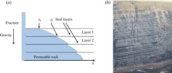
In the present work, we develop a complementary model for the buoyancy-driven flow through a horizontal multilayered formation in the limiting case in which the seal layers are continuous and hence in which there is no flux between the layers (figure 1 a). This situation has relevance as a model for deep sea turbidite fan deposits, in which multiple turbidite events can lead to the formation of a series of laterally extensive layers, each of order 1–10 m thick and interleaved with very-low-permeability clay or shale horizons which are 1–10 cm thick, as may be seen in the cliff outcrops at Loophead in County Clare, Ireland (figure 1 b). We focus on the role of buoyancy in controlling the flow within the different layers in order to model the dispersion associated with the layering. We first describe the flow that develops in each of the layers, and explore the effects of different numbers of layers in the formation. We then develop the analysis to describe the migration of a finite pulse of tracer which may be added as the flow evolves. We present a series of predictions of the model relating to the time evolution of the concentration of tracer downstream of the source, and develop a long-time model for the standard deviation of the tracer as a fraction of the position of the centre of mass of the tracer. Finally, we discuss the importance of the model predictions for pollutant dispersal. For simplicity we focus on the case of liquid migrating into an unsaturated rock, as would arise in the vadose zone above the main water table. However, we discuss the possible extension of the model to a fully saturated formation in the discussion.
2. A model of the flow
We consider an unsaturated formation consisting of
 $N$
horizontally extensive permeable layers, separated by very thin seal layers, each of thickness
 $H$
(figure 1). We assume that each of the layers has permeability
 $k$
and porosity
 ${\it\phi}$
and that the fluid entering the system has density
 ${\it\rho}$
and viscosity
 ${\it\mu}$
. We envisage that a vertical fracture intersects the formation and supplies fluid to each of the permeable layers from a constant pressure source with hydrostatic pressure
 ${\it\rho}gPH$
corresponding to an elevation
 $PH$
of the free surface of the source above the upper part of the formation, where
 $P$
is a dimensionless constant and
 $g$
is the acceleration of gravity.
(a) Schematic diagram of a generic layered formation with the intruding gravity current arising from a fracture that opens into each of the layers.
 $x_{s}$
and
 $x_{f}$
represent the contact point of the current with the top and the base of the layer. (b) Illustration of a layered turbidite rock, the Loophead cliff in County Clare, Ireland, showing a series of layers each of order 1–5 m thick and separated by thin layers of shale. The vertical scale of the cliff is approximately 40 m.

We assume that the resistance to flow in the fracture is small compared with that in the formation, and so the pressure at the top of the
 $n$
th layer is
 ${\it\rho}g[PH+(n-1)H]$
, where we count the layers from the top down. In general, the flow in the
 $n$
th layer will consist of a region near the fracture in which the layer is fully saturated with fluid, and beyond this there will be a gravity-driven nose which runs ahead as the current depth falls to zero (figure 1). In the
 $n\text{th}$
layer, in the region of current
 $x_{f}(t,n)>x>x_{s}(t,n)$
between the leading edge of the fully saturated region,
 $x_{s}(t,n)$
say, and the leading edge of the current,
 $x_{f}(t,n)$
say, we let the current have depth
 $h_{n}(x,t)$
. As the flow spreads out along the layers, we expect the leading part of the flow to become long and thin with scale
 $(x_{f}-x_{s})\gg H$
. Once this applies, we expect the velocity to become approximately horizontal and the vertical pressure gradient to become hydrostatic, leading to the local equation for the migration of the flow (cf. Huppert & Woods Reference Huppert and Woods1995),
 $$\begin{eqnarray}{\it\phi}\frac{\partial h_{n}}{\partial t}=\frac{k{\it\rho}g}{{\it\mu}}\frac{\partial }{\partial x}\left(h_{n}\frac{\partial h_{n}}{\partial x}\right),\end{eqnarray}$$
where the horizontal speed of the flow follows Darcy’s law. In these solutions, the flow continues to slump and spread with time; in § 3 we use the solutions to estimate the time beyond which the approximation
 $(x_{f}-x_{s})\gg H$
is valid.
In the region
 $0<x<x_{s}(t,n)$
, the layer is fully saturated and the Darcy flow speed is uniform, with value
 $u_{n}$
given by
 $$\begin{eqnarray}u_{n}=\frac{k(PH+(n-1)H){\it\rho}g}{x_{s}(t,n){\it\mu}}.\end{eqnarray}$$
This is related to the flux of fluid, per unit distance along the fracture, supplied to layer
 $n$
according to the relation
 $Q_{n}=u_{n}H$
. In the region
 $x_{s}<x<x_{f}$
, the current satisfies the boundary conditions
 $$\begin{eqnarray}\left(\frac{k{\it\rho}g}{{\it\mu}}\right)h_{n}\frac{\partial h_{n}}{\partial x}=Q_{n}\quad \text{at }x=x_{s}(t,n)\end{eqnarray}$$
and
 $h_{n}(x_{s},t)=1$
, while
 $h_{n}(x_{f},t)=0$
. On combining these relations we determine that there is a similarity solution with similarity variable
 ${\it\eta}$
defined by the relation
 $$\begin{eqnarray}x={\it\eta}\left(2SHt\right)^{1/2},\end{eqnarray}$$
where
 $S=(k{\it\rho}g)/({\it\mu}{\it\phi})$
. We define the function
 $f_{n}$
such that
 $h_{n}(x,t)=Hf_{n}({\it\eta})$
, so that
 $f_{n}$
is the shape function for the current. In the near-source region,
 ${\it\eta}\leqslant {\it\eta}_{s}$
, where
 $x_{s}={\it\eta}_{s}\left(2SHt\right)^{1/2}$
, we require
 $f_{n}({\it\eta}_{s})=1$
. However, in the gravity slumping nose region,
 ${\it\eta}_{s}<{\it\eta}<{\it\eta}_{f}$
, where
 ${\it\eta}_{f}=x_{f}/(2SHt)^{1/2}$
, we require
 $$\begin{eqnarray}-{\it\eta}\frac{\text{d}f_{n}}{\text{d}{\it\eta}}=\frac{\text{d}}{\text{d}{\it\eta}}\left(f_{n}\frac{\text{d}f_{n}}{\text{d}{\it\eta}}\right),\end{eqnarray}$$
with the boundary conditions
 $$\begin{eqnarray}\frac{\text{d}f_{n}}{\text{d}{\it\eta}}=-\!\left[\frac{P+n-1}{{\it\eta}_{s}}\right]\quad \text{at }{\it\eta}={\it\eta}_{s}\end{eqnarray}$$
and
 $f_{n}({\it\eta}_{f})=0$
.
This problem may be solved numerically to determine the relationship between
 ${\it\eta}_{s}$
,
 ${\it\eta}_{f}$
and the dimensionless hydrostatic pressure of the source,
 $P+(n-1)$
, acting on layer
 $n$
(cf. Li et al.
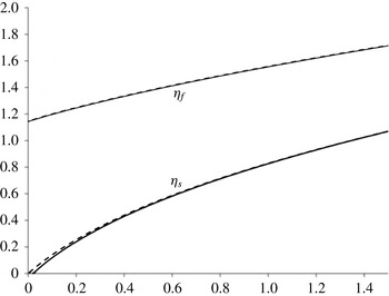
Reference Li, Lockington, Barry, Parlange and Perrochet2003). This is shown in figure 2, where the horizontal axis corresponds to
 $P+(n-1)$
and the dashed lines correspond to the full numerical solution for
 ${\it\eta}_{s}$
and
 ${\it\eta}_{f}$
.
For further analysis, it is convenient to note that (2.5) requires
 $\text{d}f_{n}/\text{d}{\it\eta}=-{\it\eta}$
at the front of the current where
 $f_{n}=0$
. Thus we can seek a power series expansion for
 $f_{n}({\it\eta})$
near
 ${\it\eta}={\it\eta}_{f}$
in the form
 $f_{n}({\it\eta})={\it\alpha}({\it\eta}_{f}-{\it\eta})+{\it\beta}({\it\eta}_{f}-{\it\eta})^{2}+{\it\gamma}({\it\eta}_{f}-{\it\eta})^{3}+\,\cdots$
, and this leads to the result
 $$\begin{eqnarray}f_{n}({\it\zeta})\approx {\it\eta}_{f}{\it\zeta}-\frac{1}{4}{\it\zeta}^{2}+\frac{2}{9{\it\eta}_{f}}{\it\zeta}^{3}+\cdots \,.\end{eqnarray}$$
On combining (2.7) with the boundary conditions we then find that this approximate solution predicts
 $$\begin{eqnarray}\left(P+n-1\right)\approx 2({\it\eta}_{f}^{2}-1)-{\it\eta}_{f}({\it\eta}_{f}^{2}-1)^{1/2}\end{eqnarray}$$
and
 $$\begin{eqnarray}{\it\eta}_{s}\approx 2({\it\eta}_{f}^{2}-1)^{1/2}-{\it\eta}_{f}.\end{eqnarray}$$
In figure 2 we also show the approximate solutions for
 ${\it\eta}_{s}$
and
 ${\it\eta}_{f}$
as solid lines. These are nearly indistinguishable from the full numerical solutions (dashed lines), suggesting that for modelling the properties of the flow, our analytic approximation provides a very accurate simplification. We also note from figure 2 that given that
 ${\it\eta}_{f}-{\it\eta}_{s}$
is of order
 $1$
, then it follows that
 $(x_{f}-x_{s})/H\sim (2St/H)^{1/2}$
. This has a value much larger than 1 for times
 $t\gg H/S$
. This is therefore the limit in which the present gravity-driven flow model provides an accurate description of the flow. In a typical permeable rock, with
 $S\sim 10^{-5}{-}10^{-7}~\text{m}~\text{s}^{-1}$
and
 $H\sim 1{-}10~\text{m}$
, this suggests that the present model applies for times in excess of weeks to months.
In a multilayer permeable rock, with a series of layers of thickness
 $H$
, the intruding gravity-driven flow increases in magnitude in the deeper layers. By moving in increments of
 $1$
on the horizontal axis of figure 2, from the initial value
 $P$
, we can infer the values
 ${\it\eta}_{s}(n,P)$
and
 ${\it\eta}_{f}(n,P)$
, for
 $n=2,3,\dots$
corresponding to successively deeper layers in the formation. The total flux,
 $F$
, in a formation with
 $N$
layers, of total thickness
 $NH$
, is given by the expression
 $$\begin{eqnarray}F=\left(\frac{SH}{(2SHt)^{1/2}}\right)\mathop{\sum }_{i=1}^{N}\frac{(P+(i-1))}{{\it\eta}_{s}(i,P)}.\end{eqnarray}$$
This may be compared with
 $F_{1}$
, the flux in a single layer of thickness
 $NH$
, driven by the same head
 ${\it\rho}gPH$
, which is given by
 $$\begin{eqnarray}F_{1}=\left(\frac{SNH}{(2SNHt)^{1/2}}\right)\frac{P}{{\it\eta}_{s}(1,P)}.\end{eqnarray}$$
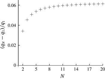
In figure 3 we illustrate that as the number of layers,
 $N$
, increases, while keeping
 $NH$
a constant, the total flux increases to a value approximately 6 % larger than the flux in a single layer, in the case
 $P=0$
. As
 $P$
increases to values
 $P>0$
this difference decreases towards zero. It is remarkable that this difference is so small; in the field it would be difficult to distinguish between these two systems based on measurements of the flux for a given head
 $P$
.
Variation of
 ${\it\eta}_{f}$
and
 ${\it\eta}_{s}$
as a function of
 $P+n-1$
, with the solid lines corresponding to the asymptotic solution and the dashed lines corresponding to the full numerical solution.

Variation of the flux in an
 $N$
-layered formation, in which each layer has the same depth
 $H$
, where
 $NH$
is a constant, relative to the flux in a one-layer formation of depth
 $NH$
, normalised by the flux in the one-layer formation. As
 $N$
increases and the layers become progressively thinner the flux increases to a maximum of 6 % in excess of the single-layer case.

3. Analogue Hele-Shaw experiments
We tested the predictions of the model using a vertical Hele-Shaw cell 10 cm high, 100 cm long and with a gap width of
 $d=2.5~\text{mm}$
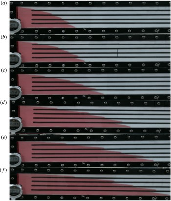
(as described by King & Woods Reference King and Woods2003). The top and the bottom of the cell were sealed and four narrow impermeable baffles were placed inside, thus dividing the cell into five layers. The whole vertical extent of one end of the cell was connected to a 5 l reservoir filled with red-dyed glycerol. A lock gate separated the cell from the reservoir as the reservoir tank was filled with glycerol to a level equal to or in excess of the height of the top of the cell. The cell was placed on a horizontal surface and at the start of the experiment, the lock gate between the end of the cell and the reservoir was removed so that glycerol could flow freely into the empty cell. The glycerol level in the reservoir was carefully maintained at a constant level by regularly topping it up, in order to provide a constant head for the flow.
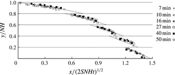
Figure 4 shows a succession of pictures taken from a typical experiment, for the case
 $P=0$
.
(a–f) Photographs of the gradual spreading of a gravity current in a five-layer Hele-Shaw cell, in which there is a source reservoir of constant depth. Photographs were taken 48, 591, 772, 1625, 2367 and 3643 s after the start of the experiment. For scale, the vertical height of the darker zone of fluid between the upper and lower boundaries of the cell, at the left-hand end of the cell, is 10 cm.

Comparison of the experimental data for the height of the current as a function of the distance from the source, in each of five layers, with the theoretical prediction. The distances have been scaled so that the vertical axis shows the quantity
 $y/NH$
and the horizontal axis shows the quantity
 $x/(2SNHt)^{1/2}$
. Here,
 $N=5$
and
 $H$
is the depth of each of the layers. The experimental data at each different time are shown by symbols which are defined in the legend on the graph.

For convenience, in figure 5, the horizontal position of the flow front in these experimental figures has been rescaled to the value
 $x/(2SNHt)^{1/2}$
, and the vertical position from the base of the cell has been rescaled to the value
 $y/NH$
, where
 $H$
is the thickness of one of the flow channels and
 $N=5$
. It is seen that the profiles at six different times collapse to the same line, and that these correspond to the theoretical prediction (§ 2) shown by the solid lines. In comparing the experiments with the model, we use the properties of glycerol, so that the density
 ${\it\rho}=1.26~\text{g}~\text{cm}^{-3}$
, the viscosity
 ${\it\mu}=1.2~\text{Pa}~\text{s}$
and the cell permeability
 $k=d^{2}/12=5.2~\text{mm}^{2}$
.
4. Migration of a pulse of dye in the flow
We now turn to the dispersion associated with the flow. In modelling the dispersion of a pulse of tracer or contaminant in a flow, there are a range of scales over which the dispersion can occur, and many models have been developed to describe dispersion in pressure-driven flows (Bear & Cheng Reference Bear and Cheng2010). Among other effects, models have explored the effects of anomalies in the dispersivity due to no-slip effects and dead-end pores for example (Saffman Reference Saffman1959; Young & Jones Reference Young and Jones1991), as well as the impact of large-scale heterogeneities in the formation, such as lenses of low or high permeability, which divert the flow (Eames & Bush Reference Eames and Bush1999; Dagan, Fiori & Jankovic Reference Dagan, Fiori and Jankovic2003). However, in a nearly uniform porous medium, the small-scale mechanical dispersion associated with the tortuous path round individual grains depends on the size of the grains
 ${\it\delta}$
and the flow speed
 $u$
(Phillips Reference Phillips1991; Bijelic, Muggeridge & Blunt Reference Bijelic, Muggeridge and Blunt2004; Delgado Reference Delgado2007), leading to a correlation for the longitudinal dispersion coefficient of the form
 $$\begin{eqnarray}D\sim (1.8\pm 0.4)({\it\delta}u)^{{\it\alpha}},\end{eqnarray}$$
where many experimental results suggest
 ${\it\alpha}\sim 1.0{-}1.2$
(Delgado Reference Delgado2007). In the case that the fluid advances along the permeable layer according to the self-similar flow model described above, the speed scales as
 $u\sim (SH/t)^{1/2}$
and so a localised region of tracer will spread dispersively by a longitudinal distance
 $L\sim {\it\delta}^{1/2}\left(SHt\right)^{1/4}$
, taking as a simplification the relation
 ${\it\alpha}\approx 1$
. In the following analysis we explore the mechanical dispersion of a cloud of tracer released into this layered medium. Once we have determined the rate of spreading of the cloud, we then show that at long times this dominates the longitudinal mechanical dispersion within each layer, as given in terms of the pore-scale longitudinal dispersion coefficient above.
In the present flow problem with a nearly horizontal gravity-driven flow (§ 2), then, in a single layer, the flow speed is independent of depth. Hence, in each layer we anticipate that any longitudinal dispersion will mirror the longitudinal dispersion associated with the formation (cf. (4.1)). However, in a multilayer system of depth
 $NH$
, with
 $N$
layers each of depth
 $H$
, as considered in § 3, the flow speed in the different layers varies with the depth of the layer (cf. figure 5). As a result, if some contaminant is released into the flow at a time
 $t_{o}$
, it will travel at different speeds in the different layers. In comparison to a single permeable layer of depth
 $NH$
, this will lead to longitudinal spreading of the contaminant. We now explore this macroscopic process, using the results from § 3.
We envisage that at time
 $t_{o}$
after the initial release of the flow from the pressurised source, a contaminant is released into the flow, and migrates downstream with the flow. In layer
 $i$
, the flow is characterised by the values
 ${\it\eta}_{f}(i,P)$
and
 ${\it\eta}_{s}(i,P)$
, and we can follow the trajectory of the dye,
 $x(i,t)$
, in layer
 $i$
by solving the relation
 $$\begin{eqnarray}\frac{\text{d}x}{\text{d}t}=\frac{u}{{\it\phi}},\end{eqnarray}$$
where the flow speed in the region where the aquifer is fully flooded is given by
 $$\begin{eqnarray}u=\frac{(P+i-1){\it\phi}SH}{{\it\eta}_{s}(2SHt)^{1/2}}\quad \text{for }x<{\it\eta}_{s}(2SHt)^{1/2}\end{eqnarray}$$
and in the gravity slumping zone it is given by
 $$\begin{eqnarray}u=-\frac{{\it\phi}SH}{(2SHt)^{1/2}}\frac{\text{d}f_{i}}{\text{d}{\it\eta}}\quad \text{for }{\it\eta}_{f}<x/(2SHt)^{1/2}<{\it\eta}_{s},\end{eqnarray}$$
where
 $f_{i}$
corresponds to layer
 $i$
. The analytical approximation for
 $f_{i}({\it\eta})$
(2.7) leads to the approximation
 $$\begin{eqnarray}\frac{\text{d}f_{i}}{\text{d}{\it\eta}}\approx -\frac{1}{2}{\it\eta}_{f}-\frac{1}{2}{\it\eta},\end{eqnarray}$$
so that (4.6) can be re-expressed in the form
 $$\begin{eqnarray}u=\frac{{\it\phi}SH}{2(2SHt)^{1/2}}\left({\it\eta}_{f}+\frac{x}{(2SHt)^{1/2}}\right)\quad \text{for }{\it\eta}_{f}<x/(2SHt)^{1/2}<{\it\eta}_{s},\end{eqnarray}$$
leading to the equation
 $$\begin{eqnarray}\frac{\text{d}x}{\text{d}t}=\frac{1}{2}\left(\frac{SH}{2t}\right)^{1/2}{\it\eta}_{f}+\frac{x}{4t}\end{eqnarray}$$
once the tracer has reached the gravity slump zone of the flow, with solution
 $$\begin{eqnarray}x(t)=\frac{{\it\eta}_{f}}{2}(2SHt)^{1/2}\left(1-\left(\frac{t_{1}}{t}\right)^{1/4}\right)+x_{1}\left(\frac{t}{t_{1}}\right)^{1/4},\end{eqnarray}$$
where
 $x_{1}$
is the time for the dye to reach the gravity slump zone after being released at
 $x=0$
at time
 $t_{o}$
, which follows from (4.3),
 $$\begin{eqnarray}x_{1}=\frac{(P+i-1){\it\phi}(2SHt_{1})^{1/2}}{{\it\eta}_{s}}\left(1-\left(\frac{t_{o}}{t_{1}}\right)^{1/2}\right).\end{eqnarray}$$
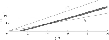
Characteristic diagram illustrating the migration of a pulse of dye with time, following release from the point
 $x=0$
in the lower layer of a two-layer formation. The
 $x$
axis shows the dimensionless quantity
 $\hat{t}^{1/2}=(St/H)^{1/2}$
while the
 $y$
axis shows the position downstream of the source scaled with the depth of the two layers,
 $\hat{x}=x/2H$
. In this calculation,
 $P=1$
and the dye pulse is released between times
 $\hat{t}=1$
and
 $\hat{t}=2$
.

These relations may be used to follow the trajectory of the dye in each layer, and this is shown in figure 6, where we illustrate the migration downstream of a parcel of dye in the lower layer of a two-layer formation as a function of
 $\hat{t}^{1/2}$
. The dye is released between the times
 $\hat{t}=St/H=1$
and
 $\hat{t}=St/H=2$
. As expected, the dye travels more rapidly than the leading edge of the fully saturated zone, labelled as the line
 $\hat{x}_{s}=x_{s}/2H$
, since the gravity slumping region grows in area with time, and so eventually the dye advances into the gravity slumping zone of the flow, whose leading edge is denoted by the line labelled
 $\hat{x}_{f}=x_{f}/2H$
in the figure.
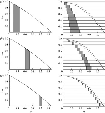
In a multilayer formation, the solutions illustrate the buoyancy-driven dispersion of a pulse of dye. For example, in figure 7 we show the case of a 10-layer formation in which a pulse of dye is released between the dimensionless times
 $\hat{t}=St/NH=1$
and
 $\hat{t}=2$
. We assume that each layer has thickness
 $H$
, and the migration of the dye pulse is compared with that in a single-layer formation of thickness
 $NH$
, where
 $N=10$
. Figure 7 illustrates the position of the dye in each layer at three different dimensionless times,
 $\hat{t}=St/NH$
. Since the flow is greater in the lower layers, these also have a larger pulse of dye. In the figure, the dimensionless vertical scale
 ${\hat{h}}=y/NH$
, where
 $N=10$
and
 $H$
is the thickness of each layer, while the horizontal position
 ${\it\eta}$
is the dimensionless position, which for convenience is defined by
 ${\it\eta}=x/(2SNHt)^{1/2}$
, which is the dimensionless scale for a current in a single layer of thickness
 $NH$
. Although initially the dye zones in successive layers overlap, as the flow travels downstream, and the gravity slump zone at the head of the flow spreads out, the regions of dye in each layer become separated in space. This is in sharp contrast to the case of the uniform single layer of depth
 $NH$
in which the dye pulse remains localised in space.
Comparison of the dispersal of a finite slug of tracer released during the dimensionless time interval
 $\hat{t}=St/NH=1$
to
 $\hat{t}=2$
in a single-layer formation of depth
 $NH$
and an
 $N$
-layer formation, in which each layer has depth
 $H$
, where
 $N=10$
. The position of the slug of dye is shown at three dimensionless times,
 $\hat{t}=St/NH$
, namely
 $\hat{t}=3$
(a), 12 (b) and 225 (c). The horizontal axis shows the dimensionless distance,
 ${\it\eta}=(2SNHt)^{1/2}$
, and the
 $y$
axis shows the vertical position scaled relative to
 $NH$
, as given by
 ${\hat{h}}=y/NH$
.

The longitudinal spreading of the dye pulse can be described in terms of the distribution relative to the centre of mass. The volume flux of dye supplied to each layer scales with the volume flux in each layer, and that is proportional to
 $(P+i-1)/{\it\eta}_{s}(i)$
for layer
 $i$
, while the approximate solution for the position of the dye (4.8) suggests that at long times, the position in layer
 $i$
scales as
 ${\it\eta}_{f}(i)$
. At long times, the centre of mass of the dye pulse is then given approximately by the relation ((2.6) and (2.7))
 $$\begin{eqnarray}\frac{\overline{x}}{(2SHt)^{1/2}}\sim \frac{\displaystyle \mathop{\sum }_{i=1}^{N}{\it\eta}_{f}(i)({\it\eta}_{f}(i)+{\it\eta}_{s}(i))}{\displaystyle \mathop{\sum }_{i=1}^{N}({\it\eta}_{f}(i)+{\it\eta}_{s}(i))},\end{eqnarray}$$
while the sum of the squares of the deviation from the centre of mass is given by
 $$\begin{eqnarray}\frac{({\rm\Delta}x)^{2}}{2SHt}=\mathop{\sum }_{i=1}^{N}\frac{(x_{i}-\overline{x})^{2}}{(2SHt)}\sim \frac{\displaystyle \mathop{\sum }_{i=1}^{N}{{\it\eta}_{f}(i)}^{2}({\it\eta}_{f}(i)+{\it\eta}_{s}(i))}{\displaystyle \mathop{\sum }_{i=1}^{N}({\it\eta}_{f}(i)+{\it\eta}_{s}(i))}-\frac{\overline{x}^{2}}{2SHt}.\end{eqnarray}$$
In the limit of a large number of layers,
 $N$
, and with an overpressure of the source large compared with the pressure drop across a single layer in the formation,
 $P\gg 1$
, it follows from (2.8) and (2.9) that
 $$\begin{eqnarray}{\it\eta}_{f(i)}\sim (P+i+1/2)^{1/2}\quad \text{and}\quad {\it\eta}_{s(i)}\sim {\it\eta}_{f(i)}-\frac{1}{{\it\eta}_{f(i)}},\end{eqnarray}$$
leading to the approximate relations, based on the summations in (4.10) and (4.11), that
 $$\begin{eqnarray}\frac{\overline{x}}{(2SNHt)^{1/2}}\sim \frac{3}{4N^{1/2}}\frac{(P+N+\frac{1}{2})^{2}-(P+\frac{1}{2})^{2}}{(P+N+\frac{1}{2})^{3/2}-(P+\frac{1}{2})^{3/2}}\end{eqnarray}$$
and
 $$\begin{eqnarray}\frac{({\rm\Delta}x)^{2}}{2SNHt}\sim \frac{3}{5N}\left(\frac{(P+N+\frac{1}{2})^{5/2}-(P+\frac{1}{2})^{5/2}}{(P+N+\frac{1}{2})^{3/2}-(P+\frac{1}{2})^{3/2}}\right)-\left(\frac{\overline{x}}{(2SNHt)^{1/2}}\right)^{2}.\end{eqnarray}$$
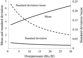
In the example case
 $P=N$
corresponding to a background overpressure equal to the hydrostatic pressure change across the depth of the formation, these relations lead to the prediction that with
 $N=20$
,
 $$\begin{eqnarray}\frac{{\rm\Delta}x}{\overline{x}}\sim 0.095,\end{eqnarray}$$
and in general the values of these predictions are illustrated in figure 8 for a 20-layer aquifer, as a function of the dimensionless overpressure of the source,
 $P$
. Equations (4.13) and (4.14) identify that for large
 $N$
both
 $\overline{x}$
and
 ${\rm\Delta}x$
scale with
 $(2SNHt)^{1/2}$
, and this implies that the buoyancy-driven dispersion continues at the same rate as the dye pulse advances through the aquifer, so that at long times, the longitudinal distribution of the dye has a length scale that is a constant fraction of the distance travelled by the centre of mass of the dye. In contrast to these results, if there was just one layer in the formation, the dye would travel with the speed of the centre of mass, and, other than the mechanical pore-scale dispersion, cf. (4.1), the dye pulse would remain relatively localised.
Our analysis has identified that the mechanical dispersion associated with the difference in speeds of the flow in the different layers leads to a cloud of tracer spreading over a distance of order
 $L\sim (SHt)^{1/2}$
as a function of time. At long times, this is much faster than the in-layer longitudinal dispersion
 $L\sim ({\it\delta}^{1/2}(SHt)^{1/4})$
, and it begins to dominate the in-layer dispersion after a time of order
 $t\sim {\it\delta}^{2}/SH$
. In a typical formation, with grains of order 0.1 mm in size, and a flow speed of
 $10^{-7}~\text{m}~\text{s}^{-1}$
, this implies that the interlayer dispersion begins to dominate after a time of the order of seconds in a layer of thickness 1 m.
Comparison of the position of the centre of mass (solid; left-hand axis) and of the variance of the slug of tracer about the centre of mass (solid; left-hand axis) and of the ratio of the standard deviation to the mean (dashed line; right hand axis).

5. Discussion
We have examined the gravity-driven flow produced by a constant pressure source which supplies fluid to a multilayer geological formation. We have demonstrated that there is a variation in the lateral speed of the flow between successive layers, with the flux and flow speed increasing downwards as the pressure increases. We have shown that the flux supplied to such a system is only a few per cent larger than the flux supplied to a single layer of comparable thickness, depending on the source overpressure. However, if there is a finite release of contaminant or tracer into the flow, then this will be dispersed by the flow in the multilayer formation. We have shown that in the long-time limit, this dispersion leads to a spreading of the pulse of dye so that the longitudinal distribution of contaminant has a length scale that is directly proportional to the centre of mass of the contaminant, and has a magnitude of order 0.1 of the position of the centre of mass, suggesting that for such flows, the effective dispersion coefficient increases with the scale of the flow.
This result may be important in helping to interpret measurements of the location of a tracer that becomes dispersed within a buoyancy-driven flow. For example, if water is injected into the shallow subsurface to clean up a light non-aqueous phase liquid or other spill, it may be of value to use a tracer in the flow to determine the different flow paths and the flow rate. The modelling presented herein suggests that if there is an observation well or producing well, and this is used to measure the passage of the tracer, then the effects of buoyancy-driven dispersion may lead to substantial longitudinal dispersion in a plume of tracer. Eventually the plumes of tracer in each of the layers may become separated in space (see figure 7), so that an observation well sufficiently far downstream would only record intermittent pulses of tracer. In contrast to the case of multiple layers, if there was a single layer, then the buoyancy-driven flow would be uniform and so would not lead to such dispersal of a pulse of tracer.
Although the flow is an idealisation, if we consider a shallow permeable formation with 10 layers of thickness 5 m, and a permeability of
 $0.1\times 10^{(-12)}~\text{m}^{2}$
, then the buoyancy-driven flow speed would be of order
 $S\sim 10^{-5}$
. After a period of
 $10^{7}~\text{s}$
(about four months), for example corresponding to rain water ingress and longitudinal spreading during a wet season, the flow would have travelled a distance of order 100 m, and a finite pulse of tracer in this flow would have spread out through buoyancy-driven dispersion by an amount of order 10–20 m. With grain sizes of 0.1 mm the effective longitudinal dispersion coefficient (4.1) would be of order
 $10^{-8}{-}10^{-9}~\text{m}^{2}~\text{s}^{-1}$
, suggesting that, over this time, the pore-scale dispersion would lead to spreading of the dye pulse by an amount of order 0.1–1.0 m, which is small compared with the buoyancy-driven dispersal described herein.
There are numerous other geometries that one may envisage which are subject to buoyancy-driven dispersion, including a vertical flow through a fracture, and we are presently exploring such flows. It would also be of interest to extend the present analysis to consider the case of dispersion by a gravity-driven flow in a layered formation already saturated with fluid. In that case, the principles will be analogous to the present study, although the detailed flow field will be different. Finally, we mention that in a number of situations in which contaminants spread through the subsurface, the rheology of the fluids may be non-Newtonian, leading to a different flow rate as a function of the driving pressure (Ciriello et al. Reference Ciriello, Di Federico, Archetti and Longo2013; Di Federico et al. Reference Di Federico, Longo, Chiapponi, Archetti and Ciriello2014). Again, the dispersion resulting from the interlayer differences in flow rate associated with the buoyancy, as described in the present work, will persist, although for each specific rheology the detailed flow structure will be different. We are presently exploring some extensions of the present work for that context.
Acknowledgements
We are grateful for funding from the NDA and the EU Forge programme and we thank S. Norris for continuing support of the work.