1. Introduction
Both robots and inertial measurement units (IMUs) must be calibrated to perform accurately in a host of applications. Traditionally, they are calibrated independently using highly accurate, often cumbersome, and typically expensive dedicated systems. The motivation for our work is to eliminate all external measurement systems and calibrate the robot and IMU simultaneously simply by attaching the IMU to the robot’s end-effector and moving the robot around continuously throughout its workspace.
Robot calibration itself is the process of estimating updates to the robot’s kinematic model parameters, based on a set of observations of the end-effector pose. Calibration’s ability to make substantial improvements to robot accuracy is supported by a rich and mature body of literature [Reference Roth, Mooring and Ravani1–Reference He, Zhao, Yang and Yang5].
Widely used in mobile and aerial robotics applications, IMUs provide real-time measurements of the kinematic state of a system useful for online estimation and feedback control. Their micro-electro-mechanical systems (MEMS) typically include some combination of triaxial accelerometers, gyroscopes, and magnetometers. These systems are compact and manufactured as a single integrated circuit, making them inexpensive and integrable into the majority of robotic systems. However, the MEMS sensors in IMUs present a set of intrinsic parameters that must be calibrated. Nonzero sensor biases, nonunit scale factors, and sensor axis misalignments should all be identified prior to IMU use [Reference Fong, Ong and Nee6–Reference Tedaldi, Pretto and Menegatti9]. Furthermore, the spatial relationships (i.e. the rotation and translation) between the IMU and the robot’s coordinate system must be determined prior to use in real-time robot estimation or monitoring applications.
Data collection for IMU calibration is often less straightforward than for robot calibration. This is because – neglecting the potential triaxial magnetometer – IMU calibration typically consists of two subproblems: accelerometer and gyroscope calibration. In a laboratory setting, the standard methodology for calibration of IMUs requires mounting the IMU on a leveled turntable [Reference Poddar, Kumar and Kumar10]. The turntable is then commanded to a precise angular rate, and the IMU sensors are sampled. Comparing the gyroscope and accelerometer outputs to known values based on the speed of the leveled turntable and Earth’s gravity enables calibration.
Calibration methods have been proposed that do not require a turntable, for example, based on using the Earth’s angular velocity or gravity [Reference Fong, Ong and Nee6, Reference Tedaldi, Pretto and Menegatti9]. These methods, while promising, are less accurate than turntable methods and are often unable to calibrate the gyroscope parameters due to numerical issues. Thus, “expensive mechanical platforms are often inevitable” [Reference Rohac, Sipos and Simanek11] for IMU calibration. IMU parameters also drift over time and must be periodically re-calibrated [Reference Poddar, Kumar and Kumar10], making availability and use of dedicated turntable solutions undesirable. This is especially undesirable in robotics applications since this would require removal of the IMU, mounting on a turntable for calibration, and reinstallation into the robot system.
By combining the IMU and robot calibration together, we eliminate the need for such specialized and time-consuming calibration steps for each system individually. Furthermore, our method completely eliminates additional calibration steps for the extrinsic IMU parameters (e.g. determining the pose of the IMU relative to the robot). This is all accomplished in one fast calibration step with no external equipment.
In this paper, we propose a new method to estimate the many parameters involved when mounting an IMU onto a serial robot’s end-effector without any external equipment (i.e. “self-calibration”). The robot’s joint position sensors and data output from the IMU are sampled while the robot moves continuously. The resulting time series is used to infer the following sets of parameters: (i) robot kinematic parameters, (ii) IMU intrinsic parameters (i.e. sensor gains, biases, and misalignments), and (iii) extrinsic parameters (i.e. sensor rotations, translation, temporal offset, and gravity). Enabled by recent advancements in continuous-time batch estimation [Reference Furgale, Tong, Barfoot and Sibley12], our method computes maximum a posteriori (MAP) estimates of the system parameters and the trajectory simultaneously given the sampled data. Under Gaussian assumptions, we show that this leads to a nonlinear least-squares problem and analyze the structure of the associated Jacobian. Finally, as the planned robot trajectory is arbitrary, we devise a sequential method for numerically planning the trajectory that improves estimation convergence. Our sequential approach makes solutions to a computationally intractable trajectory planning problem feasible. We validate our methods in simulation and with experimental data collected with an AUBO i5 industrial robot (AUBO Robotics, USA) comparing our calibration to standard methods for both robot and IMU calibration.
Our unified calibration approach is useful for three main scenarios. First, our approach enables (i) a fast and inexpensive alternative to traditional robot calibration. While the method is evidently useful for estimating robot angle parameters (i.e. a Level I and partial Level II robot calibration [Reference Roth, Mooring and Ravani1]), our numerical results provide evidence suggesting that full Level II robot calibration (with length parameters) is possible given a sufficiently fast robot trajectory. Robot calibration equipment (e.g. optical/laser tracking systems) is often expensive, and data collection is often cited as the most time-consuming part of calibration [Reference Elatta, Gen, Zhi, Daoyuan and Fei13]. The IMU used in our experiments cost less than 30 USD, and automatic data collection took only 5 min. Furthermore, the method does not require any line of sight such is the case with optical tracking systems. Second, our approach enables (ii) a fast, cheap, and automated alternative to traditional IMU calibration. Specifically, our method circumvents the need for expensive external calibration equipment (e.g. rate tables) provided that a robot is available.
Finally, our method enables (iii) an essential calibration step for online robot estimation and monitoring applications using IMUs. For example, IMUs have been explored as a primary means of measuring robot joint angles [Reference Cheng and Oelmann14–Reference Roan, Deshpande, Wang and Pitzer17]. More recently, data from IMUs have been fused with joint position sensor data to increase robot accuracy online [Reference Olofsson, Antonsson, Kortier, Bernhardsson, Robertsson and Johansson18, Reference Munoz-Barron, Rivera-Guillen, Osornio-Rios and Romero-Troncoso19]; this approach could be especially useful to improve the accuracy of compliant [Reference Burgner-Kahrs, Rucker and Choset20] or cable-driven [Reference Le, Do and Phee21] medical robots. Additionally, IMUs have been used for robot collision monitoring [Reference Birjandi, Kühn and Haddadin22] and could be applied to general fault detection. In order to use an IMU in these applications, many extrinsic parameters (e.g. rotation and translation of the IMU relative to the end-effector) must first be determined. Furthermore, our method eschews removal of the IMU from the robot to achieve an accurate IMU calibration; this is especially useful since frequent recalibration of sensor parameters is often unavoidable [Reference Poddar, Kumar and Kumar10].
2. Related work on robot/IMU calibration
While IMUs have seen extensive application in mobile robotics, their use has been more limited in fixed-base robot manipulators. Here, we outline related works concerning calibration with IMU-equipped stationary robots in three general categories.
2.1. Robot calibration via IMU
Robot calibration is typically carried out measuring end-effector pose; however, some groups have instead attempted to use IMU data for robot calibration. Perhaps the earliest example is ref. [Reference Canepa, Hollerbach and Boelen23] where the method showed promise; however, the achieved end-effector error was on the order of 15 mm. More recently, in ref. [Reference D’Amore, Ciarleglio and Akin24] the achieved positioning errors were still large in comparison to typical requirements. While these studies laid the foundation for IMU-based robot calibration, our method achieves better accuracy while additionally estimating many other useful parameters.
Others have adopted a sensor fusion approach to IMU-based robot calibration. In ref. [Reference Du and Zhang25], the authors use a Kalman filter fusion algorithm to estimate the end-effector orientation. The orientations alone were then used to calibrate the robot. While the accuracy of the robot was improved in this case, it is not possible to estimate the robot length parameters from orientation information alone. Thus, in refs. [Reference Du26, Reference Du, Liang, Li, Liu and Li27], the authors fuse data from both an IMU and a position sensor to estimate the full pose of the end-effector. An unscented Kalman filter was then used to estimate the robot kinematic errors online from the pose information. Even though the authors achieved good accuracy results, the position sensor used adds another operating constraint (line of sight) to the robot, while an IMU alone poses minimal constraint.
Importantly, in all of these works, IMU measurements were taken under static conditions. In our method, we sample the data while the robot moves continuously. These data collected under dynamic conditions are potentially more informative. During motion, we can measure the acceleration and angular velocity of the end-effector. If, on the other hand, the robot is stationary, these quantities are all zero.
Furthermore, in order to use an IMU for robot calibration, its sensor parameters must first be calibrated. In each of the aforementioned works, the IMU sensors were either calibrated beforehand or nominal values were used instead, potentially sacrificing accuracy. Our method proposes to jointly estimate the robot and IMU parameters in one fast and accurate calibration step.
2.2. IMU calibration via robot
While IMU calibration is typically conducted using turntables, some researchers have instead opted to use robot data. In ref. [Reference Renk, Rizzo, Collins, Lee and Bernstein28], the authors present a method using a robot to calibrate an end-effector-mounted accelerometer and magnetometer. Similarly, in ref. [Reference Botero-Valencia, Marquez-Viloria, Castano-Londono and Morantes-Guzmán29], the authors present an open source, low cost robot for calibration of IMUs. In ref. [Reference Beravs, Podobnik and Munih30], the authors focus on calibration of the triaxial accelerometer portion of the IMU using a serial robot.
These methods were able to calibrate at least some of the IMU sensors using a robot arm with good results. However as the robot was not in motion during data collection, many of the gyroscope parameters could not be estimated. In our proposed dynamic method, we are able to calibrate all of the sensor parameters of interest. Furthermore, our method also simultaneously calibrates the robot; this makes our method potentially more accurate.
2.3. Sensor extrinsic calibration
While most applications of IMUs in robotics are limited to visual-inertial navigation and mobile robots [Reference Qin, Li and Shen31–Reference Forster, Carlone, Dellaert and Scaramuzza37], some researchers have instead attempted to use IMU data with stationary robots. For example, some researchers have used inertial sensors for joint angle measurement instead of traditional angle transducers (e.g. encoders) [Reference Cheng and Oelmann14]. In ref. [Reference Ghassemi, Tafazoli, Lawrence and Hashtrudi-Zaad15], the authors measure the joint angles of a robot using 2 axis accelerometers with a static accelerometer calibration scheme to estimate voltage biases. Similarly, in ref. [Reference Cantelli, Muscato, Nunnari and Spina16], the authors propose a method for estimating joint angles of an industrial robot using multiple IMUs. In order to use the sensors for estimation, several of the gyroscope parameters were first calibrated by moving the robot dynamically; the accelerometer parameters were then calibrated while the robot was stationary by comparing the sensor outputs to gravity. In ref. [Reference Roan, Deshpande, Wang and Pitzer17], the authors use IMUs for joint angle estimation with good results. A necessary step was the calibration of the sensor spatial offset which was only briefly discussed.
More recently, researchers have fused joint position sensor data and IMU data together to increase robot accuracy [Reference Olofsson, Antonsson, Kortier, Bernhardsson, Robertsson and Johansson18, Reference Munoz-Barron, Rivera-Guillen, Osornio-Rios and Romero-Troncoso19]. Toward this, in ref. [Reference Olofsson, Antonsson, Kortier, Bernhardsson, Robertsson and Johansson18], the researchers present a calibration method to estimate the spatial offset of the IMU relative to the end-effector. Their sensor fusion methods did improve robot accuracy; however, accuracy could be further improved using our method which also estimates the relevant IMU and robot parameters.
3. Robot and inertial sensor models
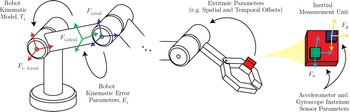
Our method involves a fixed-base serial robot moving along a trajectory while sampling data from an end effector-mounted IMU. In this section, models describing how the system’s parameters affect measurement outputs are developed in order to facilitate self-calibration of the system. An overview of the system parameters involved is illustrated in Fig. 1.
Diagram of a serial robot with end-effector-mounted inertial measurement unit (IMU) illustrating the various parameters and reference frames involved. Given known robot motion, IMU outputs can be predicted; however, these predictions will in general be erroneous due to unknown errors in robot kinematic parameters, IMU intrinsic parameters, and extrinsic parameters relating the two. Our calibration method determines all of these parameters simultaneously given robot and IMU data sampled during continuous motion.

3.1. Serial robot model
We adopt the generalized kinematic error method in ref. [Reference Meggiolaro and Dubowsky38] to model the kinematics of serial robots and to parameterize their kinematic errors. We use this method because compared to the Denavit–Hartenberg (DH) error parameterization, it has been shown to be minimal (i.e. no error parameter redundancy), continuous (small changes in error parameters
 $\implies$
small changes in robot geometry), and complete (enough parameters to describe any deviation from nominal) [Reference He, Zhao, Yang and Yang5] for any serial robot geometry without any additional modifications [Reference Hayati and Mirmirani39].
Under this method, the robot link transform between frame
 $F_{i-1,\text{real}}$
and frame
 $F_{i,\text{ideal}}$
(see Fig. 1) is first computed using the standard DH convention
 \begin{equation} T_i = \begin{bmatrix} \cos \theta _i & \quad -\cos \alpha _i \sin \theta _i & \quad \sin \alpha _i \sin \theta _i & \quad a_i \cos \theta _i \\[4pt] \sin \theta _i & \quad \cos \theta _i \cos \alpha _i & \quad -\sin \alpha _i \cos \theta _i & \quad a_i \sin \theta _i \\[4pt] 0 & \quad \sin \alpha _i & \quad \cos \alpha _i & \quad d_i \\[4pt] 0 & \quad 0 & \quad 0 & \quad 1 \end{bmatrix} \end{equation}
where
 $\theta _i$
,
 $d_i$
,
 $a_i$
,
 $\alpha _i$
are the joint angle offset, the joint offset, link length, and link twist of link
 $i$
, respectively. These DH parameters are the same both before and after calibration.
Rather than using the DH convention to parameterize the kinematic errors, each link transform is modified by six generalized error parameters
 $\epsilon _{i_1}, \epsilon _{i_2}, \epsilon _{i_3}, \epsilon _{i_4}, \epsilon _{i_5}, \epsilon _{i_6}$
where the first three parameters describe translation along the
 $X, Y, \text{and } Z$
axes, respectively, and the last three correspond to a
 $YZX$
Euler rotation sequence. Thus, the error transform between frame
 $F_{i,\text{ideal}}$
and frame
 $F_{i,\text{real}}$
(see Fig. 1) is given by
 \begin{equation} E_i = \begin{bmatrix} c_4 c_5 & \quad s_6 s_4 - c_6 c_4 s_5 & \quad c_6 s_4 + c_4 s_6 s_5 & \quad \epsilon _{i_1} \\[4pt] s_5 & \quad c_6 c_5 & \quad -c_5 s_6 & \quad \epsilon _{i_2} \\[4pt] -c_5 s_4 & \quad c_4 s_6 + c_6 s_4 s_5 & \quad c_6 c_4 - s_6 s_4 s_5 & \quad \epsilon _{i_3} \\[4pt] 0 & \quad 0 & \quad 0 & \quad 1 \end{bmatrix} \end{equation}
where, for example,
 $c_4$
stands for
 $\cos \epsilon _{i_4}$
, and
 $s_6$
stands for
 $\sin \epsilon _{i_6}$
. Kinematics computation of the rotation and translation (
 $R \in \text{SO}(3)$
and
 $\boldsymbol{{p}} \in \mathbb{R}^3$
, respectively) of the IMU board attached to the robot end-effector is carried out by multiplying all of the transforms together in order
 \begin{equation} \begin{bmatrix} R & \quad \boldsymbol{{p}} \\[4pt] \textbf{0}^\intercal & \quad 1 \end{bmatrix} = E_0 T_1 E_1 \dots T_n E_n \end{equation}
where we note that the transform
 $E_0$
has been added to describe the pose of the robot base frame relative to a world frame. Additionally, in our setup,
 $E_n$
describes the pose of the IMU frame relative to the end-effector.
Given the functions
 $\boldsymbol{{q}}, \dot{\boldsymbol{{q}}}, \ddot{\boldsymbol{{q}}} \,:\, \mathbb{R} \mapsto \mathbb{R}^n$
, we can predict the angular velocity
 $\boldsymbol{\omega }_n$
and linear acceleration
 $\boldsymbol{{a}}_n$
of the IMU frame relative to the robot base using the familiar Newton recurrence relationship
 \begin{align} \begin{split} \boldsymbol{\omega }_{i+1} &= \boldsymbol{\omega }_i + \boldsymbol{{n}}_{z_i} \dot{q_i}(t) \\ \boldsymbol{\alpha }_{i+1} &= \boldsymbol{\alpha }_i + \boldsymbol{{n}}_{z_i} \ddot{q_i}(t) + \boldsymbol{\omega }_i \times (\boldsymbol{{n}}_{z_i} \dot{q_i}(t)) \\ \boldsymbol{{v}}_{i+1} &= \boldsymbol{{v}}_i + \boldsymbol{\omega }_{i+1} \times \boldsymbol{\rho }_{i+1} \\ \boldsymbol{{a}}_{i+1} &= \boldsymbol{{a}}_i + \boldsymbol{\alpha }_{i+1} \times \boldsymbol{\rho }_{i+1} + \boldsymbol{\omega }_{i+1} \times (\boldsymbol{\omega }_{i+1} \times \boldsymbol{\rho }_{i+1}) \end{split} \end{align}
where
 $\boldsymbol{\rho }_i$
is the distance vector between frame
 $i$
and frame
 $i-1$
and
 $\boldsymbol{{n}}_{z_i}$
is the direction of the
 $Z$
axis of frame
 $i$
as computed in the DH model (3). Note that this calculation also gives the angular acceleration
 $\boldsymbol{\alpha }_i$
and linear velocity
 $\boldsymbol{{v}}_i$
for each of the robot links. Transforming these quantities from the robot base frame into the IMU frame and adding the force of gravity to the computed acceleration, we get the predicted inertial quantities
 \begin{align} \begin{split} \boldsymbol{\omega }(t) &= R^\intercal \boldsymbol{\omega }_n \\ \boldsymbol{{s}}(t) &= R^\intercal (\boldsymbol{{a}}_n - \boldsymbol{{g}}) \end{split} \end{align}
where
 $\boldsymbol{{s}}$
and
 $\boldsymbol{\omega }$
are the specific force and angular velocity, respectively, acting on the sensor and
 $R$
is the rotation of the IMU frame relative to the robot base computed in (3). Note that because the magnitude of the gravity vector
 $\boldsymbol{{g}}$
is known to be 9.81 m/s
 $^2$
, we parameterize
 $\boldsymbol{{g}}$
with only two values
 $\boldsymbol{{g}}_{xy} = [g_x g_y]^\intercal$
.
3.2. Inertial sensor model
We use the inertial sensor model in ref. [Reference Zhang, Wu, Wu, Wu and Hu8] to describe how angular velocity
 $\boldsymbol{\omega }$
and specific force
 $\boldsymbol{{s}}$
map to raw voltage values. This model accounts for nonunit sensor gains, nonorthogonal sensitivity axes, nonzero sensor voltage biases, and gross sensor rotations relative to the IMU frame. Note that the position of the IMU frame relative to the robot end-effector has already been accounted for by
 $E_n$
in (3).
The model that we use which relates the inertial quantities
 $\boldsymbol{\omega }(t)$
and
 $\boldsymbol{{s}}(t)$
to sensor voltages is
 \begin{align} \begin{split} \tilde{\boldsymbol{\omega }}(t) &= K_\omega \Gamma _\omega R_\omega \boldsymbol{\omega }(t) + \boldsymbol{{b}}_\omega \\ \tilde{\boldsymbol{{s}}}(t) &= K_a \Gamma _a R_a \boldsymbol{{s}}(t) + \boldsymbol{{b}}_a \end{split} \end{align}
where
 \begin{alignat*}{3} \Gamma _a & = \begin{bmatrix} 1 & \quad 0 & \quad 0 \\[4pt] \gamma _{a_{yz}} & \quad 1 & \quad 0 \\[4pt] -\gamma _{a_{zy}} & \quad \gamma _{a_{zx}} & \quad 1 \end{bmatrix}&, \quad\quad \Gamma _\omega & = \begin{bmatrix} 1 & \quad 0 & \quad 0 \\[4pt] \gamma _{\omega _{yz}} & \quad 1 & \quad 0 \\[4pt] -\gamma _{\omega _{zy}} & \quad \gamma _{\omega _{zx}} & \quad 1 \end{bmatrix}&, \quad\\[4pt] K_a & = \begin{bmatrix} k_{a_x} & \quad 0 & \quad 0 \\[4pt] 0 & \quad k_{a_y} & \quad 0 \\[4pt] 0 & \quad 0 & \quad k_{a_z} \end{bmatrix}&, \quad\quad K_\omega & = \begin{bmatrix} k_{\omega _x} & \quad 0 & \quad 0 \\[4pt] 0 & \quad k_{\omega _y} & \quad 0 \\[4pt] 0 & \quad 0 & \quad k_{\omega _z} \end{bmatrix}. \end{alignat*}
Here,
 $\tilde{\boldsymbol{\omega }}$
and
 $\tilde{\boldsymbol{{s}}}$
are the output voltages caused by the IMU frame’s angular velocity
 $\boldsymbol{\omega }(t)$
and specific force
 $\boldsymbol{{s}}(t)$
, respectively. Note that noise will be added to these ideal outputs
 $\tilde{\boldsymbol{\omega }}$
and
 $\tilde{\boldsymbol{{s}}}$
in our full measurement model (10).
The rotation matrix
 $R_\omega$
accounts for the gross rotational misalignment of the triaxial gyroscope on the IMU frame and is parameterized by a
 $ZYX$
Euler angle sequence with parameters
 $(r_{\omega _z}, r_{\omega _y}, r_{\omega _x})$
. The matrix
 $R_a$
is similar, but is for the accelerometer and has parameters
 $(r_{a_z}, r_{a_y}, r_{a_x})$
. The lower triangular matrices
 $\Gamma _\omega$
and
 $\Gamma _a$
account for small gyroscope and accelerometer sensor axis misalignments to first order. The diagonal matrices
 $K_\omega$
and
 $K_a$
are gains which map the physical quantities to voltage values.
Finally, the vectors
 $\boldsymbol{{b}}_\omega$
and
 $\boldsymbol{{b}}_a$
are the triaxial sensor biases (nonzero voltage offsets) for the gyroscope and accelerometer, respectively. In this paper, we assume that these parameters are constant. To assess the validity of this assumption with our IMU, we performed a test where we collected IMU data for 25 min, 5 times longer than our experiments. To check for drift in the values
 $\boldsymbol{{b}}_\omega$
and
 $\boldsymbol{{b}}_a$
, we filtered the IMU data using a smoothing spline and then computed the error between the spline and the mean. The maximum drift observed was 0.017 m/s
 $^2$
for the accelerometer and 0.025
 $^\circ$
/s for the gyroscope. Both of these values are well within the range of the sensor noise computed in Section 8. This analysis verifies the assumption of constant sensor biases in our specific setup. However, when sensor biases drift significantly, continuous-time functions for
 $\boldsymbol{{b}}_\omega$
and
 $\boldsymbol{{b}}_a$
can be neatly folded into the estimation problem [Reference Furgale, Tong, Barfoot and Sibley12, Reference Furgale, Rehder and Siegwart40].
3.3. Parameter redundancy
There are currently
 $6 (n + 1)$
generalized error parameters in the robot kinematic model (3). However, this is currently not a minimal set of parameters. In other words, there are directions in
 $\epsilon$
-space which have no effect on the computed IMU location
 $T$
in (3). Following the method in ref. [Reference Meggiolaro and Dubowsky38], several of these redundancies must be eliminated prior to calibration. If
 $\boldsymbol{\epsilon }_0 = \{ \epsilon _{0_1} \dots \epsilon _{0_6} \quad \epsilon _{1_1} \dots \epsilon _{1_6} \quad \dots \quad \epsilon _{n_1} \dots \epsilon _{n_6} \} \in \mathbb{R}^{6(n + 1)}$
is the set of all generalized error parameters, the subset
 $\boldsymbol{\epsilon } \subset \boldsymbol{\epsilon }_0$
is the minimal set of parameters.
In ref. [Reference Meggiolaro and Dubowsky38], the authors provide a comprehensive and systematic approach for determining the subset
 $\boldsymbol{\epsilon }$
depending on whether the end-effector pose measurements include both position and orientation. Therefore, based on ref. [Reference Meggiolaro and Dubowsky38], the length of the robot kinematic error vector is at most
 $6(n + 1) - 2 N_r - 4 N_p$
, where
 $N_r$
is the number of revolute joints and
 $N_p$
is the number of prismatic joints.
Furthermore, it is important to note that in our IMU–robot arrangement, the IMU can only provide motion information relative to itself or relative to the robot. This means that the transform from the robot base to the world system
 $E_0$
is not identifiable from the IMU measurements. Because of this, we do not include the parameters
 $\epsilon _{0_1}, \epsilon _{0_2}, \ldots, \epsilon _{0_6}$
in
 $\boldsymbol{\epsilon }$
. Finally, we note that the rotation parameters
 $\epsilon _{n_4}, \epsilon _{n_5}, \text{and}\ \epsilon _{n_6}$
that describe the orientation of the IMU frame are redundant with the each of the sensor orientations
 $R_\omega$
and
 $R_a$
. Therefore, we eliminate these parameters as well. After elimination of these redundant parameters, the length of
 $\boldsymbol{\epsilon }$
is
 $6n - 2N_r - 4N_p - 3$
.
Together with the robot parameters
 $\boldsymbol{\epsilon }$
, 12 gyroscope parameters, 12 accelerometer parameters, 2 gravity direction parameters, and the time offset
 $\tau$
, there are
 $6n - 2N_r - 4N_p + 24$
system parameters that we pack into the vector
 $\boldsymbol{{x}}$
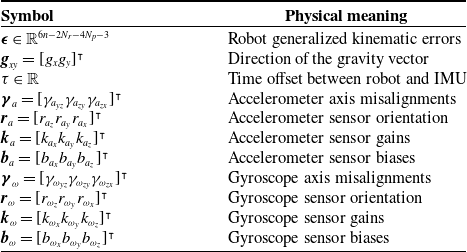
. Table I details the components of the vector
 $\boldsymbol{{x}}$
.
System parameter vector
 $\boldsymbol{{x}}$
for the serial robot–IMU system.

4. Bayesian parameter estimation
4.1. Problem statement
In our method, instead of taking measurements at static configurations, the IMU is sampled while the robot moves continuously through the trajectory
 $\boldsymbol{{q}} \,:\, \mathbb{R} \mapsto \mathbb{R}^n$
. During robot motion, IMU outputs
 $\boldsymbol{{z}}_i$
are sampled at times
 $t_i$
and the robot joint transducer outputs
 $\boldsymbol{{q}}_j$
are sampled at times
 $t_j$
where
 $i = 1 \dots N_z$
,
 $j = 1 \dots N_q$
, and
 $N_z$
,
 $N_q$
are the number of IMU measurements and the number of joint vector measurements, respectively. Note that we do not assume synchronous measurements of
 $\boldsymbol{{z}}_i$
and
 $\boldsymbol{{q}}_j$
. The set of all IMU outputs
 $\boldsymbol{{z}}_{1:N_z}$
and the set of all joint vector measurements
 $\boldsymbol{{q}}_{1:N_q}$
are then used optimally to infer the system parameters
 $\boldsymbol{{x}}$
and the robot trajectory
 $\boldsymbol{{q}}(t)$
simultaneously. Here, we roughly follow ref. [Reference Furgale, Tong, Barfoot and Sibley12] to derive an estimator.
4.2. Posterior parameter distribution
All of the information that the measurements
 $\boldsymbol{{z}}_{1:N_z}$
and
 $\boldsymbol{{q}}_{1:N_q}$
can reveal about the system parameters
 $\boldsymbol{{x}}$
and the robot trajectory
 $\boldsymbol{{q}}(t)$
is encoded in the posterior probability distribution
 $p\!\left(\boldsymbol{{x}}, \boldsymbol{{q}}(t) \mid \boldsymbol{{q}}_{1:N_q}, \boldsymbol{{z}}_{1:N_z}\right)$
. Bayes’ theorem asserts that this distribution takes the form
 \begin{equation} { p\!\left(\boldsymbol{{x}}, \boldsymbol{{q}}(t) \mid \boldsymbol{{q}}_{1:N_q}, \boldsymbol{{z}}_{1:N_z}\right) = \frac{ p\!\left(\boldsymbol{{q}}_{1:N_q}, \boldsymbol{{z}}_{1:N_z} \mid \boldsymbol{{x}}, \boldsymbol{{q}}(t)\right) p(\boldsymbol{{x}}, \boldsymbol{{q}}(t)) }{ p\!\left(\boldsymbol{{q}}_{1:N_q}, \boldsymbol{{z}}_{1:N_z}\right) }. } \end{equation}
If we assume that the data
 $\boldsymbol{{q}}_{1:N_q}$
,
 $\boldsymbol{{z}}_{1:N_z}$
and the system parameters
 $\boldsymbol{{x}}$
are all statistically independent from the inputs
 $\boldsymbol{{q}}(t)$
, then the expression on the right becomes
 \begin{equation} \frac{ p\!\left(\boldsymbol{{q}}_{1:N_q}, \boldsymbol{{z}}_{1:N_z} \mid \boldsymbol{{x}}\right) p(\boldsymbol{{x}}) p(\boldsymbol{{q}}(t)) }{ p\!\left(\boldsymbol{{q}}_{1:N_q}, \boldsymbol{{z}}_{1:N_z}\right) }. \end{equation}
Additionally assuming that the input measurements
 $\boldsymbol{{q}}_{1:N_q}$
are independent of the IMU data
 $\boldsymbol{{z}}_{1:N_z}$
leads to
 \begin{equation} { p\!\left(\boldsymbol{{x}}, \boldsymbol{{q}}(t) \mid \boldsymbol{{q}}_{1:N_q}, \boldsymbol{{z}}_{1:N_z}\right) = \frac{ p(\boldsymbol{{q}}_{1:N_q} \mid \boldsymbol{{x}}) p(\boldsymbol{{z}}_{1:N_z} \mid \boldsymbol{{x}}) p(\boldsymbol{{x}}) p(\boldsymbol{{q}}(t)) }{ p\!\left(\boldsymbol{{q}}_{1:N_q}, \boldsymbol{{z}}_{1:N_z}\right) }. } \end{equation}
4.3. Conditional and prior distribution assumptions
In order to make the estimation problem feasible, we must make statistical assumptions about the distributions of the measured data. As is often done, we assume a zero-mean, Gaussian measurement model for both the joint vector samples and the IMU outputs:
 \begin{equation} \begin{alignedat}{2} \boldsymbol{{q}}_j &= \boldsymbol{{q}}(t_j) + \boldsymbol{{n}}_{q,j}, \quad &\boldsymbol{{n}}_{q,j} \sim \mathcal{N}\left(\textbf{0}, \Sigma _{q_j}\right) \\ \boldsymbol{{z}}_i &= \boldsymbol{{h}}(t_i + \tau, \boldsymbol{{x}}) + \boldsymbol{{n}}_{z,i}, \quad &\boldsymbol{{n}}_{z,i} \sim \mathcal{N}\left(\textbf{0}, \Sigma _{z_i}\right) \end{alignedat} \end{equation}
where
 $\boldsymbol{{n}}_{q,j}$
and
 $\boldsymbol{{n}}_{z,i}$
are zero-mean Gaussian random vectors with covariance
 $\Sigma _{q_j}$
and
 $\Sigma _{z_i}$
. Here, the function
 $\boldsymbol{{h}} \,:\, \left(\mathbb{R} \times \mathbb{R}^{6n - 2r - 4p + 24}\right) \mapsto \mathbb{R}^6$
stacks the vectors
 $\tilde{\boldsymbol{{s}}}(t)$
and
 $\tilde{\boldsymbol{\omega }}(t)$
and is dependent on the function
 $\boldsymbol{{q}}(t)$
. Equation (10) implies that the conditional distributions of the data are
 \begin{align} \begin{split} p(\boldsymbol{{q}}_j \mid \boldsymbol{{x}}) &\sim \mathcal{N}\!\left(\boldsymbol{{q}}(t_j), \Sigma _{q_j}\right) \\ p(\boldsymbol{{z}}_i \mid \boldsymbol{{x}}) &\sim \mathcal{N}\!\left(\boldsymbol{{h}}(t_i + \tau, \boldsymbol{{x}}), \Sigma _{z_i}\right). \end{split} \end{align}
We also assume that the prior distribution of the system parameters is independent and Gaussian:
 \begin{equation} p(\boldsymbol{{x}}) \sim \mathcal{N}(\hat{\boldsymbol{{x}}}, \Sigma _{\hat{x}}). \end{equation}
where
 $\hat{\boldsymbol{{x}}}$
are the nominal parameters and
 $\Sigma _{\hat{x}}$
is the assumed covariance of the nominal parameters (e.g. from known measurement or manufacturing error).
The final assumption is that the prior distribution of the joint value function
 $p(\boldsymbol{{q}}(t))$
over the joint space is constant and uniform for all time. In other words, we assume that there is no prior information about the robot trajectory. Given these assumptions, the posterior distribution (9) is proportional to a product of Gaussians where the constant of proportionality does not depend on either
 $\boldsymbol{{x}}$
or
 $\boldsymbol{{q}}(t)$
. In particular, the proportionality can be expressed as
 \begin{equation} p\!\left(\boldsymbol{{x}}, \boldsymbol{{q}}(t) \mid \boldsymbol{{q}}_{1:N_q}, \boldsymbol{{z}}_{1:N_z}\right) \propto p(\boldsymbol{{x}}) \prod _{j=1}^{N_q} p(\boldsymbol{{q}}_j \mid \boldsymbol{{x}}) \prod _{i=1}^{N_z} p(\boldsymbol{{z}}_i \mid \boldsymbol{{x}}). \end{equation}
4.4. MAP formulation
The MAP estimate seeks to minimize the negative logarithm of the posterior distribution, as this is equivalent to maximization of the distribution:
 \begin{equation} (\boldsymbol{{x}}^*, \boldsymbol{{q}}^*(t)) = \underset{\boldsymbol{{x}}, \boldsymbol{{q}}(t)}{\arg \min } \left\{{-}\log\! \left(p\!\left(\boldsymbol{{x}}, \boldsymbol{{q}}(t) \mid \boldsymbol{{q}}_{1:N_q}, \boldsymbol{{z}}_{1:N_z}\right)\right)\right\}. \end{equation}
Given the Gaussian assumptions, (13) shows that the objective function in (14) can be expanded into the following quadratic form in the unknowns
 $\boldsymbol{{x}}$
and
 $\boldsymbol{{q}}(t)$
:
 \begin{equation} -\log\!\left(p\!\left(\boldsymbol{{x}}, \boldsymbol{{q}}(t) \mid \boldsymbol{{q}}_{1:N_q}, \boldsymbol{{z}}_{1:N_z}\right)\right) = c + J_q + J_z + J_x \end{equation}
where c is some constant that does not depend on the system parameters
 $\boldsymbol{{x}}$
or the joint vector function
 $\boldsymbol{{q}}(t)$
and
 \begin{align} \begin{split} J_q &= \frac{1}{2} \sum _{j = 1}^{N_q} \boldsymbol{{e}}_{q_j}^{\intercal } \Sigma _{q_j}^{-1} \boldsymbol{{e}}_{q_j} \\[3pt] \boldsymbol{{e}}_{q_j} &= \boldsymbol{{q}}_j - \boldsymbol{{q}}(t_j) \\[3pt] J_z &= \frac{1}{2} \sum _{i = 1}^{N} \boldsymbol{{e}}_{z_i}^{\intercal } \Sigma _{z_i}^{-1} \boldsymbol{{e}}_{z_i} \\[3pt] \boldsymbol{{e}}_{z_i} &= \boldsymbol{{z}}_i - \boldsymbol{{h}}(t_i + \tau, \boldsymbol{{x}}) \\[3pt] J_x &= \boldsymbol{{e}}_x^\intercal \Sigma _{\hat{x}}^{-1} \boldsymbol{{e}}_x \\[3pt] \boldsymbol{{e}}_x &= \boldsymbol{{x}} - \hat{\boldsymbol{{x}}} \end{split} \end{align}
Defining
 $J(\boldsymbol{{x}}, \boldsymbol{{q}}(t)) = J_q + J_z + J_x$
, we note that because the constant
 $c$
does not depend on the optimization variables, the solution to
 \begin{equation} (\boldsymbol{{x}}^*, \boldsymbol{{q}}^*(t)) = \underset{\boldsymbol{{x}}, \boldsymbol{{q}}(t)}{\arg \min }\{J(\boldsymbol{{x}}, \boldsymbol{{q}}(t))\} \end{equation}
is the same as the MAP estimate (14). Therefore, solving the optimization problem (17) leads to the MAP estimate of the system parameters
 $\boldsymbol{{x}}$
and the trajectory
 $\boldsymbol{{q}}(t)$
.
5. Trajectory representation
Currently, along with the parameter vector
 $\boldsymbol{{x}}$
, one of the unknowns in the optimization problem (17) is a function
 $\boldsymbol{{q}}(t)$
. If we are to have any hope of computing a solution, we must first agree on a representation of
 $\boldsymbol{{q}}(t)$
that a computer can evaluate. Usually, continuous functions are approximated as a sum of basis functions, but the particular basis functions used are a design choice. We follow refs. [Reference Furgale, Tong, Barfoot and Sibley12, Reference Furgale, Rehder and Siegwart40] and choose to use B-splines as a basis to represent the unknown function
 $\boldsymbol{{q}}(t)$
.
There are two main advantages to this choice of basis for continuous-time batch estimation [Reference Furgale, Tong, Barfoot and Sibley12]. One is that B-splines are locally supported. In other words, the contribution of any single basis function is local in time. This is useful for solving problems like (17) because the changes in the state trajectory caused by a change in a B-spline coefficient are zero almost everywhere. This makes for a sparse Jacobian and thus efficient nonlinear least-squares solutions. Second, there are simple and efficient algorithms for evaluating B-spline functions, derivatives, and integrals [Reference Schumaker41] – quantities which are necessary for evaluation of the objective function (17).
We choose to represent the robot trajectory
 $\boldsymbol{{q}}(t)$
as linear combinations of B-splines following the general methodology of ref. [Reference Schumaker41]. Given spline degree
 $d$
, smoothness
 $d - 1$
, and time points
 $a = x_0 \lt x_1 \lt \cdots \lt x_k \lt x_{k+1} = b$
in an interval
 $\Omega = [a, b]$
, the extended partition
 $\Delta _e = \{y_i\}_{i = 1}^{n + d + 1}$
is defined to be
 \begin{equation} \begin{gathered} a = y_1 = \ldots = y_{d + 1}, \\ y_{n + 1} = \ldots = y_{n + d + 1} = b, \\ y_{d + 2} \leq \dots \leq y_n = x_1, \dots x_k, \end{gathered} \end{equation}
where the dimension of the spline space can be shown to be
 $m = k + d + 1$
. Given this extended partition
 $\Delta _e$
, in one dimension, we represent functions as linear combinations of the normalized B-splines:
 \begin{equation} f(t) = \sum _{i = 1}^m c_i N_i^{d + 1}(t) \end{equation}
where
 $f$
is any function in the spline space, the
 $N_i^{d + 1}(t)$
are the normalized B-splines of order
 $d + 1$
, and the
 $c_i$
are the multiplying coefficients which determine the shape of the function
 $f(t)$
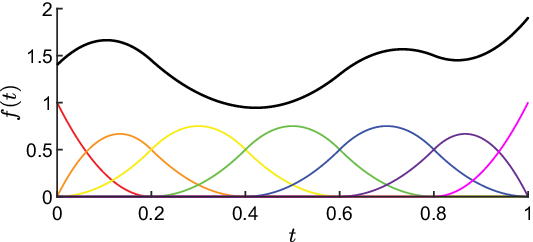
. An example function is shown in Fig. 2.
B-Spline function representation. The normalized B-splines
 $\{N_i^{3}(t)\}_{i = 1}^7$
are shown in color. The function
 $f(t)$
which is a linear combination (
 $\boldsymbol{{c}} = [1.4 \; 1.9 \; 1.0 \; 0.9 \; 1.7 \; 1.3 \; 1.9]^\intercal$
) of the B-splines is shown in black. The B-splines make for efficient function evaluation and differentiation, and their local support makes for efficient solving of continuous-time trajectory estimation problems.

Extending this representation to
 $n$
dimensions, we can write curves such as the robot trajectory in (17) using the following matrix equation:
 \begin{equation} \boldsymbol{{q}}(t) = C \boldsymbol{{N}}^{d + 1}(t) = \begin{bmatrix} c_{11} & \quad c_{12} & \quad \cdots & \quad c_{1m} \\[4pt] c_{21} & \quad c_{22} & \quad & \quad \vdots \\[4pt] \vdots & \quad & \quad \ddots & \quad \vdots \\[4pt] c_{n1} & \quad \cdots & \quad \cdots & \quad c_{nm} \end{bmatrix} \begin{bmatrix} N_1^{d + 1}(t) \\[4pt] N_2^{d + 1}(t) \\[4pt] \vdots \\[4pt] N_m^{d + 1}(t) \\[4pt] \end{bmatrix}. \end{equation}
As the basis functions are known, if the matrix
 $C$
is known, then one way to calculate
 $\boldsymbol{{q}}(t)$
is by evaluating all of the B-splines that have value at the time point and then computing the linear combinations using (20).
However, a more efficient way to evaluate (20) which we adopt is to use the recurrence relationship outlined in ref. [Reference Schumaker41]. Additionally, we use a similar relationship (also outlined in ref. [Reference Schumaker41]) to compute the B-spline coefficients corresponding to the derivatives of (20),
 $\dot{\boldsymbol{{q}}}(t)$
and
 $\ddot{\boldsymbol{{q}}}(t)$
, from the matrix
 $C$
.
Finally, as mentioned earlier, one important advantage of the B-spline representation is its local support. Specifically, considering the interval
 $\Omega _i = [y_i, y_{i + d + 1}]$
,
 \begin{equation} \begin{split} &N_i^{d + 1}(t) \gt 0 \quad \text{for } y_i \lt t \lt y_{i + d + 1} \\ &N_i^{d + 1}(t) = 0 \quad \text{otherwise}. \end{split} \end{equation}
This is illustrated in Fig. 2 where each of the basis functions only take on nonzero values within a smaller subset of the total interval
 $[0, 1]$
. We exploit this fact in Section 7 where we iteratively plan trajectories to maximize parameter identifiability.
6. Least squares formulation
Our ultimate goal is to solve (17), determining estimates for the parameters
 $\boldsymbol{{x}}$
as well as the unknown actual trajectory
 $\boldsymbol{{q}}(t)$
. However, in light of the chosen trajectory representation (20), the new unknowns that we would like to estimate are
 $\boldsymbol{{x}}$
and
 $C$
. Writing the coefficient matrix
 $C$
as a vector
 $\boldsymbol{{c}} = [c_{11} \dots c_{n1} \quad \dots \quad c_{1m} \dots c_{nm}]^\intercal$
, and defining the full vector of unknowns
 $\boldsymbol{\theta } = [\boldsymbol{{x}}^\intercal \quad \boldsymbol{{c}}^\intercal ]^\intercal$
, the cost function in (17) can be rewritten in matrix form as
 \begin{equation} J(\boldsymbol{\theta }) = \frac{1}{2} \boldsymbol{{e}}^\intercal \Sigma _e^{-1} \boldsymbol{{e}} \end{equation}
where
 \begin{align*} \boldsymbol{{e}} & = \begin{bmatrix} \boldsymbol{{e}}_{q_1}^\intercal \cdots \boldsymbol{{e}}_{q_N}^\intercal & \quad \boldsymbol{{e}}_{z_1}^\intercal \cdots \boldsymbol{{e}}_{z_N}^\intercal & \quad \boldsymbol{{e}}_{x} \end{bmatrix} ^{\intercal } \\[4pt] \Sigma _e & = \text{blkdiag} \begin{bmatrix} \Sigma _{q_1} \cdots \Sigma _{q_{N_j}} & \quad \Sigma _{z_1} \cdots \Sigma _{z_{N_i}} & \quad \Sigma _x \end{bmatrix}. \end{align*}
The residual vector of (22) can be written as
 \begin{equation} \boldsymbol{\delta } = L \boldsymbol{{e}} \end{equation}
where
 $L$
is the Cholesky factor of
 $\Sigma _e^{-1}$
 $\left(\Sigma _e^{-1} = L^\intercal L\right)$
. Note that the Cholesky decomposition always exists in the case of symmetric, positive definite matrices like
 $\Sigma _e^{-1}$
.
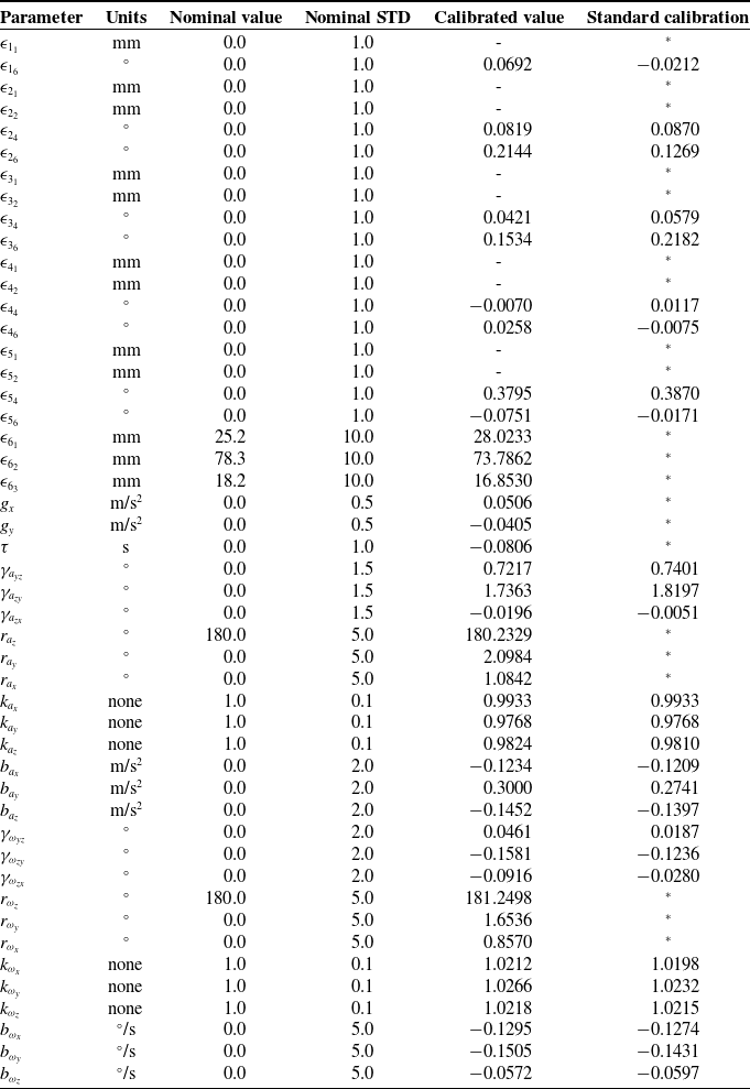
Nominal and calibrated model parameters
 $\boldsymbol{{x}}$
and their standard deviations in our experiments.

If a unique solution exists, this problem can be solved with any nonlinear least-squares solver such as the Levenberg–Marquardt (LM) algorithm. In order to prevent convergence to an incorrect local minimum, it is recommended to supply a good nominal guess to the algorithm. See Section 8.1 and Table II for an example showing how to determine nominal parameters and their prior uncertainties. Furthermore, if the solution is nearby to the nominal solution, the confidence in our estimate
 $\boldsymbol{\theta }^*$
is encoded in the posterior covariance matrix
 \begin{equation} \Sigma _\theta = \left( \left[\frac{\partial \boldsymbol{{e}}}{\partial \boldsymbol{\theta }}\right]^\intercal \Sigma _e^{-1} \frac{\partial \boldsymbol{{e}}}{\partial \boldsymbol{\theta }} \right)^{-1} \end{equation}
where
 $\frac{\partial \boldsymbol{{e}}}{\partial \boldsymbol{\theta }}$
is the identification Jacobian matrix associated with
 $\boldsymbol{\theta }$
. Note that least-squares solvers like LM generally benefit from providing a derivative to (23). In this case, assuming that
 $L$
is constant, differentiation of (23) results in
 \begin{equation} \frac{\partial \boldsymbol{\delta }}{\partial \boldsymbol{\theta }} = L \frac{\partial \boldsymbol{{e}}}{\partial \boldsymbol{\theta }}. \end{equation}
6.1. The structure of the Jacobian
In our experiments, solution of (22) was not feasible with standard, dense matrices. Here, we analyze the sparsity structure of
 $\dfrac{\partial \boldsymbol{{e}}}{\partial \boldsymbol{\theta }}$
determining which elements of the Jacobian are nonzero. Knowledge of this structure enables the use of sparse finite difference methods to compute
 $\dfrac{\partial \boldsymbol{{e}}}{\partial \boldsymbol{\theta }}$
making solution of (22) feasible.
First, we note that of the parameters
 $\boldsymbol{\theta } = [\boldsymbol{{x}}^\intercal \quad \boldsymbol{{c}}^\intercal ]^\intercal$
, the system parameters
 $\boldsymbol{{x}}$
only influence the output measurement errors
 $\boldsymbol{{e}}_z$
and cannot influence the input measurement errors
 $\boldsymbol{{e}}_q$
. Inspection of (16) verifies this;
 $\boldsymbol{{e}}_q$
is only a function of
 $\boldsymbol{{c}}$
, so
 $\dfrac{\partial \boldsymbol{{e}}_q}{\partial \boldsymbol{{x}}} = 0$
. In contrast, each component of the spline coefficients
 $\boldsymbol{{c}}$
can affect both
 $\boldsymbol{{e}}_q$
and
 $\boldsymbol{{e}}_z$
. However, the local support of B-splines (21) makes many of the elements of
 $\dfrac{\partial \boldsymbol{{e}}_q}{\partial \boldsymbol{{c}}}$
and
 $\dfrac{\partial \boldsymbol{{e}}_z}{\partial \boldsymbol{{c}}}$
zero. For measurements
 $\boldsymbol{{q}}_i$
taken at time
 $t_i \notin [y_j, y_{j + d + 1}]$
, the derivative of (21) is zero. Employing the chain rule on
 $\boldsymbol{{e}}_{q_i}$
in (16) shows that
 $\dfrac{\partial \boldsymbol{{e}}_{q_i}}{\partial \boldsymbol{{c}}_j} = 0$
. Similarly, the effect of
 $\boldsymbol{{c}}_j$
is local on
 $\boldsymbol{{e}}_z$
. A similar argument shows that for measurements
 $\boldsymbol{{z}}_i$
taken at time
 $(t_i + \tau ) \notin [y_j, y_{j + d + 1}]$
,
 $\dfrac{\partial \boldsymbol{{e}}_z}{\partial \boldsymbol{{c}}} = 0$
. Finally, a spline coefficient can only affect
 $\boldsymbol{{e}}_{q_i}$
if it is on the same row in the matrix (20), so
 $\dfrac{\partial \boldsymbol{{e}}_{q_i}}{\partial \boldsymbol{{c}}_j}$
can only have one nonzero element.
Next we note that the parameters in
 $\boldsymbol{\epsilon }$
which correspond to translational displacements cannot affect the orientation of the end-effector. Therefore, the model-predicted rate of orientation
 $\boldsymbol{\omega }$
also cannot be affected by such length parameters, so that
 $\dfrac{\partial \boldsymbol{{e}}_\omega }{\partial \boldsymbol{\epsilon }_i} = 0$
when
 $i \in \{1, 2, 3\}$
. As the gravity direction also does not affect measured orientations,
 $\dfrac{\partial \boldsymbol{{e}}_\omega }{\partial \boldsymbol{{g}}_{xy}} = 0$
.
Because of the way the sensor misalignments
 $\boldsymbol{\gamma }_a$
and
 $\boldsymbol{\gamma }_\omega$
are incorporated into the matrices
 $\Gamma _a$
and
 $\Gamma _\omega$
(6), the corresponding matrices
 $\dfrac{\partial \boldsymbol{{e}}_\omega }{\partial \boldsymbol{\gamma }_\omega }$
and
 $\dfrac{\partial \boldsymbol{{e}}_\alpha }{\partial \boldsymbol{\gamma }_\alpha }$
have sparsity structures
 \begin{equation*} \begin {bmatrix} 0 & \quad 0 & \quad 0 \\[4pt] * & \quad 0 & \quad 0 \\[4pt] 0 & \quad * & \quad * \end {bmatrix} \end{equation*}
where a
 $*$
indicates any nonzero element. Similarly, it can be shown that the
 $YZX$
Euler sequences
 $\boldsymbol{{r}}_a$
and
 $\boldsymbol{{r}}_\omega$
lead to the sparsity structure
 \begin{equation*} \begin {bmatrix} * & \quad * & \quad 0 \\[4pt] * & \quad 0 & \quad * \\[4pt] 0 & \quad * & \quad * \end {bmatrix} \end{equation*}
for the matrices
 $\dfrac{\partial \boldsymbol{{e}}_\omega }{\partial \boldsymbol{{r}}_\omega }$
and
 $\dfrac{\partial \boldsymbol{{e}}_\alpha }{\partial \boldsymbol{{r}}_\alpha }$
. As the gain matrices
 $K_a$
and
 $K_\omega$
are diagonal, and the sensor biases are just offsets,
 $\dfrac{\partial \boldsymbol{{e}}_\omega }{\partial \boldsymbol{{k}}_\omega }$
,
 $\dfrac{\partial \boldsymbol{{e}}_\alpha }{\partial \boldsymbol{{k}}_\alpha }$
,
 $\dfrac{\partial \boldsymbol{{e}}_\omega }{\partial \boldsymbol{{b}}_\omega }$
, and
 $\dfrac{\partial \boldsymbol{{e}}_\alpha }{\partial \boldsymbol{{b}}_\alpha }$
are all diagonal,
 $3 \times 3$
matrices. Finally, we note that the accelerometer parameters cannot affect the gyroscope outputs, and similarly, the gyroscope parameters cannot affect the accelerometer outputs; therefore, the following matrices are zero:
 $\dfrac{\partial \boldsymbol{{e}}_\omega }{\partial \boldsymbol{\gamma }_a}$
,
 $\dfrac{\partial \boldsymbol{{e}}_\omega }{\partial \boldsymbol{{r}}_a}$
,
 $\dfrac{\partial \boldsymbol{{e}}_\omega }{\partial \boldsymbol{{k}}_a}$
,
 $\dfrac{\partial \boldsymbol{{e}}_\omega }{\partial \boldsymbol{{b}}_a}$
,
 $\dfrac{\partial \boldsymbol{{e}}_\alpha }{\partial \boldsymbol{\gamma }_\omega }$
,
 $\dfrac{\partial \boldsymbol{{e}}_\alpha }{\partial \boldsymbol{{r}}_\omega }$
,
 $\dfrac{\partial \boldsymbol{{e}}_\alpha }{\partial \boldsymbol{{k}}_\omega }$
, and
 $\dfrac{\partial \boldsymbol{{e}}_\alpha }{\partial \boldsymbol{{b}}_\omega }$
.
For
 $\boldsymbol{{e}}_x$
,
 $\dfrac{\partial \boldsymbol{{e}}_x}{\partial \boldsymbol{{x}}}$
is an identity matrix of size
 $6n - 2r - 4p + 24$
and
 $\dfrac{\partial \boldsymbol{{e}}_x}{\partial \boldsymbol{{c}}}$
is a zero matrix with size
 $(6n - 2r - 4p + 24) \times nm$
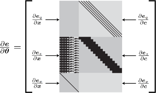
. A diagram showing an example sparsity structure of the full Jacobian
 $\dfrac{\partial \boldsymbol{{e}}}{\partial \boldsymbol{{x}}}$
can be seen in Fig. 3.
Sparsity pattern of the Jacobian matrix
 $\dfrac{\partial \boldsymbol{{e}}}{\partial \boldsymbol{\theta }}$
which can be exploited for efficient least-squares solutions. The labeled, gray submatrices combine to form the full block matrix
 $\dfrac{\partial \boldsymbol{{e}}}{\partial \boldsymbol{\theta }}$
. Black pixels indicate elements that are not necessarily zero, and gray pixels indicate entries that are always zero. In this example, we use only
 $N_i = N_j = 15$
data samples for visualization purposes, but in our experiments, we had over 30,000 samples leading to a Jacobian with greater than 99% sparsity.

This diagram was generated using the system in our experiments with 15 measurements of both
 $\boldsymbol{{q}}$
and
 $\boldsymbol{{z}}$
for visualization purposes. Note that with only 15 measurements,
 $\dfrac{\partial \boldsymbol{{e}}}{\partial \boldsymbol{\theta }}$
in Fig. 3 is only about 85% sparse, but it was greater than 99% sparse in our experiments where many thousands of measurements were taken.
7. Numerical trajectory planning
Even though part of our problem is to estimate the actual robot trajectory
 $\boldsymbol{{q}}$
, up to this point, the commanded robot trajectory
 $\tilde{\boldsymbol{{q}}}\, :\, \mathbb{R} \mapsto \mathbb{R}^n$
is still arbitrary. While we could command the joint values to follow any trajectory, we can reduce estimation error substantially by commanding a trajectory
 $\tilde{\boldsymbol{{q}}}$
that is in some sense optimal. Optimal trajectory planning has been used for identification of robot dynamic parameters for many years [Reference Swevers, Ganseman, Tukel, De Schutter and Van Brussel42, Reference Bonnet, Fraisse, Crosnier, Gautier, González and Venture43], but here we propose and test a new method that specifically deals with long trajectories, such as the 5 min timescale in our self-calibration problem.
7.1. Efficient approximation of the posterior covariance
Our ultimate goal is to estimate the parameter vector
 $\boldsymbol{{x}}$
, so our definition for optimality should ultimately serve to reduce the posterior estimation error
 $\Sigma _x$
. In order to develop an efficient approximation for
 $\Sigma _x$
, we momentarily assume that the actual robot trajectory
 $\boldsymbol{{q}}$
is close to the planned trajectory
 $\tilde{\boldsymbol{{q}}}$
(i.e.
 $\tilde{\boldsymbol{{q}}} = \boldsymbol{{q}}$
). This assumption is reasonable because robot controllers are generally accurate at following planned trajectories; furthermore, our numerical results show that, even with this assumption, our parameter estimates are about 10 times more precise than if random trajectories are used. Note that we verify the validity of this temporary approximation in our numerical experiments (Section 8). Given a trajectory plan
 $\tilde{\boldsymbol{{q}}}$
, the posterior covariance of
 $\boldsymbol{{x}}$
now takes the form
 \begin{equation} \Sigma _x = \left(\Sigma _{\hat{x}}^{-1} + \left[\frac{\partial \boldsymbol{{e}}_z}{\partial \boldsymbol{{x}}}\right]^\intercal \Sigma _z^{-1} \frac{\partial \boldsymbol{{e}}_z}{\partial \boldsymbol{{x}}} \right)^{-1}, \end{equation}
where
 $\Sigma _z = \text{blkdiag} [\Sigma _{z_1} \cdots \Sigma _{z_N}]$
and
 $\boldsymbol{{e}}_z = \left[\boldsymbol{{e}}_{z_1}^\intercal \cdots \boldsymbol{{e}}_{z_N}^\intercal \right]^\intercal$
.
Approximation of
 $\Sigma _x$
using (26) is significantly more efficient than computing
 $\Sigma _\theta$
with (24) and then extracting
 $\Sigma _x$
. In the former case, we only need to compute a Jacobian
 $\dfrac{\partial \boldsymbol{{e}}_z}{\partial \boldsymbol{{x}}}$
of size
 $6N_i \times 48$
(assuming a 6 axis rotary system). In the latter case, we would have to compute the matrix
 $\dfrac{\partial \boldsymbol{{e}}}{\partial \boldsymbol{\theta }}$
of size
 $(6N_j + 6N_i + 48) \times (48 + 6m)$
. Because
 $N_j$
and
 $m$
are generally quite large (e.g. 36,000 and 303 in our experiments), the matrix
 $\dfrac{\partial \boldsymbol{{e}}}{\partial \boldsymbol{\theta }}$
is much larger in both dimensions than
 $\dfrac{\partial \boldsymbol{{e}}_z}{\partial \boldsymbol{{x}}}$
. Therefore, as long as the approximation (26) is reasonably accurate, a significant efficiency advantage can be obtained by using (26) over (24) for the many thousands of computations of
 $\Sigma _x$
during trajectory planning.
7.2. Trajectory planning problem statement
To reduce posterior uncertainty, we want to make
 $\Sigma _x$
as small as possible in some sense by varying the B-spline coefficients
 $\boldsymbol{{c}}$
(and thus
 $\boldsymbol{{q}}(t)$
). It is well-known that the maximum singular value of
 $\Sigma _x$
provides an upper bound on the posterior variance of any parameter in
 $\boldsymbol{{x}}$
. Therefore, similar to ref. [Reference Swevers, Ganseman, Tukel, De Schutter and Van Brussel42], to reduce parameter uncertainty, we minimize the maximum singular value of
 $\Sigma _x$
. In particular, we solve the following optimization problem:
 \begin{equation} \boldsymbol{{c}}^* = \underset{\boldsymbol{{c}}}{\arg \min }\{\max \text{svd} (\Sigma _x)\} \\ \end{equation}
subject to
 \begin{equation} \boldsymbol{{q}}_{\text{min}} \leq \begin{bmatrix} \boldsymbol{{q}}(t) \\[4pt] \dot{\boldsymbol{{q}}}(t) \\[4pt] \ddot{\boldsymbol{{q}}}(t) \end{bmatrix} \leq \boldsymbol{{q}}_{\text{max}} \quad \text{for all } t, \end{equation}
where the vectors
 $\boldsymbol{{q}}_{\text{min}}$
and
 $\boldsymbol{{q}}_{\text{max}}$
constrain the trajectory by setting upper and lower bounds on the joint values, velocities, and accelerations.
Solving (27) using the approximation (26) should ensure a good trajectory for data collection. However, in order to achieve good results, the data collection process must proceed over several minutes. In our experiments, this long trajectory corresponds to a
 $\boldsymbol{{c}}$
with length 1818. With an objective function (27) taking several seconds to compute, solution of this large-scale, inequality-constrained, nonlinear trajectory optimization problem was not feasible on our research PC.
7.3. Sequential trajectory planning
When possible, it is generally much more efficient to solve a set of smaller optimization problems than to solve one large-scale problem [Reference Nocedal and Wright44]. Therefore, we propose a method that splits (27) up into many simpler problems that can be solved sequentially. We first partition the trajectory domain into many smaller intervals. The local support of B-splines makes it so that the trajectory in each interval is only affected by a small subset of the variable coefficients
 $\boldsymbol{{c}}$
. We exploit this fact to derive an efficient, sequential trajectory planning scheme.
Toward partitioning the time domain, we first split the matrix
 $C$
into several blocks
 $C = [C_0 \; C_1 \; C_2 \; \dots \; C_{N_s} \; C_{N_s + 1}]$
where
 $N_s = \lfloor{n/N_c} \rfloor$
and
 $N_c$
is the number of columns in each of the blocks and is arbitrary. The matrix
 $C$
is padded on the right and left with
 $C_0 = C_{N_s + 1} = C_{\text{pad}} \in \mathbb{R}^{n \times d}$
in which all of the columns are constant and equal; this serves to make the beginning and end of the trajectory have zero derivative values so that it is smooth. The rows of
 $C$
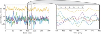
are all initialized to be the mean values of the joint limits so that the nominal trajectory is centered at the middle of the joint space with no motion. After this initialization, our trajectory generation algorithm actually produces motion which covers the entire robot joint space (see Fig. 4) so that our resulting calibration should be valid throughout. During each iteration (
 $j = 1, \dots, N_s$
), our algorithm will update the next
 $N_c$
columns of
 $C$
, (i.e. the matrix
 $C_j$
) given knowledge of all previously computed columns
 $C_0, C_1, \dots, C_{j - 1}$
.
The numerically planned robot trajectory for estimation of the parameters
 $\boldsymbol{{x}}$
in our particular robot/IMU setup. The joint space curves are defined by 1818 B-spline coefficients. By varying these coefficients, we generated trajectory plans that minimize posterior uncertainty of the parameters
 $\boldsymbol{{x}}$
for precise estimation. Solving this problem directly (27) was not feasible on our research PC; however, our sequential trajectory planning method (33) enabled solution of this large-scale, inequality-constrained, nonlinear optimization problem.

Because of B-splines’ local support (21), the columns
 $C_j$
only have effect on the interval
 $\Omega _{0_j} = \left[y_{d + 1 + N_c(j - 1)}, y_{2(d + 1) + N_c(j - 1) + N_c}\right]$
. We could consider the information about
 $\boldsymbol{{x}}$
that sampling on this interval would yield. However, some of the affect of
 $C_j$
overlaps into the interval affected by
 $C_{j + 1}$
which is not desirable for solving the trajectory sequentially. Therefore, we associate with
 $C_j$
the interval
 $\Omega _{0_j}$
excluding the next interval
 $\Omega _{0_{j + 1}}$
. Specifically, the interval that we associate with
 $C_j$
is
 \begin{equation} \Omega _j = \Omega _{0_j} - \Omega _{0_j} \cap \Omega _{0_{j + 1}} = [y_{d + 1 + N_c(j - 1)}, y_{d + 1 + N_c j}]. \end{equation}
Using the general results for recursively processing sets of measurements for estimation [Reference Maybeck45], (26) can be decomposed into
 \begin{equation} \Sigma _x = \left(\Sigma _{\hat{x}}^{-1} + \Sigma _0^{-1} + \Sigma _1^{-1} + \dots + \Sigma _{N_s}^{-1} + \Sigma _{N_s + 1}^{-1}\right)^{-1} \end{equation}
where the covariance of
 $\boldsymbol{{x}}$
associated with interval
 $\Omega _j$
is
 \begin{equation} \Sigma _j = \left(\left[\frac{\partial \boldsymbol{{e}}_{z_j}}{\partial \boldsymbol{{x}}}\right]^\intercal \Sigma _{z_j}^{-1} \frac{\partial \boldsymbol{{e}}_{z_j}}{\partial \boldsymbol{{x}}} \right)^{-1}. \end{equation}
Here,
 $\boldsymbol{{e}}_{z_j}$
is the vector obtained by stacking all of the
 $\boldsymbol{{e}}_{z_i}$
that happen to fall in the interval
 $\Omega _j$
;
 $\Sigma _{z_j}$
are all of the associated covariance matrices.
The covariances
 $\Sigma _j$
in (31) can be interpreted as the uncertainty of the parameters
 $\boldsymbol{{x}}$
, given only the data sampled within the interval
 $\Omega _j$
. In (30), all of these intervals are brought together with the prior covariance
 $\Sigma _{\hat{x}}$
to compute the posterior covariance
 $\Sigma _x$
.
Next, we note that we can truncate the sum in (30) after only a portion of the
 $N_s$
intervals have occurred. This suggests the following recurrence relationship to compute the posterior covariance of
 $\boldsymbol{{x}}$
after
 $j$
time intervals have occurred:
 \begin{equation} \Sigma _{x_j} = (\Sigma _{x_{j - 1}}^{-1} + \Sigma _j^{-1})^{-1} \end{equation}
where
 $\Sigma _{x_j}$
is the posterior covariance of
 $\boldsymbol{{x}}$
given measurements in all intervals up to and including
 $\Omega _j$
. The trajectory
 $\boldsymbol{{q}}(t)$
(and thus the data sampled) in
 $\Omega _j$
is only dependent on the coefficients
 $C_j$
due to the locality of B-splines. Thus, the covariance
 $\Sigma _j$
is only a function of
 $C_j$
, a small subset of the full parameter matrix
 $C$
. Further, the construction of
 $\Omega _j$
ensures that
 $C_j$
will have no effect on the prior covariance
 $\Sigma _{x_{j - 1}}$
which (given all
 $C_k$
where
 $1 \leq k \lt j$
) has already been established in the previous iteration.
Therefore, instead of solving the optimization problem (27) all at once, during each of the
 $N_s$
iterations, we instead solve the following local problem:
 \begin{equation} C_j^* = \underset{C_j}{\arg \min }\{\max \text{svd} (\Sigma _{x_j})\} \\ \end{equation}
subject to the same trajectory constraints (28) as the global problem. Solving (33) for
 $j = 1 \dots N_s$
will give all of the columns of the full matrix
 $C$
which should approximately solve (27).
During each iteration, this process can be thought of as adding onto the trajectory some new small trajectory piece over the added interval
 $\Omega _j$
. This additional trajectory piece only affects
 $\Sigma _j$
in the sum in (32). By changing
 $C_j$
, we design the information
 $\Sigma _j$
in this new interval to optimally combine with the prior, known information
 $\Sigma _{x_{j - 1}}$
from the previous iterations. Note that the B-spline function representation ensures that the function
 $\boldsymbol{{q}}(t)$
maintains continuity over its entire domain throughout this process.
This sequential approach may not lead to exactly the same solutions as directly solving (27); however, it is more practical. Furthermore, in our numerical experiments, trajectories generated in this way achieve parameter estimates that are 10 times more precise than using a random trajectory. Finally, because the approach essentially adds to the full trajectory a new small piece, it can be terminated once the covariance
 $\Sigma _x$
becomes sufficiently small which makes the method more flexible than solving (27) directly.
7.4. Full calibration pipeline
Here, we summarize the required steps to use our method to calibrate a robot/IMU pair. Below is a practical step-by-step guide explaining the general pipeline of our algorithm. Prior models for both the robot and the IMU are assumed.
-
1. Using the methods in Section 7, numerically generate a trajectory plan
 $\tilde{\boldsymbol{{q}}}$
. Note that any trajectory could be used in principle, but calibration results may be less accurate.
-
2. Command the physical robot/IMU setup to follow the desired trajectory
$\tilde{\boldsymbol{{q}}}$
. During motion, collect both robot joint position data
$\boldsymbol{{q}}_{1:N_q}$
and IMU sensor data
$\boldsymbol{{z}}_{1:N_z}$
. -
3. Given the observed data, set up and solve the nonlinear least-squares problem (22) for the vector of unknowns
$\boldsymbol{\theta } = [\boldsymbol{{x}}^\intercal \quad \boldsymbol{{c}}^\intercal ]^\intercal$
. Note that the posterior covariance for all parameters
$\Sigma _\theta$
can also be computed using (24).


Ultimately, the following sections perform these operations for an example robot/IMU pair and then validate the results using ground truth data from an optical tracker.
8. Numerical experiments
8.1. Nominal system parameters and prior uncertainties
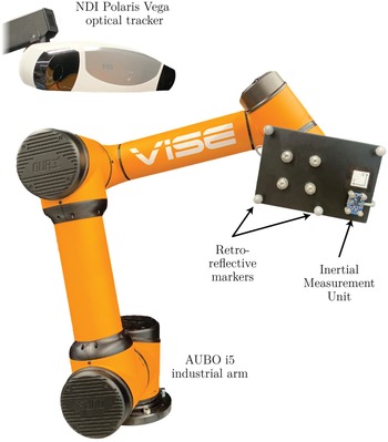
All of our numerical and real experiments are conducted with an AUBO i5 collaborative industrial arm (AUBO Robotics, USA) with an end-effector-mounted Bosch BNO055 9-axis orientation sensor (see Fig. 9). Note that while this IMU is capable of estimating some of its parameters online, throughout our experiments, we are using it in the raw output mode collecting only raw triaxial accelerometer and gyroscope outputs. Note that while these outputs are generally voltages, our IMU instead outputs in inertial units converting using hard-coded gain values internally. While this does affect the units of our identified and nominal parameters (e.g. unitless sensor gains, biases with non-voltage units), it does not affect our method, as these parameters can be formed into an equivalent model. Here, we justify all of the nominal parameters (and their prior uncertainties) related to our numerical and real experiments. A summary of this information is shown in Table II.
By definition, the nominal values for all of the robot kinematic errors
 $\boldsymbol{\epsilon }$
are zero, and as machining errors are generally on the order or 0.1 mm, we conservatively choose prior STDs of 1.0 mm for length parameters and 1.0
 $^\circ$
for angle parameters. Nominally, the gravity direction parameters
 $g_x$
and
 $g_y$
are zero as gravity should only be acting in the
 $Z$
axis, but if the robot is mounted on the table with some angle
 $\theta _0$
, then the largest that either could be is
 $9.81 \sin \theta _0.$
A conservative value for
 $\theta _0$
is
 $5^\circ$
; this implies a prior STD for
 $g_x$
and
 $g_y$
of about 0.5 m/s
 $^2$
. As we have no prior information about the time offset
 $\tau$
, its nominal value is zero, and we conservatively choose a large prior STD of 1 s. The IMU board was oriented carefully onto the end-effector at the nominal orientation for
 $\boldsymbol{{r}}_a$
and
 $\boldsymbol{{r}}_\omega$
. However, to account for potential mounting and machining errors, we choose prior STDs of 5
 $^\circ$
for the sensor orientations. The position of the IMU board relative to the end-effector was measured with a set of calipers; to account for measurement error here, we choose a prior STD of 10 mm for the parameters
 $\epsilon _{6_1}$
,
 $\epsilon _{6_2}$
, and
 $\epsilon _{6_3}$
.
The nominal values and prior uncertainties for the sensor parameters were chosen based on the IMU data sheet [46]. For the triaxial accelerometer, the maximum cross axis sensitivity was quoted to be 2%. This means that the maximum misalignment angle is
 $\sin ^{-1}(0.02) = 1.146^\circ$
, so we choose prior STDs of 1.5
 $^\circ$
for
 $\boldsymbol{\gamma }_a$
to be conservative. The maximum deviation of the accelerometer sensitivity was quoted to be 4%. Therefore, we conservatively choose prior STDs of 0.1 for
 $\boldsymbol{{k}}_a$
. The maximum zero-
 $g$
offset was quoted to be
 $150 \text{mg} = 1.4715 \text{m/s}^2$
, so we conservatively choose prior STDs of 2.0 m/s
 $^2$
for
 $\boldsymbol{{b}}_a$
. The gyroscope cross axis sensitivity was quoted to be 3%. Therefore, as
 $\sin ^{-1} (0.03) = 1.7191^\circ$
, we choose prior STDs of 2.0
 $^\circ$
for
 $\boldsymbol{\gamma }_\omega$
. The maximum deviation of the sensitivity was quoted to be 3%. Therefore, we choose prior STDs of 0.1 for
 $\boldsymbol{{k}}_\omega$
. The maximum zero-rate offset was quoted to be 3
 $^\circ$
/s. Given this, we choose prior STDs of 5
 $^\circ$
/s for
 $\boldsymbol{{b}}_\omega$
.
We adopt the standard assumption throughout our experiments that the parameters
 $\boldsymbol{{x}}$
are not initially correlated. Therefore, the initial covariance of the parameters
 $\Sigma _{\hat{x}}$
is diagonal; the elements on the diagonal of
 $\Sigma _{\hat{x}}$
are then the squares of the initial standard deviations in Table II.
Trajectory planning (33) and calibration of the system (22) both require knowledge of the covariance matrices
 $\Sigma _{z_j}$
associated with the IMU measurements. Here, we again apply the standard assumption that the measurements are not correlated. Additionally, we assume that the covariance is constant during robot motion – that is,
 $\Sigma _{z_1} = \ldots = \Sigma _{z_N} = \Sigma _z$
. While
 $\Sigma _z$
can be estimated by sampling the IMU under static conditions, in our experiments, we found the measurement noise to be significantly greater when the robot is moving. Therefore, to determine
 $\Sigma _z$
we moved the robot–IMU setup (Fig. 9) dynamically while sampling the IMU. The samples
 $\boldsymbol{{z}}$
, collected over 300 s, were then least-squares fit to a spline function (20). The errors between the fit and the data were then used to compute the covariance
 $\Sigma _z = \text{diag}[0.38^2 \quad 0.21^2 \quad 0.19^2 \quad 0.32^2 \quad 0.47^2 \quad 0.57^2]$
where the first three elements, corresponding to specific force variance, have units of (m/s
 $^2$
)
 $^2$
and the last three elements have units of (
 $^\circ$
/s)
 $^2$
and represent angular velocity variance. Using similar methods and assumptions, we determined the constant, diagonal covariance of the measured joint values to be
 $\Sigma _q = \text{diag}[0.0038^2 \quad 0.0050^2 \quad 0.0043^2 \quad 0.0105^2 \quad 0.0101^2 \quad 0.0086^2] (^\circ )^2$
.
8.2. Numerical trajectory planning
In order to proceed with any of our other experiments, first we must choose the planned trajectory for the robot to follow during data collection. Here, we discuss the details of implementing our trajectory planning method (Section 7) with our particular robot–IMU setup. After planning, we compare the performance of the planned trajectory to a random trajectory of the same length to determine the performance gain by using the optimal trajectory.
We generated a 300 s trajectory using our recursive method outlined in Section 7. To build the matrices in (31), we assumed a sample rate for the IMU and the joint values of 120 Hz as this was approximately the value achieved by our system. For the trajectory representation, we chose to use a spline of degree
 $d = 3$
with one interior knot per second. This leads to a
 $C$
having 303 columns in total. Taking into account the known padding blocks
 $C_0$
and
 $C_{N_s + 1}$
, this leads to 297 columns of
 $C$
to determine. We used a block size of
 $N_c = 5$
columns per iteration. Given our 6 axis robot model, this leads to solving (33) for
 $N_s = 60$
iterations to determine the unknown elements of
 $C$
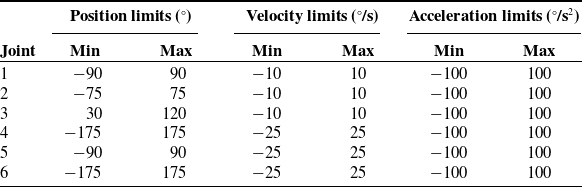
. In order to constrain the motion (28) within safe operating conditions, we used the joint limits shown in Table III.
Robot joint position, velocity, and acceleration limits for our experiments.

Note that these values are chosen conservatively to maintain safe operating trajectories.
During each iteration, we used a hybrid global optimization method to solve (33) for the 30 elements of
 $C_j^*$
. First, we ran 2000 iterations of the simulated annealing algorithm (implemented in MATLAB’s simulannealbnd function) to determine
 $C_j$
globally. This was followed by a local refinement step using the Hooke’s–Jeeves pattern search algorithm (as implemented in MATLAB’s patternsearch function) with 200 iterations, a maximum mesh size of 0.5, and compete polling. The optimal trajectory generated is shown in Fig. 4.
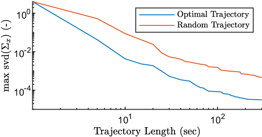
The trajectory performance measure (33) is shown decreasing with time in Fig. 5.
Identifiability of the robot–IMU system parameters versus trajectory length. Compared with a random trajectory of the same length, the planned trajectory generated by our sequential trajectory planning method reduced the identifiability measure by at least an order of magnitude.

Also shown here is the same identifiability measure computed using a random trajectory as opposed to the optimal trajectory. This random trajectory was determined by selecting uniformly random values for the matrix
 $C$
while still adhering to the trajectory constraints (28).
Additionally, using the relationship (32), we computed the posterior standard deviations (the square roots of the diagonals of
 $\Sigma _{x_j}$
) of all of the parameters in
 $\boldsymbol{{x}}$
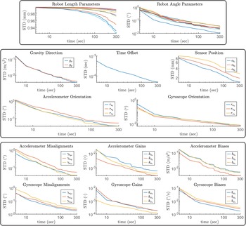
. These are plotted versus time in Fig. 6. To verify the approximation (26), we compared the approximate covariance
 $\Sigma _x$
to the covariance predicted by the estimator (24). After the full trajectory, the Frobenius norm between the two covariances was 4.7e-6.
Estimated posterior standard deviations of system parameters
 $\boldsymbol{{x}}$
versus optimal trajectory length. Top: robot kinematic error parameters
 $\boldsymbol{\epsilon }$
. Middle: extrinsic system parameters
 $\boldsymbol{{g}}_{xy}$
,
 $\tau$
,
 $\boldsymbol{{r}}_a$
, and
 $\boldsymbol{{r}}_\omega$
. Bottom: IMU sensor parameters
 $\boldsymbol{\gamma }_a$
,
 $\boldsymbol{{k}}_a$
,
 $\boldsymbol{{b}}_a$
,
 $\boldsymbol{\gamma }_\omega$
,
 $\boldsymbol{{k}}_\omega$
, and
 $\boldsymbol{{b}}_\omega$
. The estimation precision of all parameters improves with trajectory length for our particular system.

8.3. Monte Carlo simulations
To verify the identifiability of the parameters
 $\boldsymbol{\theta } = [\boldsymbol{{x}}^\intercal \quad \boldsymbol{{c}}^\intercal ]^\intercal$
under our assumptions, we performed a series of Monte Carlo simulations. In each of the simulations, data were generated using ground truth parameters, noise was injected into the data, and then (22) was solved using the noisy data to estimate the true parameters. In the following, we describe this process for a single iteration.
First, we sample the ground truth set of parameters using the nominal values and standard deviations shown in Table II. Next, using the optimal trajectory
 $C^*$
, the ground truth parameters, and the determined covariances
 $\Sigma _z$
and
 $\Sigma _q$
, we generate the required data
 $\boldsymbol{{q}}_i$
and
 $\boldsymbol{{z}}_i$
for
 $i = 1 \dots N$
with (10). Using these measurements along with the nominal parameters as an initial guess, we compute the estimate (22) and posterior covariance (24) of the parameters
 $\boldsymbol{\theta }$
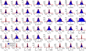
. This process was repeated for 100 simulations, and estimation errors for
 $\boldsymbol{{x}}$
are shown in Fig. 7.
Histograms of errors between the 48 estimated and ground truth system parameters
 $\boldsymbol{{x}}$
in our 100 Monte Carlo simulations. The red lines indicate the posterior distributions predicted by the estimator (i.e. Eq. (24)) which match closely with the histogram data.

8.4. Robot length parameter identifiability
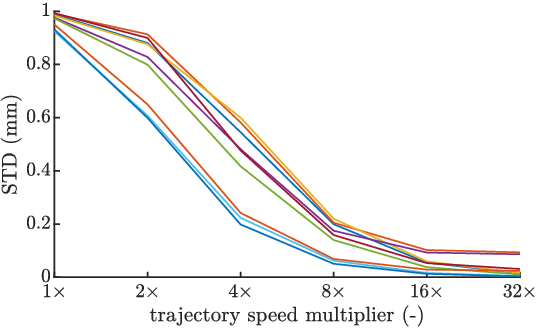
As discussed in Section 10, our numerical results indicate that for our particular setup, robot length parameters (e.g. link lengths) cannot be estimated with much certainty. We hypothesize that restrictions on robot joint speeds and accelerations (see Table III) could affect identifiability of robot length parameters. Here, we perform a numerical experiment analyzing the effect of trajectory speed on length parameter identifiability.
Our generated 300 s optimal trajectory was used to define several faster trajectories. This was done by scaling the
 $X-$
axis by different amounts so that the original trajectory was completed in less time. In this way, we created five new trajectories: one that was
 $2\times$
faster than the original, one
 $4\times$
, one
 $8\times$
, and so on. Using (26), the posterior standard deviations of the robot length parameters were computed for each of the different trajectory speeds. We adjusted the 120 Hz sample rate to achieve the same number of data samples for each trajectory (e.g. 240 Hz for the
 $2\times$
trajectory). Posterior uncertainty of robot length parameters is shown decreasing with trajectory speed in Fig. 8.
Predicted posterior standard deviations of the nine robot length parameters (e.g. link lengths) versus trajectory speed. As the speed of robot motion increases, the precision on length parameters improves substantially. While our robot’s motion was bounded by the values in Table III, faster robots could enjoy accurate length parameter calibration with our method.

9. Experimental results
To verify our method’s ability to increase robot accuracy and sensor accuracy, we performed a set of experiments testing our method with an AUBO i5 collaborative industrial arm with an end-effector-mounted Bosch BNO055 9-axis orientation sensor (see Fig. 9).
Additionally, we used an NDI Polaris Vega optical tracker (with a quoted accuracy of 0.12 mm) to measure the accuracy of the robot and the sensors. With the tracker, we also performed “standard” calibrations of both the robot and the IMU separately for comparison with our estimated values. Note that the optical tracker was used for verification purposes only.
The aluminum plate mounted to the end-effector flange served to hold the retro-reflective markers (for optical tracking) and the IMU board rigid with respect to the robot’s end-effector. The IMU reported its samples to an Arduino Mega microcontroller using the I
 $^2$
C digital communication protocol. Software was written to command the robot along the desired optimal trajectory. Additionally, separate data collection software was written to simultaneously record the robot’s joint values (via MATLAB’s ROS toolbox) and the IMU sensor readings (via MATLAB’S serial interface).
Experimental setup to test our calibration method’s ability to improve accuracy of the robot and sensor models. An aluminum plate with a Bosch BNO055 IMU and optical tracking spheres is mounted to the end-effector of an AUBO i5 industrial collaborative robot. The NDI Polaris Vega optical tracker is used for ground truth data acquisition only to evaluate our calibration method’s ability to improve robot and sensor accuracy.

The robot was first commanded along the optimal trajectory while recording its joint values and the sensor readings on a separate PC. This information was then used to infer
 $\boldsymbol{\theta }$
and thus the model parameters
 $\boldsymbol{{x}}$
using (22). The resulting values are shown alongside their nominal counterparts in Table II. Based on the results of our numerical experiments in Section 8, in our real experiments, we made the choice to exclude robot length parameters from the calibration. This was achieved by setting their prior covariances to small numbers so that they would not be updated by calibration. Therefore, only the updated robot angle parameters are shown in Table II. This limitation of our method is discussed thoroughly in Section 10. To test the convergence of the algorithm on experimental data, we additionally subdivided the full 5 min of data to perform five 1-min calibrations. The maximum differences between these five calibrations and the values in Table II were 0.36
 $^\circ$
for
 $\boldsymbol{\epsilon }$
, 0.036 m/s
 $^2$
for
 $\boldsymbol{{g}}_{xy}$
, 0.0029 s for
 $\tau$
, 0.30
 $^\circ$
for
 $\boldsymbol{\gamma }_a$
, 0.33
 $^\circ$
for
 $\boldsymbol{{r}}_a$
, 0.0028 for
 $\boldsymbol{{k}}_a$
, 0.0402 m/s
 $^2$
for
 $\boldsymbol{{b}}_a$
, 0.22
 $^\circ$
for
 $\boldsymbol{\gamma }_\omega$
, 0.0621
 $^\circ$
for
 $\boldsymbol{{r}}_\omega$
, 0.00082 for
 $\boldsymbol{{k}}_\omega$
, and 0.0158
 $^\circ$
/s for
 $\boldsymbol{{b}}_\omega$
.
Following the identification procedure, we began the robot accuracy evaluation process. The robot was next commanded to 250 discrete configurations for robot accuracy evaluation. Once at a configuration, the pose of the end-effector was sampled for 3 s. The poses at a particular configuration were then averaged using the quaternion-based rotation averaging algorithm [Reference Markley, Cheng, Crassidis and Oshman47].
To verify our method’s ability to identify robot parameters, we performed a standard robot calibration [Reference Meggiolaro and Dubowsky38] using 150 of the 250 collected poses. Note that because our method could not calibrate length parameters precisely in our setup, length parameters were also excluded in the standard calibration. The standard calibration values are shown alongside our calibration values in Table II. The constant transforms
 $T^{\text{tracker}}_{\text{robot}}$
and
 $T^{\text{markers}}_{\text{end effector}}$
necessary for evaluating robot accuracy were then extracted from the standard calibration.
To test our method’s ability to improve robot accuracy, the remaining 100 poses were used to compute accuracy using nominal parameters, our calibration parameters, and the standard calibration parameters. The positional accuracy was computed using the standard Euclidean norm between the tracker-measured and model-predicted end-effector positions. The rotational accuracy was taken as the standard minimal geodesic distance between the measured and predicted end-effector rotations,
 $R_{\text{meas}}$
and
 $R_{\text{pred}}$
. In other words, the rotation error is defined as the angle of the rotation
 $R_{\text{meas}}^\intercal R_{\text{pred}}$
. These robot translation and rotation accuracy results are shown in Fig. 10.
To verify our method’s ability to identify IMU parameters, we performed a standard IMU calibration [Reference Kim and Golnaraghi7] using the optical tracker. The setup was manipulated along a random 20 min trajectory while recording both tracker-based pose and raw IMU data. These data together were used for IMU calibration. Note that the angular parameters relative to the end-effector were not included in the standard IMU calibration which was relative to the tracked markers. The standard calibration values are shown alongside our calibration values in Table II.
In addition to improving the robot accuracy, our method should improve the accuracy of the IMU sensors. Immediately after running the optimal calibration trajectory, a different random 120 s trajectory was run to evaluate the accuracy of the IMU sensors. During this process, the pose of the end-effector was measured using the optical tracker for evaluation purposes. Given the alignment of the end-effector with the markers (known from the standard robot calibration above) and the alignment of the end-effector with the IMU (known from our calibration), the tracked pose of the IMU was computed. Splines of degree 5 and one interior knot per 30 samples were fit to the IMU position and quaternion data. These spline functions were differentiated to obtain ground truth IMU acceleration and angular velocity functions. The ground truth-specific force was then computed from the acceleration data using the estimated gravity direction vector from the calibration
 $\boldsymbol{{g}}_{xy}$
. In order to assess IMU calibration accuracy relative to the tracker data, the tracker must first be temporally aligned with the IMU. To accomplish this, first the tracker was temporally aligned with the robot data using a subset of the trajectory. Then the required tracker/IMU temporal alignment is just the sum of this tracker/robot alignment and the estimated robot/IMU alignment
 $\tau$
in Table II. Using the temporal offsets, the ground truth-specific forces and angular velocities were evaluated at the same time of the IMU samples and then transformed into the accelerometer and gyroscope coordinate systems, respectively.
Histograms showing both position and rotation robot accuracy before calibration (top), after our calibration (middle), and after a standard calibration (bottom). Accuracy is evaluated by comparing the model-predicted end-effector pose to the optically tracked ground truth. Note that neither our calibration nor the standard calibration includes length parameters.

The accelerometer and gyroscope IMU outputs were computed using the inverse of (6) using nominal sensor parameters and our calibration parameters, and the standard calibration parameters. The normed differences between the sensor outputs and the ground truth inertial quantities measured with the tracker are shown in Fig. 11 where we have applied a moving mean filter with a window size of 500 samples.
Histograms showing both specific force and angular velocity sensor accuracy before calibration (blue), after our calibration (red), and after a standard calibration (yellow). Accuracy is evaluated by comparing the sensor model-predicted values to the optically tracked ground truth. Note that data have been passed through a moving mean filter with a 500 sample window.

10. Discussion
In our numerical experiments (see Fig. 6), all of the parameters’ STDs were reduced by calibration, and the identification Jacobian was found to be full rank and well-conditioned over the calibration trajectory. Furthermore, our Monte Carlo simulations indicate that, given all assumptions about the system and associated noise profiles, our calibration converges to the correct values. This indicates that the IMU and joint angle measurements provide enough information to infer
 $\boldsymbol{{x}}$
in our setup.
While the robot angle parameter uncertainties were all reduced by at least a factor of 10, calibration only changed the robot length parameter uncertainties marginally (see Fig. 6). This suggests that, in our particular setup, calibration of the robot length parameters – while mathematically possible – is not practically feasible. For these reasons, we chose not to include the robot length parameters as calibration variables in our real experiments.
The identifiability of the robot length parameters could be improved with a longer trajectory; however, this comes with additional time and computation costs. As only the accelerometer measurements can give robot length parameter information, the lengths could be identified more accurately by improving the accelerometer signal to noise ratio. As mentioned previously, accelerometer noise was dominated by the vibrations of the system during trajectory following; therefore, we believe that using a higher fidelity IMU is unlikely to make a large difference. Instead, we propose that it is more practical to improve robot length parameter identifiability by utilizing faster robot trajectories. Our real experiments were limited to the motion constraints in Table III; however, our numerical experiments (Fig. 8) suggest that the identifiability of robot length parameters can be significantly improved with faster trajectories. Application of our method to high-speed robots for full Level II [Reference Roth, Mooring and Ravani1] calibration (both length and angle parameters) could be the basis for future work.
The problem proposed in this paper requires long robot trajectories in order to acquire enough information for a good calibration. Thus, we used trajectory planning to ensure information richness of the robot motion, ultimately enabling shorter trajectories. Traditionally, trajectory planning involves computing the entire optimal trajectory all at once [Reference Swevers, Ganseman, Tukel, De Schutter and Van Brussel42, Reference Park48–Reference Wilson, Schultz and Murphey50]. In our numerical experiments, this approach led to an inequality-constrained, nonlinear optimization problem in 1782 variables. Due to this size and complexity, solution of this trajectory optimization problem was not feasible on our research PC. Alternatively, our sequential approach to trajectory planning makes computation of such long trajectories feasible by splitting the large-scale problem into many simpler ones. As shown in Fig. 5, our trajectory planning method significantly improved the identifiability of the system parameters
 $\boldsymbol{{x}}$
. The optimal trajectory yielded a posterior covariance of
 $\boldsymbol{{x}}$
with a maximum singular value of 3.1e-05, whereas the random trajectory yielded a value of 4.6e-04. This implies that the posterior STDs are bounded by 0.0056 and 0.0215, respectively. Therefore, compared with a random trajectory, the optimal trajectory made the calibration 3.8 times more accurate for our system. We note that based on Fig. 5, adequate results are eventually possible with a random trajectory; however, in our experiments, an optimal trajectory is more efficient, achieving the same level of precision in less time.
Our Monte Carlo simulations (Fig. 7) validate our method given all assumptions about the system and the noise profiles of the sensors. Specifically, these results verify the approximation of
 $\Sigma _x$
in our trajectory planning method. As shown in Fig. 7, all of the predicted distributions based on the approximation (26) matched closely with the histograms output by the Monte Carlo simulations. Therefore, we can assume the approximation of
 $\Sigma _x$
(26) to be reasonably accurate for our system.
Our real experiments show that our method works in practice to identify robot angle parameters. In Table II, the average and maximum error between our identified angle parameters and the standard calibration was 0.04
 $^\circ$
and 0.09
 $^\circ$
, respectively. Our method also significantly improved robot accuracy. This is shown in Fig. 10 by the error reduction of both the position and rotation model predictions. Before calibration, the mean position accuracy was 1.58 mm; our calibration reduced this metric to 0.55 mm, near the 0.49 mm obtained by the standard calibration. Rotation accuracy was also improved by our method bringing the mean accuracy from 0.37
 $^\circ$
down to 0.13
 $^\circ$
, very near the 0.13
 $^\circ$
achieved by the standard calibration.
All of this suggests that our method is comparable to a standard robot calibration for estimating angle parameters. Thus, our approach offers a cheap and fast Level I robot calibration [Reference Roth, Mooring and Ravani1] (i.e. calibration of the joint angle offsets) as well as a partial Level II robot calibration (i.e. calibration of the entire rigid kinematics model). As previously noted, full Level II calibration could even be achieved given a sufficiently fast robot trajectory (see Fig. 8), but this was not possible in our specific setup. The incapability of the method to estimate link lengths in our specific setup is likely not a large concern as an accuracy of 0.55 mm is adequate for most applications. Furthermore, it has previously been shown that for industrial arms, the majority of positional error is actually caused by errors in joint angle offsets rather than the other kinematic parameters [Reference Shiakolas, Conrad and Yih51].
Another area of future work is in the application of these approaches to redundant and continuum robots. Sensing and calibration for redundant and infinite degree of freedom robots are an active area of research [Reference Modes and Burgner-Kahrs52]. We believe that IMUs could be used on these robots to calibrate parameters such as base frame parameters and material property constants, which is an exciting potential area for future work.
In addition to robot angle parameter calibration, our method also provides an IMU sensor calibration. All of our calibrated values match reasonably well with the standard IMU calibration in Table II. Our method also substantially improved the accuracy of the IMU sensors. Both angular velocity and specific force errors were reduced when compared to the optically tracked ground truths (see Fig. 11). Specifically, over the 60 s evaluation trajectory, the angular velocity errors were reduced from 2.17
 $^\circ$
/s to 0.95
 $^\circ$
/s in the RMS sense; the standard calibration also achieved 0.95
 $^\circ$
/s. For the accelerometers, specific force errors were reduced from 0.93 m/s
 $^2$
to 0.77 m/s
 $^2$
in the RMS sense; the standard calibration also achieved 0.77 m/s
 $^2$
.
All of this suggests that our method is comparable to a standard IMU calibration. Based on these results, and given that our method could be used with multiple IMUs at once, we believe that our method could be useful in cases where many IMU sensors need to be calibrated quickly such as in a sensor manufacturing facility.
Finally, based on our Monte Carlo simulation, our method also accurately estimates all of the extrinsic parameters of the IMU (i.e. spatial offset, temporal offset, and gravity). This makes our method ideal as an initial calibration step enabling the use of IMU data in online robot estimation and monitoring applications.
11. Conclusion
In this work, we proposed and evaluated a new method for jointly estimating robot kinematic parameters, inertial sensor parameters, and various extrinsic parameters relating the two (spatial offsets, temporal offsets, and gravity). Enabled by recent advancements in continuous-time batch trajectory estimation, we showed that the MAP estimate leads to a nonlinear least-squares problem and derived the sparsity structure of the associated Jacobian. Additionally, as long robot trajectories were required to achieve a good calibration, we proposed a new method to generate trajectory plans sequentially, building the trajectory piece-by-piece. In our specific application, our results suggest that it achieves estimates that were many times more precise than a random trajectory. Note that generalization of our sequential trajectory planning approach to many other estimation scenarios (e.g. robot dynamic identification [Reference Swevers, Ganseman, Tukel, De Schutter and Van Brussel42, Reference Park48]) is straightforward. Using this optimal trajectory, we evaluated our approach in a Monte Carlo simulation showing that the calibration produces the correct result on average. Our numerical results also suggest a strong link between trajectory speed and robot length parameter identifiability. While length parameters could not be accurately estimated in our particular setup, application of our method to high-speed robots for full kinematic calibration could be the basis of future work.
Our method improved the accuracy of the robot in our experiments substantially, suggesting a potential application in Level I robot calibration (i.e. determining joint angle offsets) as well as a partial Level II robot calibration (i.e. calibration of the entire rigid kinematics model) [Reference Roth, Mooring and Ravani1]. Furthermore, the method significantly reduced inertial sensor errors when compared to a ground truth showing promise for an alternative method of IMU sensor calibration. Our experiments show that our method is comparable to standard methods for robot and IMU calibration. Based on our Monte Carlo simulation, our method also accurately estimated the extrinsic parameters of the IMU (i.e. the IMU translation, rotation, and temporal offset relative to the robot). This makes our method ideal as an initial calibration step enabling the use of IMU data in online robot estimation and monitoring applications.
Author contributions
JMF conceived and designed the study. TEE and JMF conducted data gathering. JMF, TEE, and RJW wrote the article. SDH and RJW provided practical feedback and guidance throughout the study.
Financial support
This research was supported by National Institutes of Health under grant R01-EB023717. The content is solely the responsibility of the authors and does not necessarily represent the official views of the National Institutes of Health.
Conflicts of interest
The authors declare no conflicts of interest exist.
Ethical approval
Not applicable.