1. Introduction
The present work is an attempt to design an effective control mechanism for turbulent plane Couette flow. Controlling turbulent flows is a matter of significant scientific and societal interest, but one that is made difficult by the enormous complexity of turbulence dynamics. This complexity has motivated the development of reduced-order models (ROMs) that capture essential turbulence traits. Here, we explore such a ROM for Couette flow, using it to optimise a body forcing that laminarises the flow. The underlying turbulence suppression mechanism is then studied in the ROM and in the full Navier–Stokes system using direct numerical simulation (DNS). We start with a literature review which is organised in three main topics: Couette flow (§ 1.1), ROMs (§ 1.2) and turbulence control (§ 1.3). In § 1.4 we explain how these three topics are combined in the present study.
1.1. Couette flow
The present work focuses on plane Couette flow, a canonical configuration characterised by the relative motion of two parallel flat plates in the absence of a mean pressure gradient. In an ideal setting the plates are infinite, and the flow is homogeneous in the wall-parallel directions; consequently, the total shear stress is constant across the space between the plates. This makes plane Couette flow perhaps the simplest configuration, at least conceptually, for the study of wall-bounded turbulence.
Despite this apparent simplicity, Couette flow is quite challenging to execute experimentally, and relatively few experimental studies have been conducted with respect to other canonical configurations such as Poiseuille and pipe flows. Among important early experimental studies are, for instance, those of Reichardt (Reference Reichardt1956), Leutheusser & Chu (Reference Leutheusser and Chu1971) and El Telbany & Reynolds (Reference El Telbany and Reynolds1980). Some of the early experiments focused on the appearance of turbulent spots and on the onset of turbulence. Leutheusser & Chu (Reference Leutheusser and Chu1971) suggested a transitional Reynolds number of
 $Re_t \approx 300$
, based on the channel half-height and half the velocity difference between the walls. Other studies indicated slightly higher values of
 $Re_t$
. For instance, Malerud, Måløy & Goldburg (Reference Malerud, Måløy and Goldburg1995) suggested
 $Re_t = 370 \pm 10$
, whereas Tillmark & Alfredsson (Reference Tillmark and Alfredsson1992) and Daviaud, Hegseth & Bergé (Reference Daviaud, Hegseth and Bergé1992) proposed
 $Re_t \approx 360$
and
 $Re_t \approx 370$
, respectively. Later, through a series of extensive experiments with carefully controlled artificial excitation, Bottin et al. (Reference Bottin, Dauchot and Daviaud1997, Reference Bottin, Dauchot, Daviaud and Manneville1998) arrived at the more precise value of
 $Re_t=325$
. Later, other experimental studies have focused more on statistical properties of the flow in the fully turbulent regime and/or on the onset of large-scale coherent structures (Tillmark & Alfredsson Reference Tillmark and Alfredsson1998; Kitoh, Nakabyashi & Nishimura Reference Kitoh, Nakabyashi and Nishimura2005; Kitoh & Umeki Reference Kitoh and Umeki2008).
Given the limited amount of experimental data available, simulations have been widely used to study turbulence dynamics in plane Couette flow. The first DNS of turbulent plane Couette flow were performed by Lee & Kim (Reference Lee and Kim1991) at a friction Reynolds number of
 $Re_{\tau }=170$
(corresponding to
 $Re=3000$
based on the wall velocity and channel half-height) in a domain with dimensions of
 $4\pi h \times 8/3\pi h$
, with
 $h$
the half-channel height. More recently, advancements in computational power have enabled simulations at much higher Reynolds numbers and larger domains. For instance, Tsukahara, Kawamura & Shingai (Reference Tsukahara, Kawamura and Shingai2006), Avsarkisov et al. (Reference Avsarkisov, Hoyas, Oberlack and García-Galache2014), Pirozzoli, Bernardini & Orlandi (Reference Pirozzoli, Bernardini and Orlandi2014), Orlandi, Bernardini & Pirozzoli (Reference Orlandi, Bernardini and Pirozzoli2015) and Lee & Moser (Reference Lee and Moser2018) have performed simulations at Reynolds numbers and domain dimensions of
 $Re_{\tau }=126 (64h \times 6h)$
,
 $Re_{\tau }=550 (20\pi h \times 6\pi h)$
,
 $Re_{\tau }=986 (18\pi h \times 8\pi h)$
,
 $Re_{\tau }=986 (18\pi h \times 8\pi h)$
and
 $Re_{\tau }=500 (100\pi h \times 5\pi h)$
, respectively.
One of the most characteristic features of turbulence in Couette flow (and one that is shared by other canonical wall-bounded flows) is the presence of coherent streamwise streaks in the viscous and buffer layers. These streaks are organised in a pattern with a typical spanwise wavelength of
 $\lambda _z^+=100$
(Kline et al. Reference Kline, Reynolds, Schraub and Runstadler1967) in wall units. They interact with streamwise vortices in a cyclic process in which these structures are amplified, broken down and regenerated. This turbulence regeneration mechanism was first clearly identified by Hamilton, Kim & Waleffe (Reference Hamilton, Kim and Waleffe1995) in DNS of Couette flow in a small computational domain. Waleffe (Reference Waleffe1995, Reference Waleffe1997) further dissected this mechanism using ROMs and proposed that it is composed of three main processes: the amplification of streaks by streamwise vortices via the lift-up mechanism; the breakdown of streaks due to a secondary instability; and the nonlinear regeneration of streamwise vortices following the streak breakdown. This cyclic mechanism has since become known as a ‘self-sustaining process’ and is now widely recognised as a building block of wall turbulence. These processes also exist at much large scales. Streaky structures in the outer part of the flow, scaling with
 $h$
, are also amplified by the sheared mean flow (Hwang & Cossu Reference Hwang and Cossu2010a
) via transient growth, and it has been shown that these large-scale motions possess their own self-sustaining processes independent of those that occur in the buffer layer (Rawat et al. Reference Rawat, Cossu, Hwang and Rincon2015).
One trait that is particular to Couette flow is the existence of very-large-scale motions that occupy the entire length of the domain. Their signature starts to appear in domains larger than
 $5h$
in the spanwise direction (Tsukahara et al. Reference Tsukahara, Kawamura and Shingai2006; Kitoh & Umeki Reference Kitoh and Umeki2008; Avsarkisov et al. Reference Avsarkisov, Hoyas, Oberlack and García-Galache2014; Pirozzoli et al. Reference Pirozzoli, Bernardini and Orlandi2014; Orlandi et al. Reference Orlandi, Bernardini and Pirozzoli2015), and they can contribute to as much as half of the total shear stresses in the outer part of the flow (Pirozzoli et al. Reference Pirozzoli, Bernardini and Orlandi2014), their importance increasing with Reynolds number. The full spatial extent of such structures is only evident in very long domains. They were found to be correlated across domains as long as
 $100 \pi h$
in the streamwise direction (Lee & Moser Reference Lee and Moser2018), eventually becoming infinitely long at high Reynolds numbers.
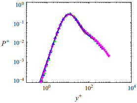
Despite the importance of these very-large-scale motions in the outer region, their effect in near-wall turbulence is rather limited. They do produce some modulation of smaller-scale turbulence, increasing its intermittency (Pirozzoli et al. Reference Pirozzoli, Bernardini and Orlandi2014); however, turbulence production and dissipation rates of Couette flow are found to be remarkably similar in the near-wall region (viscous and buffer layers) across a range of Reynolds numbers. In fact, near perfect collapse of production and dissipation (when pre-multiplied and expressed in wall units) is already observed at moderate friction Reynolds numbers (
 $Re_{\tau } \leqslant 1000$
) in the near-wall region, as observed by Orlandi et al. (Reference Orlandi, Bernardini and Pirozzoli2015). This led the authors to suggest that Couette flow can be interpreted as an extreme case towards which Poiseuille flow tends in the limit of high Reynolds numbers.
1.2. Reduced-order models
Perhaps the most well-known technique to derive ROMs is Galerkin projection. This approach consists in projecting the governing (partial differential) equations onto a basis formed by a reduced number of spatial modes representing highly energetic and/or coherent flow structures. Reduced-order models can provide a useful framework in which to analyse nonlinear interactions between different structures, while conveniently keeping the number of interactions to a manageable size. In this spirit, Waleffe (Reference Waleffe1997) proposed a 4-mode model for a wall-bounded flow forced by a streamwise body force (which has become known in the literature as Waleffe flow), which allows discretisation using Fourier modes. The ROM describes important aspects of the nonlinear dynamics involving streaks and streamwise vortices, essential pieces of the intermittent regeneration cycle at the core of self-sustaining turbulent processes; however, it cannot sustain a chaotic regime. Larger models were proposed later, such as those by Eckhardt & Mersmann (Reference Eckhardt and Mersmann1999) (19 modes) and Moehlis, Faisst & Eckhardt (Reference Moehlis, Faisst and Eckhardt2004) (9 modes) for Couette and Waleffe flow, respectively. These models were built using Fourier modes as basis functions, and the simulations were found to lead to a chaotic behaviour. One important drawback of these ROMs, however, is that the typical turbulence lifetimes are much shorter than those observed in simulations of the full system, due to the model truncation. More recently, it was shown by Cavalieri (Reference Cavalieri2021) that turbulence lifetimes can substantially increase if the basis describes interactions between streamwise vortices and streaks of different spanwise wavelengths.
Proper orthogonal decomposition (POD) modes are a popular choice of basis functions (Aubry et al. Reference Aubry, Holmes, Lumley and Stone1988; Noack et al. Reference Noack, Afanasiev, Morzyński, Tadmor and Thiele2003; Khoo, Chan & Hwang Reference Khoo, Chan and Hwang2022), given that they optimally represent a given flow in terms of its energy. However, for large bases, higher-order modes may easily suffer from lack of convergence, as obtaining a large number of POD modes for a turbulent flow from experiments or simulations requires a significant amount of temporal data, which are necessary to converge two-point statistics. In order to circumvent this issue, a recent model developed by Cavalieri & Nogueira (Reference Cavalieri and Nogueira2022) for Couette flow considered a basis consisting of eigenfunctions of the controllability Gramian, computed from the linearised Navier–Stokes operator forced stochastically. For a linear system forced with white noise, these modes are equivalent to POD modes (Farrell & Ioannou Reference Farrell and Ioannou1993b ); but computing them from first principles, through the linearised operator, bypasses the convergence issue, with the additional advantage that no data (apart from the laminar solution) are required. The model is found to reproduce key turbulence statistics with reasonable accuracy and to display all features of scale interactions. It was later shown to be a useful tool to search for invariant solutions in plane Couette flow (McCormack, Cavalieri & Hwang Reference McCormack, Cavalieri and Hwang2024) and to explore generalised quasilinear approximations (Maia & Cavalieri Reference Maia and Cavalieri2024).
1.3. Turbulence control
A large part of the energy consumption in industrial and commercial activities worldwide is due to skin-friction drag when moving fluids along pipes and channels, and vehicles through fluid media. This has motivated the development of a great variety of strategies over the years to either reduce turbulent drag or to suppress turbulence altogether in wall-bounded flows. A large part of this effort has been directed towards pipe flows, channel flows and boundary layers, which are easier to implement experimentally than Couette flow. However, successful control strategies usually act by interfering with physical mechanisms that are common to all wall-bounded turbulent flows, which makes them relevant for the present work. Therefore, in the following we review a few of the most important control methods developed heretofore.
Control strategies can rely on passive techniques, which include, for instance, the use of geometric protrusions or roughness elements at the walls, such as riblets (Sirovich & Karlsson Reference Sirovich and Karlsson1997; García-Mayoral & Jiménez Reference García-Mayoral and Jiménez2011) and the use of hydrophobic surfaces (Min & Kim Reference Min and Kim2004; Aghdam & Ricco Reference Aghdam and Ricco2016). Active control techniques, relying on external excitation of the flow, have also been extensively explored. These techniques can be further broken down into open-loop and feedback approaches. Active feedback approaches have been designed using linear control theory. Early applications of control theory to fluid systems include the numerical works of Moin & Bewley (Reference Moin and Bewley1994) and Joshi, Speyer & Kim (Reference Joshi, Speyer and Kim1997), who controlled turbulent channel flows using full-state information, Högberg et al. (Reference Högberg, Bewley and Henningson2003), who implemented partial-state information control of a transitional channel flow and Chevalier et al. (Reference Chevalier, Hoepffner, Åkervik and Henningson2007), who controlled spatially growing boundary layers. Feedback methods usually require knowledge of a large portion of the turbulent velocity field, which limits their application in high-Reynolds-number flows and/or experiments, because the number of degrees of freedom (DoFs) of the system becomes prohibitively high. This difficulty has prompted the search for control schemes which use a relatively small amount of state information, usually supported by ad hoc assumptions. One example is the technique called ‘opposition control’ (Choi, Moin & Kim Reference Choi, Moin and Kim1994), wherein velocity fluctuations (usually in the wall-normal direction) are imposed at the wall in phase opposition to velocities measured by sensors positioned at some prescribed position
 $y_{s}$
away from the wall. The optimal sensor location is found to be close to
 $y_s^+=10$
, where the
 $^{+}$
superscript denotes inner (viscous) units. The technique is found to affect the dynamics of coherent structures in the form of streamwise vortices, and skin-friction reductions as large as 25 % were reported for channel flow at Reynolds number
 $Re=1800$
. One drawback of the technique is that in experimental applications it is impractical to measure instantaneous velocities away from the wall. This issue has been addressed in a recent study by Park & Choi (Reference Park and Choi2020), who showed that, using convolutional neural networks, it is possible to estimate wall-normal velocities at
 $y^+=10$
through wall measurements (which are more accessible in experiments) with good accuracy.
A quite popular open-loop drag-reduction technique is based on spanwise forcing of the flow, which can be achieved by an oscillating wall or by a body force localised in the vicinity of the wall. Reviews of different variants of this technique were made by Quadrio (Reference Quadrio2011) and, more recently, by Ricco, Skote & Leschziner (Reference Ricco, Skote and Leschziner2021); the latter provides a comprehensive account of existing numerical and experimental applications, as well as a detailed discussion on the underlying physical mechanisms. This approach has the merit of being realisable in experiments, as demonstrated, for instance, by Auteri et al. (Reference Auteri, Baron, Belan, Campanardi and Quadrio2010). They have designed a pipe flow experiment wherein the pipe is divided into several subsections allowed to rotate independently in the azimuthal direction. Different rotation speeds were set at each section, inducing a streamwise variation of the transverse velocity. The choice of forcing parameters (streamwise wavenumber, angular velocity and amplitudes) was guided by the parametric study carried out by Quadrio, Ricco & Viotti (Reference Quadrio, Ricco and Viotti2009) in DNS. Large turbulent drag reductions, of the order of 33 %, are achieved in the experiments at a friction Reynolds number of
 $Re_\tau = 200$
. More recently, Marusic et al. (Reference Marusic, Chandran, Rouhi, Fu, Wine, Holloway, Chung and Smits2021) have shown in experiments that if the actuation frequency is synchronised with that of large-scale structures that dominate the flow far from the wall, significant drag reductions can be achieved at very high friction Reynolds numbers (
 $Re_\tau = 12\,800$
). Although developed initially for channel flows, opposition control and spanwise wall motion are also effective in reduction skin friction in Couette flows, as shown by Ibrahim et al. (Reference Ibrahim, Yang, Doohan and Hwang2019) and Bengana et al. (Reference Bengana, Yang, Tu and Hwang2022), respectively.
Important reductions in skin-friction drag can, therefore, be obtained through opposition control and spanwise forcing in the turbulent regime, offering the possibility to achieve significant energy savings. An even more ambitious goal, however, is to attain complete laminarisation of the flow. This has been accomplished recently in a series of experiments by Kühnen et al. (Reference Kühnen, Song, Scarselli, Budanur, Burak, Riedl, Willis, Avila and Hof2018b
) and Kühnen et al. (Reference Kühnen, Scarselli, Schaner and Hof2018a
). In Kühnen et al. (Reference Kühnen, Song, Scarselli, Budanur, Burak, Riedl, Willis, Avila and Hof2018b
) four control methods in turbulent pipe flows with Reynolds numbers
 $Re=3100$
and
 $Re=5000$
were discussed: (i) vigorously stirring with four rotors located inside the pipe 50 diameters downstream of the inlet; (ii) flow injection in the wall-normal direction; (iii) flow injection parallel to the wall; (iv) local changes in the boundary conditions by impulsive acceleration of a pipe segment. The four methods lead to impressive reductions of friction losses, followed by complete disruption of turbulence and subsequent return to the laminar state. Somewhat counterintuitively, laminarisation is preceded by a transient increase of cross-stream velocity fluctuations and/or wall shear stresses. In Kühnen et al. (Reference Kühnen, Scarselli, Schaner and Hof2018a
) laminarisation is also achieved at Reynolds numbers up to
 $Re=6000$
using a passive device consisting of an obstacle that partially blocks the flow. Common to all of these approaches is the fact that in the controlled flow the mean turbulent velocity profile is flattened around the pipe centre. The flattened profiles are characterised by reduced levels of linear transient growth, which affects the non-modal amplification of large-scale streaks and rolls involved in the so-called self-sustaining processes (Hamilton et al. Reference Hamilton, Kim and Waleffe1995). Kühnen et al. (Reference Kühnen, Song, Scarselli, Budanur, Burak, Riedl, Willis, Avila and Hof2018b
) modelled these control methods in DNS by means of a body force that induces a velocity profile similar to that observed in the experiments. With this strategy they were able to achieve laminarisation in their simulations for Reynolds number up to
 $Re=10^5$
, thus confirming the link between flattening of the velocity profile and suppression of turbulence. A similar control mechanism was investigated by Hof et al. (Reference Hof, Lozar, Avila, Tu and Schneider2010) at lower Reynolds numbers characteristic of the transitional regime,
 $Re \lesssim 2300$
. At these Reynolds numbers, turbulence is spatially intermittent and takes the form of localised ‘puffs’ of disorganised motion (Barkley Reference Barkley2016). The shapes of the rear laminar–turbulent interface of the puffs were manipulated in DNS by means of a localised force moving with the puffs, producing a plug-like velocity profile. The results showed that, when this forcing is active over a short section of the pipe, it leads to a complete disruption of the turbulent puff. This was subsequently reproduced in pipe and channel flow experiments at
 $Re=2000$
, wherein the velocity profile at the rear end of the puff was distorted by the injection of a second turbulent puff upstream, mimicking the effect of the body forcing.
1.4. Using ROMs to design a turbulence control method
The above discussion illustrates the significant advancements that have been made in the field of turbulence control, followed by a deeper understanding of fundamental turbulence dynamics, via carefully designed experiments, DNS or a combination of both. In this work, we test an alternative route to devise a control strategy: we explore ROMs based on Galerkin projections.
It is now well-established that the Couette flow ROM of Cavalieri & Nogueira (Reference Cavalieri and Nogueira2022) reproduces many important aspects of turbulence dynamics, so a natural question arises: Can we use it to design effective turbulence control mechanisms? Given the high-dimensionality of fluid systems, control of the full state, even in linear systems, is often impractical in experimental and numerical applications. Therefore, the design of affordable control schemes using reduced-order representations of the state has been one of the major avenues explored by the flow control community (Bagheri et al. Reference Bagheri, Henningson, Hoepffner and Schmid2009; Noack, Morzynski & Tadmor Reference Noack, Morzynski and Tadmor2011; Rowley & Dawson Reference Rowley and Dawson2017). This has led to success cases of flow control using ROMs. Perhaps the most prominent examples are the stabilisation of cylinder wakes (Noack et al. Reference Noack, Afanasiev, Morzyński, Tadmor and Thiele2004a ,Reference Noack, Morzynski and Tadmor b ; Tadmor & Noack Reference Tadmor and Noack2004; Bergmann, Cordier & Brancher Reference Bergmann, Cordier and Brancher2005; Bergmann & Cordier Reference Bergmann and Cordier2008) and the attenuation of cavity oscillations (Rowley & Juttijudata Reference Rowley and Juttijudata2004; Rowley, Juttijudata & Williams Reference Rowley, Juttijudata and Williams2005; Cabell et al. Reference Cabell, Kegerise, Cox and Gibbs2006; Barbagallo, Sipp & Schmid Reference Barbagallo, Sipp and Schmid2009; Ahuja & Rowley Reference Ahuja and Rowley2010). However, control applications using Galerkin-based ROMs have been restricted, so far, to transitional flows and/or configurations where strong modal instabilities are present, which are characterised by periodic or quasi-periodic oscillations. Turbulence control is, to the best of our knowledge, less explored within the ROM framework. Serious doubts have been cast on the possibility of using ROMs to perform control for more challenging scenarios (Noack et al. Reference Noack, Morzynski and Tadmor2011). These doubts are often associated with inherent inconsistencies attributed to Galerkin models: a number of studies have raised the necessity of supplementing the ROM formulation with closure models (Aubry et al. Reference Aubry, Holmes, Lumley and Stone1988; Grimberg, Farhat & Youkilis Reference Grimberg, Farhat and Youkilis2020; Ahmed et al. Reference Ahmed, Pawar, San, Rasheed, Iliescu and Noack2021; Callaham, Brunton & Loiseau Reference Callaham, Brunton and Loiseau2022) or calibrating the modal basis (Cordier, Majd & Favier Reference Cordier, El Majd and Favier2010). The goal of these approaches is twofold: approximate the effect of unresolved scales, improving the accuracy of the models, and preventing numerical instabilities. However, the work of Cavalieri & Nogueira (Reference Cavalieri and Nogueira2022) has shown that robust ROMs for wall-bounded flows can be developed without the need for closure models. The level of truncation of their model can be increased arbitrarily, with no sign of numerical instabilities.
In light of this, here we explore the model by Cavalieri & Nogueira (Reference Cavalieri and Nogueira2022), modified with the addition of a steady body force, aiming at suppressing near-wall turbulence in plane Couette flow. As will be explained briefly, an optimal structure of the forcing is sought that minimises a functional representing the total fluctuation energy of the flow. The remainder or the paper is organised as follows: in § 2, the mathematical formulation of the model and the optimisation algorithm are discussed; § 3 presents the results of controlled flows at different Reynolds numbers and analyses of the underlying control mechanism; in § 4 we discuss the application of the forcing term optimised with the ROMs in the full system, through DNS; in § 5 we discuss some features of the control mechanism derived here in light of previous successful control approaches, followed by concluding remarks in § 6.
2. Reduced-order models
We study incompressible plane Couette flow with zero pressure gradient in Cartesian coordinates. The streamwise, wall-normal and spanwise directions are denoted by
 $(x,y,z)$
, respectively, and velocity components along these directions are denoted by
 $u$
,
 $v$
and
 $w$
. The flow is doubly periodic in the streamwise and spanwise directions, and the domain is a box with dimensions
 $L_x = 2\pi h$
,
 $L_z = \pi h$
along the streamwise and spanwise directions, respectively, where
 $h$
is the channel half-height. The walls move in opposite directions with velocities
 $\pm U_w$
. The Reynolds-number range considered in the present work is
 $Re= 1000{-}3000$
, corresponding to friction Reynolds numbers of
 $Re_{\tau }=66{-}170$
.
The Reynolds numbers and domain dimensions explored in this study are small compared with recent numerical studies on Couette flow (Tsukahara et al. Reference Tsukahara, Kawamura and Shingai2006; Avsarkisov et al. Reference Avsarkisov, Hoyas, Oberlack and García-Galache2014; Pirozzoli et al. Reference Pirozzoli, Bernardini and Orlandi2014; Orlandi et al. Reference Orlandi, Bernardini and Pirozzoli2015; Lee & Moser Reference Lee and Moser2018). One drawback of working with a small domain is that it prevents the formation of the so-called ‘extreme-scale motions’ (Lee & Moser Reference Lee and Moser2018). These structures have spanwise wavelength of approximately
 $\lambda _z =5h$
and remain correlated over the entire streamwise length of the domain. They are found to be responsible for a significant portion of the turbulent fluctuation energy in the outer region, and their importance grow with increasing Reynolds number. Capturing the signature of these structures, at least partially, requires a domain of spanwise length
 $L_z \geqslant 5h$
, which is not case in the present study (except in the DNS case C3_LargeBox, discussed in section § 4). The control mechanism discussed herein, therefore, focuses only on the dynamics of near-wall turbulence, i.e. the inner layer. As will be shown shortly, despite the small domain and low Reynolds numbers explored here, the flow dynamics in the near-wall region is quite consistent with that observed at much higher Reynolds numbers and domain sizes.
In the formulation presented in the following, velocities, spatial coordinates and time are made non-dimensional using the wall velocity and the channel half-height. The origin of the coordinate system is placed at the channel centre, and the walls are located at
 $y \pm 1$
. The flow geometry is depicted in figure 1.
Schematic of the flow geometry. The black curve represents the turbulent mean-flow profile. The red curve illustrates a generic body forcing term, whose radial structure is optimised following the method described in § 2.1. Here,
 $U_w$
is the wall velocity and
 $(x,y,z)$
correspond to the streamwise, wall-normal and spanwise directions, respectively.

The governing equations are the Navier–Stokes equations for velocity fluctuations around the laminar flow solution,
 $\textbf{u}_0 = [y \ 0 \ 0]^T$
 \begin{equation} \frac {\partial {\textbf{u}}}{\partial t} + ({\textbf{u}}_0 \cdot \nabla){\textbf{u}} + ({\textbf{u}} \cdot \nabla){\textbf{u}}_0 + ({\textbf{u}} \cdot \nabla){\textbf{u}} = -\nabla p + \frac {1}{\textit{Re}}\nabla ^2{\textbf{u}}, \end{equation}
where
 $p$
is the pressure and
 $Re$
is the Reynolds number based on the wall velocity and the channel half-height,
 $Re= U_wh/\nu$
, with
 $\nu$
the fluid kinematic viscosity. No-slip and no-penetration boundary conditions are imposed at the walls,
 $y=\pm 1$
, for the fluctuations. Velocity fluctuations are subject to the following modal decomposition:
 \begin{equation} {\textbf{u}}(x,y,z,t) = \sum _ja_j(t)\phi _j(x,y,z), \end{equation}
where
 $a_j$
are temporal coefficients. The modes,
 $\phi _j(x,y,z)$
, form an orthonormal basis, and each mode individually satisfies the continuity equation and the boundary conditions. Here, we use a modal basis composed of eigenfunctions of the controllability Gramian. These modes represent flow states that are most easily influenced by an external excitation in a linearised framework and the controllability Gramian corresponds to the covariance matrix for linear systems forced with space–time white noise (Farrell & Ioannou Reference Farrell and Ioannou1993a
,Reference Farrell and Ioannou
b
). The modes are therefore obtained from the linearised Navier–Stokes system, with linearisation performed about the Couette laminar flow solution, subject to white-noise forcing, as described in detail by Jovanović & Bamieh (Reference Jovanović and Bamieh2005). The approach takes advantage of the homogeneity of the flow in the streamwise and spanwise directions and combines the controllability modes with a normal mode ansatz for the basis
 \begin{equation} \phi _i(x,y,z) = \hat {\phi _i}(y)e^{\textrm{i}(k_xx + k_zz)},\end{equation}
where the streamwise and spanwise wavenumbers,
 $k_x$
and
 $k_z$
, are integer multiples of the fundamental wavenumbers,
 $\alpha = 2\pi /L_x$
,
 $\beta = 2\pi /L_z$
, respectively. The controllability modes,
 $\hat {\phi _j}$
are obtained through spectral methods, using a Chebyshev discretisation. These modes, as computed from the linearised Navier–Stokes equations, are complex valued. In order to deal only with real modes, we adopt the same strategy as in Cavalieri & Nogueira (Reference Cavalieri and Nogueira2022): we take separate modes for the real and imaginary parts of each
 $\phi _i$
, which leads to a pair of modes that only differ by a phase shift of
 $\pi /2$
. We consider a model that includes combinations of streamwise wavenumbers
 $k_x/\alpha = 0,1,2$
and spanwise wavenumbers
 $k_z/\beta = -2,-1,0,1,2$
. For the mean-flow modes,
 $k_x = k_z = 0$
, the linearised operator becomes singular (Jovanović & Bamieh Reference Jovanović and Bamieh2005), and in this case the modes are obtained through eigendecomposition of the linear operator for a viscous diffusion problem (Waleffe Reference Waleffe1997; Cavalieri & Nogueira Reference Cavalieri and Nogueira2022). The eigenfunctions of such problem are known as Stokes modes.
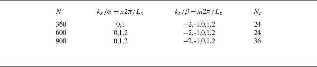
Cavalieri & Nogueira (Reference Cavalieri and Nogueira2022) considered 24 controllability modes for each combination of wavenumber pair, making a total of
 $N=600$
modes. This basis was found to be large enough for a reasonably accurate representation of first- and second-order turbulence statistics at a Reynolds number of
 $Re=1200$
. In the present study, we consider flows with Reynolds numbers up to
 $Re=3000$
, and larger bases were necessary in order to keep the same degree of accuracy of the ROM. We considered 36 controllability modes for each wavenumber pair, leading to a total of
 $N=900$
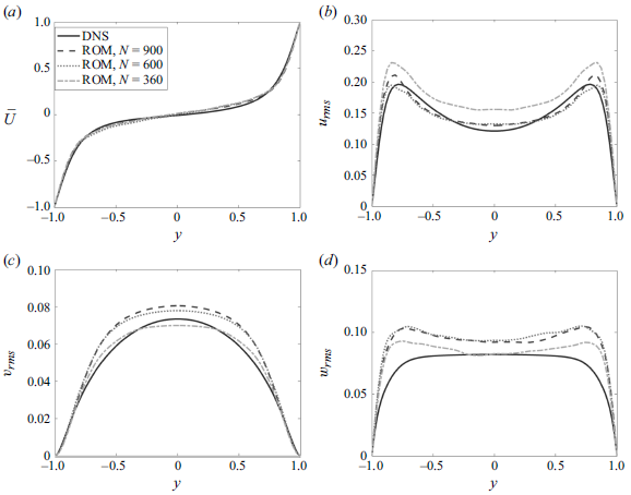
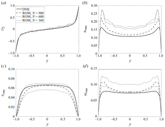
modes in the basis. As shown in Appendix A, this number of modes was found to be sufficient to produce smooth mean and root-mean-square (r.m.s.) velocity profiles which are in reasonable agreement with DNS data, whose details are given in § 4. The number of points used to discretise the domain in the streamwise and spanwise directions is defined so as to satisfy the Nyquist criterion for dealiasing, given the number of wavenumbers kept in the basis. We therefore set
 $N_x=10$
,
 $N_z = 14$
. The wall-normal direction is discretised with
 $N_y=65$
points.
Inserting the modal expansion (2.2) into the governing equations (2.1) and taking the inner product with
 $\phi _i$
leads to the following system of equations:
 \begin{equation} \frac {\text{d}a_i}{\text{d}t} = \frac {1}{\textit{Re}}\sum _j L_{ij}a_j + \sum _j\tilde {L}_{ij}a_j + \sum _j\sum _k Q_{ijk}a_ja_k, \end{equation}
where
 \begin{equation} L_{ij} = \langle \nabla ^2\phi _j,\phi _i \rangle, \end{equation}
 \begin{equation} \tilde {L}_{ij} =- \left \langle [(\phi _j \cdot \nabla){\textbf{u}}_0 + ({\textbf{u}}_0 \cdot \nabla)\phi _j], \phi _i\right \rangle, \end{equation}
 \begin{equation} Q_{ijk} = -\left \langle (\phi _j \cdot \nabla)\phi _k,\phi _i \right \rangle, \end{equation}
and the inner product,
 $\langle \cdot \rangle$
, is defined as
 \begin{equation} \left \langle \textbf{f}, \textbf{g} \right \rangle = \frac {1}{2 L_x L_z}\int _{0}^{L_z}\int _{-1}^{1}\int _{0}^{L_x} \textbf{f}(x,y,z)\textbf{g}(x,y,z)\text{d}x\text{d}y\text{d}z. \end{equation}
The time history of mode coefficients is obtained by initiating the system of (2.4) with a random condition and then performing integration using a standard 4th/5th Runge–Kutta scheme.
2.1. Reduced-order model with extra forcing term
We now consider the Navier–Stokes system subject to a steady body force,
 $\mathbf{F}$
, constant in
 $x$
and
 $z$
but varying in
 $y$
, to which we apply a similar modal decomposition
 \begin{equation} \mathbf{F} = \sum _{j=1}^{N_s} b_j\phi _{0_j}(y), \end{equation}
wherein the spatial structure of the forcing is given by a linear combination of Stokes modes,
 $\phi _{0_j}$
, corresponding to
 $k_x=k_z=0$
, weighted by their coefficients,
 $b_j$
. These are the same modes used to describe the mean flow in the ROM basis, but with different coefficients. As each wavenumber pair in the ROM basis has 36 associated controllability modes, in principle 36 Stokes modes are available in the forcing space. However, we consider a forcing term that is aligned with the streamwise direction; therefore, Stokes modes that possess non-zero spanwise velocity components are discarded. Furthermore, due to the geometry of the flow, we restrict the forcing basis to be composed only of modes that are anti-symmetric with respect to the origin. With these restrictions, the forcing basis is reduced to
 $N_s=9$
Stokes modes. Figure 2 shows the structure of the first four Stokes modes used in the simulations that will be described in what follows.
Wall-normal structure of first four Stokes modes that compose the forcing term.

Applying the Galerkin projection described above yields a new forced system
 \begin{equation} \frac {\text{d}a_i}{\text{d}t} = \frac {1}{\textit{Re}}\sum _j L_{ij}a_j + \sum _j\tilde {L}_{ij}a_j + \sum _j\sum _k Q_{ijk}a_ja_k + \sum _j^{N_s}F_{ij}b_j, \end{equation}
where
 \begin{equation} F_{ij} = \left \langle \phi _{0_j},\phi _i \right \rangle. \end{equation}
Our goal in this study is to devise a control strategy using the forcing term. This is achieved by seeking a linear combination, or a set of
 $b_j$
coefficients, that reduces a functional which represents the total fluctuation energy, given by
 \begin{equation} E = \frac {1}{2} \langle {\mathbf{u}}^{\prime}, {\mathbf{u}}^{\prime} \rangle = \frac {1}{2}\big\langle \big( {\mathbf{u}} - \overline {\mathbf{U}} \big),\big( {\mathbf{u}} - \overline {\mathbf{U}} \big) \big\rangle, \end{equation}
where
 ${\mathbf{u}}^{\prime}$
are fluctuations around the turbulent mean flow,
 $\overline {\mathbf{U}}$
(and which should not be confused with velocity fluctuations around the laminar Couette solution,
 $\mathbf{u}$
). Using the modal expansion defined in (2.2) and the orthonormality property of the basis leads to
 \begin{equation} E = \frac {1}{2} \left [ \sum _{i} a_i^2 - \sum _{i} a_{0_i}^2 \right], \end{equation}
where
 $a_{0_i}$
are the modal coefficients of the mean-flow modes (modes with zero streamwise and spanwise wavenumbers). The optimisation is carried out considering a time horizon divided into two segments: the first one,
 $0 \leqslant t \lt t_1$
, in which the forcing term is activated, and a second one,
 $t_1 \leqslant t \leqslant t_2$
, in which the forcing is turned off. The forcing is turned on and off following smooth ramps of the form
 $ \mathbf{F}(0.5+0.5\tanh (0.01t))$
,
 $-\mathbf{F}(0.5+0.5$
 $\tanh (0.01(t-t_{1})))$
. The functional then takes the form
 \begin{equation} \mathcal{J} = \frac {2}{t_2}\underbrace {\left [\int _{0}^{t_1} E(t) \text{d}{t}\right.}_{\text{forcing on}} + \underbrace {\left. \int _{t_1}^{t_2} E(t) \text{d}{t}\right]}_{\text{forcing off}}, \end{equation}
where
 $t_2$
is the total time horizon for the computation of the functional. With this approach, we seek a forcing term that reduces turbulent fluctuations upon acting only over a limited time period and that keeps the fluctuations to a minimum after it is disabled. The optimisation of the forcing coefficients,
 $b_j$
, is performed iteratively using a gradient-descent algorithm
 \begin{equation} b_j^{n+1} = b_{j}^n - \epsilon \frac {\partial \mathcal{J}^n}{\partial b_j^n}, \end{equation}
where the superscript
 $n$
denotes the iteration number, and
 $\epsilon$
is a learning rate. The Jacobian is approximated through a first-order finite-difference scheme
 \begin{equation} \frac {\partial \mathcal{J}}{\partial b_j^n} \approx \frac {\mathcal{J}^n \big(b_j^n+\delta b_j\big)-\mathcal{J}^n\big(b_j^n\big)}{\delta b_j}. \end{equation}
Values between
 $\delta b_j = 10^{-2}{-}10^{-4}$
and
 $\epsilon = 10^{-3}{-}10^{-4}$
were used, depending on the Reynolds number, in order to obtain a smoothly converging algorithm. We anticipate that the optimisation procedure will lead to laminarisation of the flow for all Reynolds numbers considered in this work,
 $Re = 1000,2000,3000$
. The number of iterations required to achieve laminarisation increased with Reynolds number, varying typically between
 ${\backsim}7$
, for
 $Re= 1000$
to
 ${\backsim}20$
for
 $Re = 3000$
. At each iteration, the nine-DoF Jacobian is computed through (2.16). Therefore, the optimisation procedure requires, for the highest Reynolds numbers tested here, approximately two hundred simulations. Besides the simplifying aspect of solving a system of ordinary differential equations instead of a system of partial differential equations, the computational gain of using a ROM-based approach to perform this task is considerable. For instance, the DNS at
 $Re=3000$
performed in the present study (with
 $\mathcal{O}(10^7)$
DoF) requires
 ${\sim} 10^4$
core hours using 2.60 GHz Intel Xeon CPU E5-2640 cores. The corresponding ROM simulation at the same
 $Re$
(
 $\mathcal{O}(10^3)$
DoF), on the other hand, is of the order of a few minutes.
The kind of forcing optimisation proposed here is therefore much more affordable with the ROMs. A less expensive (albeit more difficult to formulate) way of computing the gradient is using adjoint methods. However, since the number of DoFs of the forcing term is small, the procedure described here provides a more straightforward and affordable method to assess the suitability of the ROMs to derive control methods. Furthermore, it is worth emphasising that our goal is to conduct an exploratory study to assess the possibility of designing a control method using the ROM framework. Therefore, in this first step we are not concerned with the feasibility of applying the optimal forcing in experiments. This involves imposing further spatial restrictions to the forcing, or considering forcing by wall motion or blowing and suction; however, this is something that we leave to future studies. Here, we prefer to avoid such restrictions and focus on the physical mechanisms of the derived control method.
In the following, the results of the controlled ROMs are discussed and we explore in detail the mechanisms that lead to turbulence disruption. The reader is referred to Cavalieri & Nogueira (Reference Cavalieri and Nogueira2022) for more details about the numerical methods used to obtain the modal basis and to integrate (2.4) and (2.10) in time.
3. Results: controlled ROM
We first present a detailed analysis of controlled and uncontrolled systems at
 $Re=1000$
. The effects of control at higher Reynolds numbers are then discussed in section § 3.2. In total, the systems were integrated in time for 2500 time units, with the forcing being turned off at
 $t_1=1500$
. Figure 3(a) shows the evolution of the control functional in the iterative process of finding the optimal forcing. Laminarisation is reached at the fifth iteration, and the corresponding forcing structure is shown in figure 3(b). It has an anti-symmetric shape, with two large peaks of equal amplitude and opposite signs in the near-wall region,
 $y \pm 0.8$
, and two smaller peaks near the centre of the channel. This forcing was subsequently used to run longer simulations, integrated up to 4000 time units, in which an initial time segment without the forcing (standard Couette flow) was included. Analysis of the control effect can then be carried out by comparing flow statistics in each time segment.
Optimisation of the forcing term at
 $Re= 1000$
: (a) evolution of the functional with increasing number of iterations; (b) forcing structure, computed from (2.9), at the end of the iterative process.

Figure 4 shows a time history of the modal coefficients during the simulation along with mean and r.m.s. velocity profiles computed at each time segment separately. The statistics are computed considering the second half of each time segment. After activation of the control, fluctuations of the modal coefficients cease rapidly and all of them fall to zero, except those constituting the mean flow,
 $k_x=k_z=0$
. These modes, also known as Stokes modes, are the same ones used in the definition of the forcing (2.9). They are steadily excited by the forcing and assume constant values. This indicates that the time-averaged forced flow profile shown in figure 4(b) actually corresponds to a steady-state solution of the forced flow or, in other words, a new laminar state. In this new laminar state, the velocity reaches zero at a position much closer to the walls (approximately
 $y \pm 0.45$
, as opposed to the centre of the channel in uncontrolled Couette flow), with small positive and negative oscillations around the centre. When the control is turned off again (time segment III), all modal coefficients fall to zero and the flow returns to the laminar Couette state. Figure 4(c) presents r.m.s. profiles of velocity fluctuations. As can be inferred from the discussion above, in time segments II and III all fluctuations are zero, following the laminarisation of the flow.
Results of controlled ROM simulations at
 $Re=1000$
, where forcing is turned on and off. (a) Time evolution of the model coefficients,
 $a_i$
. The vertical dashed lines indicate time instants when the control is turned on and off; (b) time-averaged flow profiles corresponding to time segments I (——), II (– – –) and III (
 $\cdots\cdots$
). (c) r.m.s. velocity profiles of
 $u$
(blue),
 $v$
(yellow) and
 $w$
(red). Line style is the same as in (b).

Figure 5 further illustrates the control effect on the velocity fields. Typical streamwise velocity snapshots taken in the three time zones are displayed. Consistent with the trends discussed above, the snapshot taken in the controlled time zone reveals a drastic reduction of the sheared region, whereas that of time zone III shows the canonical laminar Couette profile.
Snapshots of streamwise velocity in the
 $y{-}z$
plane taken at time instants within segments I, II and III, highlighted in figure 4: (a)
 $t=500$
; (b)
 $t=2500$
; (c)
 $t=3500$
. The Reynolds number is
 $Re=1000$
.

3.1. Control mechanism
We now discuss the physical mechanisms by which turbulence is disrupted. We start by analysing the energy budget, which is obtained by multiplying the governing equation, (2.10), by
 $a_i$
 \begin{equation} \frac {\text{d}(a_i^2/2)}{\text{d}t} = \underbrace {\frac {1}{\textit{Re}}\sum _j L_{ij}a_i a_j}_{\text{$D_i$}} + \underbrace {\sum _j\tilde {L}_{ij}a_i a_j}_{\text{$I_{i_1}$}} + \underbrace {\sum _j \sum _k Q_{ijk}a_i a_j a_k}_{\text{Nonlinear Int.}} + \underbrace {\sum _j^{N_s}F_{ij}a_ib_j}_{\text{$I_{i_2}$}}. \end{equation}
In plane Couette flow with zero pressure gradient, the fluid is driven by the motion of the walls, and the energy input to the system comes from the shear created by the velocity profile. This is represented by the second term on the right-hand side of (3.1), named
 $I_{i_1}$
. The forcing term provides an extra energy input to the controlled ROMs, which is denoted as
 $I_{i_2}$
. Energy is dissipated through the viscous term,
 $D_i$
. The total inputs,
 $I_1$
and
 $I_2$
and dissipation,
 $D$
, can be computed from the sum of their respective modal contributions,
 $I_1 = \sum _{i}^N I_{i1}$
,
 $I_2 = \sum _{i}^N I_{i2}$
,
 $D = \sum _{i}^N D_{i}$
. The nonlinear interaction term, on the other hand, is conservative. Its role is to distribute energy among different wavenumbers, but, for an incompressible flow, it has zero net contribution to the energy budget,
 $\sum _{i,j,k}Q_{i,j,k}=0$
(Schmid & Henningson Reference Schmid and Henningson2012).
Figure 6 summarises the behaviour of the kinetic energy in uncontrolled and controlled ROMS. Panels (a) and (b) show flow trajectories in the subspace defined by the total
 $I_1$
input and the total dissipation
 $D$
, in uncontrolled and controlled systems, respectively. In a turbulent state, the trajectory oscillates around the diagonal, alternating periods of increasing (below the diagonal) and decreasing (above the diagonal) kinetic energy (Kawahara & Kida Reference Kawahara and Kida2001). This is precisely the case for the uncontrolled system. In the controlled ROM, the trajectory oscillates for some time around the diagonal; but when the forcing is turned on, it eventually escapes the near-diagonal region, approaches the
 $D$
axis and falls to the laminar Couette value when the forcing is turned off again. This is also illustrated in panel (c), which presents the evolution of inputs and dissipation following the time windows of active and inactive control. In the first part of the simulation, before the forcing term is turned on,
 $I_1$
and
 $D$
are balanced (in a statistical sense), and the total kinetic energy oscillates. When the control is turned on (
 $t\gt 1500$
), the main energy input,
 $I_1$
, falls sharply to the laminar Couette value. After a short transient, the flow reaches a new laminar state where the energy input from the forcing term
 $I_2$
and the dissipation remain constant (and in perfect balance) at a non-zero value. After the control is turned off again, the flow returns to the laminar Couette state.
Energy budget analysis for ROMs at
 $Re=1000$
. Panels (a) and (b) show phase portraits in the input–dissipation subspace for uncontrolled and controlled ROM simulations, respectively. Input and dissipation are in balance on the dashed diagonal line. The blue and green dots in (b) indicate the laminar states for the controlled and uncontrolled flows, respectively. (c) Presents the time evolution of total inputs and dissipation terms as the forcing is turned on and off. Inputs and dissipation are normalised by the laminar values for Couette flow.

This analysis reveals that the control acts globally by annihilating the main energy input,
 $I_1$
. This is achieved by a strong reduction of the shear on the central part of the channel, as evidenced by the instantaneous velocity contours shown in figure 5. Alternatively, further insight into the control mechanism can be gained by a ‘modal’ characterisation of its effect. This can be done, for instance, by inspection of the modes responsible for the average energy production. Averaging (3.1) for long simulation times leads to
 \begin{equation} 0 = \underbrace {\frac {1}{\textit{Re}}\sum _j L_{ij}\overline {a_i a_j}}_{\overline {D}_i} + \underbrace {\sum _j \tilde {L}_{ij}\overline {a_ja_j}}_{\overline {I}_{i_1}}+ \underbrace {\sum _j \sum _k Q_{ijk}\overline {a_i a_j a_k}}_{\text{Nonl. Int.}} + \underbrace {\sum _j^{N_s}F_{ij}b_j \overline {a_i}}_{\overline {I}_{i_2}}, \end{equation}
where the overbar denotes time averaging. Figure 7 shows modal distributions of energy inputs in the uncontrolled (
 $\overline {I}_{i_1}$
) and controlled (
 $\overline {I}_{i_2}$
) ROMs, ranked in descending order. These are computed by performing the time averages of (3.2) in time segments I and II of the simulations, respectively. In the uncontrolled ROM, energy production is distributed over a large number of modes. The shapes of the two modes associated with the largest energy production, circled in panel (a), are shown in (b) and (c). They display patterns of low and high streamwise velocity interspersed with streamwise vortices which characterise the classic streak-roll mechanism. Their associated wavenumbers are (
 $k_x/\alpha, k_z/\beta) = (0,1)$
, and they correspond to the largest streaks/rolls in the basis. Subsequent modes in the energy-ranking order (not shown here for conciseness) correspond to oblique waves (
 $k_x/\alpha \neq 0$
) and smaller streaks (
 $k_x/\alpha =0, |k_z/\beta | = 2$
). In the controlled ROM, on the other hand, all the input is provided via mean-flow modes,
 $(k_x/\alpha, k_z/\beta)=(0,0)$
, with only two modes receiving practically the entirety of the energy.
Modal distribution of energy input in uncontrolled and controlled ROMs. Panels (a) and (d) show averaged modal energy inputs,
 $\overline {I}_{i_1}$
and
 $\overline {I}_{i_2}$
, ranked in descending order. Modes associated with the circled inputs in (a) and (d) are displayed in (b)–(c) and (e)–(f) in the uncontrolled and controlled ROMs, respectively. Contours correspond to the streamwise velocity component,
 $u$
, and the arrows represent the wall-normal,
 $v$
, and spanwise,
 $w$
, components.

The largest streaks and rolls described in the basis (
 $(k_x/\alpha, k_z/\beta) = (0,1)$
) are, therefore, the flow structures most affected by the forcing. This suggests that the forcing disrupts the self-sustaining processes. This mechanism, which consists in the linear amplification of streaks by streamwise vortices, followed by their ‘bursting’ via a secondary instability that leads to the regeneration of new streamwise vortices, is at the core of self-sustaining processes in wall-bounded turbulence at different scales (Hamilton et al. Reference Hamilton, Kim and Waleffe1995; Waleffe Reference Waleffe1997; Jiménez & Pinelli Reference Jiménez and Pinelli1999; Hwang & Cossu Reference Hwang and Cossu2010b
; Flores & Jiménez Reference Flores and Jiménez2010; Hwang Reference Hwang2015; Hwang & Bengana Reference Hwang and Bengana2016; de Giovanetti, Sung & Hwang Reference de Giovanetti, Sung and Hwang2017). By blocking the linear energy transfer to streaky structures from the sheared base flow, the control mechanism disrupts one the stages of the self-sustaining process: the linear amplification of streaks via the lift-up mechanism. This will be further corroborated by the results of the transient growth analysis shown in the following.
Further insight into the control mechanism can be gained by exploring the linear stability characteristics of the forced flow, which we address now. This analysis (and all linear analyses performed throughout this study) considers laminar flow solutions, in both forced and unforced systems, as base flows. The forced laminar state can be computed from the steady-state solution of (2.10)
 \begin{equation} \left ( \frac {1}{\textit{Re}}\sum _jL_{ij} + \sum _j \tilde {L}_{ij} \right)a_j^{lam} = -\sum _j^{N_s} F_{ij}b_j. \end{equation}
We then consider the evolution of perturbations around the new laminar solution,
 $a_j = a_j^{lam}+ a_j^{\prime}$
. Substituting this expression in (2.10) and linearising about the new laminar solution yields
 \begin{equation} \frac {\text{d} a_j^{\prime}}{\text{d}t} = \sum _j \hat {L}_{ij}a_j^{\prime}, \end{equation}
where
 \begin{equation} \hat {L}_{ij} = \frac {1}{\textit{Re}}L_{ij} + \tilde {L}_{ij} + \sum _k Q_{ijk} a_k^{lam} + \sum _k Q_{ikj}a_k^{lam}, \end{equation}
is the new linear operator. Modal instability mechanisms can be assessed through the eigendecomposition of the linear operator
 \begin{equation} \hat {L}_{ij} =\mathcal{Q}\Psi \mathcal{Q}^{-1}, \end{equation}
where the columns of matrix
 $\mathcal{Q}$
are the eigenvectors and the diagonal matrix
 $\Psi$
contains the associated eigenvalues,
 $\psi = \psi _r + i\psi _i$
. The system is linearly unstable if there is at least one mode with
 $\psi _r\gt 0$
, and this can provide a possible path to transition over long time periods. Over short time periods, however, transition to turbulence can be achieved (or turbulence can be maintained), even in the absence of modal instabilities, by transient growth of disturbances due to the non-normality of the linear operator (Schmid & Henningson Reference Schmid and Henningson2012). The importance of transient growth for transition (Henningson & Reddy Reference Henningson and Reddy1994) and for the dynamics of near-wall turbulence (Schoppa & Hussain Reference Schoppa and Hussain2002) is now well established. Moreover, a recent study by Lozano-Durán et al. (Reference Lozano-Durán, Constantinou, Nikolaidis and Karp1971) has conclusively shown that transient growth is dominant over other linear amplification mechanisms regarding their role in sustaining near-wall turbulence. They have shown that transient growth alone is capable of sustaining wall turbulence through a series of numerical experiments where other kinds of instabilities (exponential instabilities, neutral modes, parametric instabilities) are artificially suppressed. Modal instabilities, on the other hand, even when present, only account for a small fraction of the turbulent kinetic energy. It is therefore important to characterise the potential of the new laminar solution in amplifying disturbances through non-modal mechanisms. Considering the solution of the initial-value problem (3.4)
 \begin{equation} a_j^{\prime}(t) = \text{e}^{\hat {L} t}a_{j_0}^{\prime}, \end{equation}
with
 $a_{j_0}^{\prime}$
an initial perturbation, the maximum amplification reached at a given time instant,
 $G(t)$
, is given by
 \begin{equation} G(t) = \max _{a_{j_0}^{\prime} \neq 0} \frac {||a^{\prime}_j (t)||^2}{||a^{\prime}_{j_0}||^2} = ||\text{e}^{\hat {L} t}||^2, \end{equation}
where
 $||\cdot ||$
denotes an Euclidean norm and
 $G(t)$
is given by the largest singular value,
 $\sigma _1^2$
, of
 $\text{e}^{\hat {L} t}$
. Figure 8 compares modal and non-modal linear stability characteristics of the new laminar solution achieved with the controlled ROM, compared with laminar Couette flow. Notice that the forced flow profile, computed from the linear ROM (3.3) and displayed in (a), is identical to time-averaged velocity profiles shown in figure 4, computed from the nonlinear simulation. This further demonstrates that the forcing leads the flow to a new laminar state at this
 $Re$
. The eigenvalue spectra, computed from equation, (3.6) are shown in panel (b). The eigenvalues were computed with the MATLAB function eig, which uses a generalised Schur decomposition algorithm. The accuracy of the computation can be estimated by the residual norm of the error,
 $| \hat {L}_{ij}\mathcal{Q} - \mathcal{Q}\Psi |/ |\hat {L}_{ij}|$
, which was equal to
 $2 \times 10^{-14}$
. Both laminar states are linearly stable (all
 $\psi _r\lt 0$
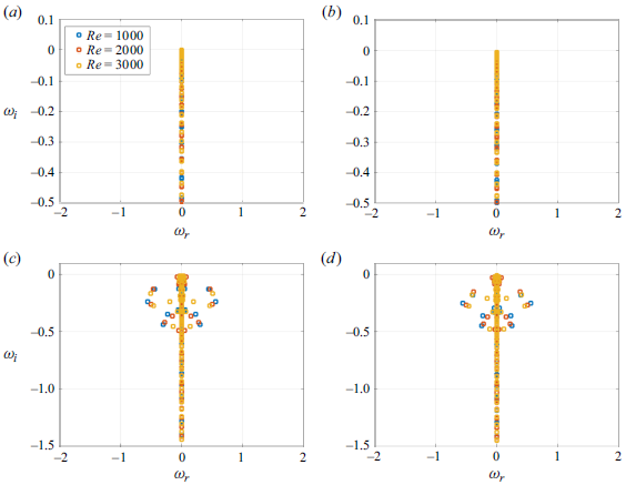
). The least stable eigenvalues of the two solutions are almost identical, which suggests that the two base flows possess similar modal stability behaviour. Their transient growth behaviour, on the other hand, is strikingly different. The maximum transient amplification supported by the new base flow is reduced by a factor of sixteen with respect to that of Couette flow. This directly affects the ability of the new laminar base flow in supporting non-modal instabilities via the lift-up mechanism, which hinders the ability of the flow in sustaining a turbulent state. This is consistent with the return to the laminar Couette state after the control is disabled. Apart from the large peaks in the transient growth curves, smaller peaks can also be seen at much earlier times,
 $t \approx 15$
. The presence of double peaks is due to the fact that the linear operator of the ROM,
 $\hat {L}_{ij}$
, describes modes with different wavenumbers. Each peak is therefore associated with a flow structure at a given wavenumber. In Appendix B, transient growth is computed with the Orr–Sommerfeld–Squire system, which allows a separate analysis for each wavenumber pair,
 $(k_x, k_z)$
. The main peak of
 $G(t) \approx 1100$
in figure 8(c) is associated with the amplification of the largest streaks in the basis,
 $(k_x/\alpha, k_z/\beta)=(0,1)$
, which can be seen by comparing figures 8(c) and 26(a). The small peak, on the other hand, is a signature of oblique waves,
 $(k_x/\alpha, k_z/\beta)=(1,2)$
. Notice how it is quite similar to the curve shown in figure 26(c) for
 $Re=1000$
.
Linear stability characteristics of the new laminar solution obtained with the controlled ROM, compared with canonical Couettte at
 $Re=1000$
. (a) New laminar velocity profile; (b) eigenvalue spectrum of the linear operator; (c) transient growth analysis.

3.2. Higher Reynolds numbers
Comparison of control results at
 $Re=1000, 2000, 3000$
. (a) Wall-normal structure of the forcing term. Panels (b), (c) and (d) show comparisons between the new laminar base flows (dashed lines) and the turbulent mean flows (solid lines) without the forcing.

We now discuss control results obtained at higher Reynold numbers. The optimisation procedure described previously was applied to flows at
 $Re=2000$
and 3000. The steady forcing was found to lead the flow to a new laminar state in both cases, as observed for
 $Re=1000$
. The shape of the optimal forcing term and the new laminar base flows are displayed in figure 9. The forcing shape at intermediate iterations was found to evolve smoothly until convergence is achieved; this is not shown here for compactness. As the Reynolds number is increased, the peaks observed in the forcing structure near the wall become sharper and increase in amplitude, shifting progressively towards the wall. These trends follow the changes in the mean velocity gradient for turbulent Couette flow, which also becomes larger and sharper in the vicinity of the wall with increasing Reynolds number. At
 $Re=2000$
and 3000 larger positive and negative oscillations of the forcing term are observed at the central part of the channel. Such oscillations are likely related to the low dimensionality of the basis, particularly with the number of controllability modes taken at each wavenumber pair. At higher Reynolds number, the low number of controllability modes in the basis makes it difficult to represent a forcing term with sharp gradients, leading to the observed wavy behaviour, which would probably become more pronounced with increasing Reynolds number. This issue could be mitigated with the addition of more controllability modes with increasing Reynolds numbers, leading to larger ROMs. However, it will later be seen that despite the oscillatory nature of the obtained body forces, these are able to relaminarise the flow in DNS. Therefore, we prefer to keep the same ROM for all Reynolds numbers tested.
It should be pointed out that the wavy structure of the forcing at
 $Re=2000$
and
 $3000$
would be quite difficult to reproduce experimentally. However, as pointed out above, this study should be seen as a first step in the use of the ROM framework to design turbulence control methods. Therefore, here, we choose to focus our attention on the physical mechanisms underpinning the suppression of turbulence, rather than on the feasibility of the method in an experimental application. Designing more realistic (near-wall) body forces is something we will address in future studies.
The new laminar profiles of the forced flows are shown in figure 9(b)–(d). These profiles, computed as steady-state solution of the linearised ROM, equation (3.3), were found to be identical to velocity profiles computed directly from the nonlinear simulation, equation (2.10), during the application of the forcing. They correspond, therefore, to steady-state solutions to the forced flow equations. These solutions at the three Reynolds numbers share some similar features. Although they are characterised by slightly lower wall shear stresses with respect to the turbulent mean flows, their associated velocity gradients eventually become larger further from the wall, increasing the rate of velocity decay. The laminar profiles reach zero velocity at a wall-normal position much closer to the wall, and then oscillate around zero over an extended central region. This confines the shear to near-wall regions, as can be inferred from the instantaneous velocity field depicted in figure 5(b) for
 $Re=1000$
.
Figure 10 shows the temporal evolution of inputs and dissipation in the
 $Re=2000, 3000$
simulations. As observed previously for
 $Re=1000$
, the main energy input from the sheared flow,
 $I_1$
, is completely disrupted upon activation of the forcing term. Also as observed in the lower-Reynolds-number case, the flow relaminarises when the forcing is switched off. All of these trends indicate that the control mechanism is the same in the three Reynolds numbers explored.
Energy budget analysis for ROMs at
 $Re=2000$
(a) and
 $Re=3000$
(b). Inputs and dissipation are normalised by the laminar values for Couette flow.

The linear stability characteristics of the controlled ROMs at
 $Re=2000, 3000$
were explored, following the analysis laid out in § 3.1. At all Reynolds numbers, the new laminar state achieved with the forcing is found to be linearly stable. The transient growth of disturbances was found to be massively reduced with respect to the laminar Couette flow, in line with the observations made for
 $Re=1000$
. This is illustrated in figure 11. For the laminar Couette base flow, the non-modal amplification increases with
 $Re$
, as expected. For the base flow of the controlled ROMs, however, the maximum transient amplification varies very little for the three Reynolds numbers, remaining close to
 $G_{max} \sim 100$
. The difference in transient amplification between controlled and uncontrolled ROMs therefore increases with increasing Reynolds number, reaching a reduction factor of a hundred for
 $Re=3000$
. The non-monotonic decay of
 $G(t)$
for the forced base flow is again due to the fact that the linear operator of the ROM describes modes with different wavenumbers. The double peaks in the transient curves are likely associated with the signature of flow structures with different wavenumbers.
In the control study of Kühnen et al. (Reference Kühnen, Scarselli, Schaner and Hof2018a
) on pipe flows, it was found that relaminarisation occurred whenever the maximum transient growth of the controlled mean-flow profile was reduced below a given threshold, which was found to be
 $G_{max}^{t} \approx 65$
. This laminarisation threshold was found to hold for different control approaches, in both experiments and simulations. The results shown here suggest that a similar threshold exists for Couette flow, although in the present case it seems to be higher, probably slightly above
 $G_{max}^{t} \approx 100$
. As discussed above, the transitional Reynolds number for plane Couette flow identified experimentally is around
 $Re_t \approx 325$
(Bottin et al. Reference Bottin, Dauchot and Daviaud1997, Reference Bottin, Dauchot, Daviaud and Manneville1998). One can argue that this transitional Reynolds number sets the threshold
 $G_{max}^{t}$
necessary for turbulence to sustain itself. In this sense, we can interpret the effect of the optimal forcing as that of reducing the ‘effective’ Reynolds number of the controlled flow below
 $Re_t$
. This, in turn, reduces the maximum transient growth below
 $G_{max}^t$
. This is corroborated by the results of figure 11(b), which show that the values of
 $G_{max}$
for the controlled ROMs are quite close to that obtained from the laminar Couette base flow at
 $Re=300$
. Results of nonlinear simulations performed at
 $Re=300$
further confirmed that a turbulent state cannot be sustained in the ROM at this Reynolds number, complete laminarisation occurring approximately 100 time units after the start of the simulations.
Transient growth behaviour of ROMs at different Reynolds numbers. (a) Comparison between laminar Couette flow and the new laminar (controlled) state at
 $Re=1000, 2000, 3000$
; (b) zoomed view of the transient growth curves for controlled ROMs. Their maximum transient amplification is found to be almost constant, and close to that obtained with a laminar Couette profile at
 $Re=300$
.

As mentioned above, the stability characteristics of forced and non-forced systems can also be investigated using the full Orr–Sommerfeld–Squire equations, considering the linearisation of the full Navier–Stokes system, without model reduction, which is described in Appendix B. The advantage of working with the Orr–Sommerfeld–Squire system is that the analysis can be carried out separately for a given wavenumber pair,
 $(k_x, k_z)$
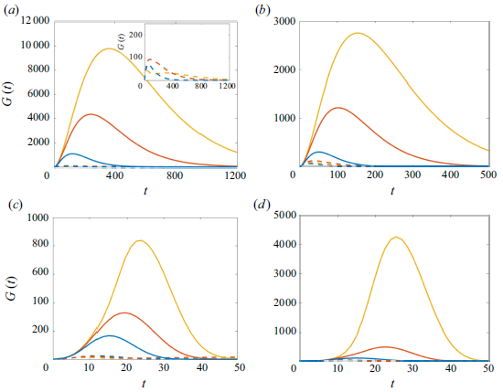
, as opposed to the analysis performed through (3.8), which does not allow that separation. Moreover, the results show trends for the two laminar states without truncation of the system to a reduced number of modes, allowing a confirmation of the trends obtained with the ROM. Figures 24–26 show modal and non-modal stability characteristics of the forced base flows for combinations of wavenumbers
 $k_x/\alpha = 0, 1$
and
 $k_z/\beta = 1, 2$
. The forced flow is found to be linearly stable for all wavenumbers at
 $Re=1000$
. At
 $Re=2000,3000$
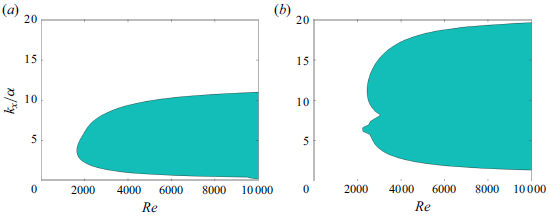
the forced laminar states are stable for the wavenumber combinations contained in the ROM, but unstable at higher streamwise wavenumbers. As will be discussed shortly in section § 4, in the DNS this instability leads the flow to a state of weak turbulence, in which velocity fluctuations and transient growth are massively reduced. The largest transient amplification is obtained with
 $(k_x/\alpha, k_z/\beta)=(0,1)$
, which correspond to the largest streak/roll structures contained in the ROM basis. We note that the transient growth curves for this wavenumber pair, displayed in figure 26(a), are very close to those described by (3.8) (and displayed in figure 11
a) for both the forced and unforced cases, showing that the non-modal behaviour of the flow is mainly underpinned by these structures. Smaller streaks,
 $(k_x/\alpha, k_z/\beta) = (0,2)$
and structures with
 $k_x \gt 0$
, corresponding to oblique streaks/rolls, have lower transient amplifications. Nonetheless, for all wavenumber combinations tested, the maximum non-modal growth is massively reduced in the forced laminar state.
It is also important to quantify the net energy saving that would be possible with this kind of control if it could be reproduced experimentally. This can be estimated from the results of the energy budget analyses above. The terms
 $I_1$
and
 $I_2$
represent the two sources of energy to the flow: the shear motion of the walls and the body force. The term
 $I_1$
is present in both the controlled and uncontrolled flows, whereas
 $I_2$
only assumes non-zero values when the control is active. Using a rationale similar to that of Kühnen et al. (Reference Kühnen, Song, Scarselli, Budanur, Burak, Riedl, Willis, Avila and Hof2018b
), the net energy saving can be expressed as
 \begin{equation} S = \frac {\overline {I}_{1}^{T}-\big(I_{2}+I_{1}^{C}\big)}{\overline {I}_{1}^{T}}, \end{equation}
where
 $\overline {I}_{1}^{T}$
is the reference shear input, computed as the time average of
 $I_1$
in the first segment of the simulation (with the control off). Here,
 $I_{1}^{C}$
is the shear input in the controlled part of the simulations. Figure 12 shows the time series of energy savings from the instant when the forcing is turned on (
 $t=1500$
) up to the end of the simulation.
Net energy savings as a function of time for
 $Re=1000$
(a),
 $Re=2000$
(b) and
 $Re=3000$
(c). The dashed line marks the theoretical limit for energy savings, which occurs when the forcing is disabled and the flow returns to the laminar Couette state.

As the forcing is turned on, the energy expenditure decreases and then remains constant after the flow reaches the new laminar state. The net energy savings achieved with the control on are
 $S = 48.6\,\%, 44.97\,\%, 45.34\,\%$
for the three Reynolds numbers tested. The flow goes back to the laminar Couette state upon removal of the forcing, and it will tend to remain in this state indefinitely in the simulation, as the laminar Couette base flow is linearly stable. (Of course in an experiment finite-amplitude perturbations are likely to be generated by the experimental apparatus, which would lead the flow to a turbulent state again via transient growth. Therefore, if this type of control were used in an experiment, it would probably have to operate intermittently.) In this condition,
 $I_{1}^{C}=1$
(normalising by laminar Couette values) and
 $I_2=0$
, and the energy saving then reaches a theoretical limit, which represents the difference in the energy expenditure necessary to maintain laminar turbulent flows at a given Reynolds number. This limit is equal to
 $S = 77.3\,\%, 86\,\%, 89.6\,\%$
for
 $Re=1000,2000,3000$
.
3.3. Control robustness
In order to assess the robustness of the control mechanism, two sets of additional tests were performed. In the first set, simulations are initiated by the laminar solution plus random perturbations,
 $a_{j}(t=0) = a_j^{lam} + A \tilde {a}_j^{\prime}$
, with perturbations
 $\tilde {a}_j^{\prime}$
generated numerically and following a uniform distribution. The goal of this first set of tests was to vary the perturbation amplitude,
 $A$
, and assess whether there is a limit amplitude beyond which the control becomes ineffective. The amplitudes were varied over a broad range,
 $A = 10^{-1}$
–
 $10^3$
, and the forcing was turned on at the beginning of the simulations. In all cases the flow returned to the controlled laminar state after a quick transient. This suggests an expansion of the basin of attraction of the laminar solution in the forced flow. This will be briefly discussed in section § 5. Figure 13 shows time histories of modal coefficients in simulations started with initial conditions of increasing amplitudes.
Robustness tests for controlled ROMS at
 $Re=3000$
to random initial conditions of different amplitudes. Panels show (a)
 $A=1$
; (b)
 $A=10^1$
; (c)
 $A=10^2$
. The inset in (c) displays zoomed views. The forcing term is turned on in the beginning of the simulations.

In the second set of tests, the robustness of the control mechanism to off-design Reynolds numbers was assessed by using the forcing term obtained through the optimisation algorithm at
 $Re = 2000$
in simulations carried out at progressively higher Reynolds numbers. Some results are shown in figure 14. At small departures from the design condition, for instance at
 $Re=2100$
, the control still produces order-of-magnitude reductions of velocity fluctuations, and after the control is disabled the flow stays in the laminar Couette state. However, at this
 $Re$
we also observe an increase in velocity fluctuations at the controlled segment of the simulations with respect to the baseline case,
 $Re = 2000$
. Particularly, the increase in the
 $v$
and
 $w$
components indicates a departure from the new laminar solution. These trends are progressively accentuated as the Reynolds is increased. Although large reductions in fluctuations are still observed during the time the forcing is active, laminarisation can no longer be achieved beyond
 $\sim Re=2300$
.
Robustness tests for controlled ROMs to off-design Reynolds numbers:
 $Re=2100$
(a, d);
 $Re=2500$
(b, e);
 $Re=2800$
(c, f). Panels (a–c) display the time coefficients and panels (d–f) show statistics computed at controlled and uncontrolled segments of the simulations. Solid lines correspond to statistics computed in time segment I, and dashed lines to statistics of segment II. For all cases, the forcing term was optimised for
 $Re=2000$
.

These results suggest that the control is robust to changes in initial conditions (as it was found to be effective for different turbulent trajectories over a broad range of amplitudes), but not to changes in Reynolds number.
4. Application to direct numerical simulations
We now discuss the application of the optimised forcing term in the full Navier–Stokes system. Direct numerical simulations of forced Couette flow were performed with the spectral (Fourier–Chebyshev–Fourier along
 $x$
,
 $y$
and
 $z$
) code Dedalus (Burns et al. Reference Burns, Vasil, Oishi, Lecoanet and Brown2020) at Reynolds numbers
 $Re=1000, 2000, 3000$
and the same box dimensions considered in the ROMs. One additional DNS was performed in a larger box at
 $Re=3000$
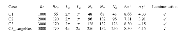
(case C3_LargeBox) using the forcing optimised for the smaller box (case C3). For each Reynolds number, the corresponding forcing term obtained with the ROM-based optimisation was interpolated on the DNS grid. Flow and mesh parameters for the different cases are listed in table 1. Dealiasing is ensured in the DNS by multiplying the number of points in the streamwise and spanwise directions,
 $N_x$
and
 $N_z$
, by a factor of 3/2. The simulations are advanced in time up to
 $t=4000$
, and the forcing term is turned on at
 $t=1500$
and turned off at
 $t=3000$
using a hyperbolic tangent time ramp. This is exactly the same procedure adopted for the ROM simulations described in § 3.
List of parameters for DNS of forced Couette flows. Here,
 $N_x$
,
 $N_y$
and
 $N_z$
are the number of grid points in the streamwise, wall-normal and spanwise directions, respectively,
 $\Delta x^+$
and
 $\Delta z^+$
are the grid spacings in the streamwise and spanwise directions, in wall units and
 $Re_\tau$
is the Reynolds number based on the friction velocity. The values of
 $Re_\tau$
indicated in the second column correspond to a time average computed in the first part of the simulation, when the forcing is off.

Validation of the simulations was made through comparison with existing DNS data from Pirozzoli et al. (Reference Pirozzoli, Bernardini and Orlandi2014) at
 $Re=3000$
(
 $L_x = 18\pi$
,
 $L_z=8\pi$
) and also from Orlandi et al. (Reference Orlandi, Bernardini and Pirozzoli2015) (
 $L_x = 18\pi$
,
 $L_z=8\pi$
) and Lee & Moser (Reference Lee and Moser2018) (
 $L_x = 20\pi$
,
 $L_z=5\pi$
) at higher Reynolds numbers. As discussed above, due to the small domain dimensions and low Reynolds numbers explored here, our simulations do not capture the very-large-scale structures (or extreme-scale motions) reported in those studies. It was shown by Tsukahara et al. (Reference Tsukahara, Kawamura and Shingai2006) that domains larger than
 $L_x \approx 60h, L_z \approx 16h$
are required in order to correctly describe these structures and avoid confinement effects due to the periodic boundary conditions. We have, nevertheless, verified that the near-wall turbulence dynamics is accurately represented in the small domains.
In figure 15, profiles of mean flow and second-order statistics of the C3 and C3_LargeBox cases are compared with data from Pirozzoli et al. (Reference Pirozzoli, Bernardini and Orlandi2014) at the same Reynolds number. Statistics obtained with the ROM are also shown for completeness. Quantities are expressed in wall units,
 $u^+ = u/u_\tau$
,
 $v^+ = v/u_\tau$
,
 $w^+ = w/u_\tau$
,
 $y^+ = (y+1)$
 $u_\tau /\nu$
, and are computed in the first part of the simulation, before the forcing is switched on. The mean-flow profile is given as
 $U^+ = \langle u^+\rangle _{x,z,t}$
, where the symbol
 $\langle \cdot \rangle _{x,z,t}$
denotes averaging in the streamwise and spanwise directions and in time. The friction velocity is defined as
 $u_\tau = \sqrt {\tau _w/\rho }$
, where
 $\tau _w$
is the wall shear stress and
 $\rho$
is the density. Both the mean flow and the Reynolds stresses from the present simulations are in good agreement with the DNS data from Pirozzoli et al. (Reference Pirozzoli, Bernardini and Orlandi2014). The expected peak of
 $\langle uu^+\rangle _{x,z,t}$
at
 $y^{+}=15$
is well captured in the present simulations. However, some degree of discrepancy exists further from the wall, which is expected, since the large-scale structures observed in the larger boxes become dominant further from the wall. This discrepancy is reduced in the C3_LargeBox case. As the box in this case is larger than the spanwise wavenumber of these structures
 $\lambda _z \approx 5h$
(Kitoh et al. Reference Kitoh, Nakabyashi and Nishimura2005; Pirozzoli et al. Reference Pirozzoli, Bernardini and Orlandi2014), they start to develop. This becomes clear in the pre-multiplied energy spectra.
Couette flow statistics at
 $Re=3000$
. (a) Mean-flow profiles; (b) second-order statistics. Solid lines: data from Pirozzoli et al. (Reference Pirozzoli, Bernardini and Orlandi2014); dashed lines: DNS case C3; dash-dotted lines: DNS data from C3_LargeBox; dotted lines: ROM.

Pre-multipled spanwise spectrum,
 $k_z E_{uu}^{+}$
as a function of wall distance,
 $y^+$
. Panel (a) refers to flow case C3 (
 $L_x = 2\pi h, L_z=\pi h$
), and panel (b) refers to flow case C3_LargeBox (
 $L_x = 4\pi h, L_z=2\pi h$
). Dashed lines correspond to data from the present study and solid lines are data from Lee & Moser (Reference Lee and Moser2018) for
 $Re_{\tau }$
,
 $L_x = 20\pi h, L_z=5\pi h$
. The vertical dashed line marks the cutoff wavelength of the present DNS. Nine contour levels are shown, between 0.34 and 3.08.

Figure 16 shows pre-multiplied spanwise spectra of streamwise velocity, computed for the C3 and C3_LargeBox cases and compared with data from Lee & Moser (Reference Lee and Moser2018) for
 $Re_{\tau }=219$
and domain size
 $L_x = 20\pi h, L_z=5\pi h$
. The strong signature of the extreme-scale motions in Lee & Moser’s data is evident around
 $\lambda _z^+ \approx 1147$
(
 $\lambda _z \approx 5.2$
). This is absent in the spectra of the C3 case, due to the small spanwise length of the domain. In the C3_LargeBox case the signature of these structures starts to appear, as can be seen in figure 16(b). The associated spanwise length is, however, smaller than
 $\lambda _z =5h$
, likely due to some confinement effects. Their energy is also small compared with the spectral peak at
 $\lambda_z^{+}=100$
, which shows that larger domains are necessary to fully capture the dynamics of extreme-scale motions typical of Couette flow. However, notice that at smaller wavelengths the data from the present study are in agreement with those of Lee & Moser. Particularly, the spectral peak at
 $y^+ \approx 15, \lambda _z^{+} \approx 100$
associated with the near-wall self-sustaining cycle (Hamilton et al. Reference Hamilton, Kim and Waleffe1995) is well represented. This suggests that the structure of the flow in the small domain is consistent with that of fully developed near-wall turbulence, even though turbulence features in the outer layer are absent. This is further confirmed by the profiles of turbulent kinetic energy production, shown in Appendix C and compared with data from Orlandi et al. (Reference Orlandi, Bernardini and Pirozzoli2015) for higher Reynolds numbers. The agreement in the near-wall region (viscous and buffer layers) is excellent, showing that turbulence production in our data is indeed in agreement with what is expected from fully developed near-wall turbulence at higher Reynolds numbers and larger domains.
Energy budget analysis computed for DNS and ROMs at
 $Re=1000$
, (a),
 $Re=2000$
(b) and
 $Re=3000$
(c). Inputs and dissipation are normalised by the laminar values for Couette flow.

We now turn our attention to the control effect on the full system. At all Reynolds numbers, the flow in the DNS reaches the laminar Couette state upon removal of the forcing, as observed in the ROMs. Laminarisation was also achieved in the larger box through the same mechanisms. Figure 17 shows the energy budget in cases C1, C2 and C3 as a function of time. The data for the corresponding ROMs are also shown for comparison. The temporal evolution of inputs and dissipation in the DNS follow, to a great extent, the same features observed in the ROM. In the first part of the simulations the flow is turbulent, and the shear-driven input,
 $I_1$
and the dissipation,
 $D$
, oscillate intermittently, but are in balance over large time periods. We note that larger oscillations of
 $I_1$
are observed in the ROM compared with the DNS. This is due to the truncation of the ROM. The absence of small scales in the reduced system, which are mainly responsible for the dissipation, interrupts part of the energy cascade. Consequently, a larger portion of the energy remains in the large-scale, energy-producing structures. These take the form of the largest streaks and rolls in the basis, as shown in figure 7. After activation of the forcing, the flow enters a transient period, during which
 $I_1$
decays sharply. The duration of this period is very similar in the ROM and in the DNS at
 $Re=1000$
and
 $2000$
. At
 $Re=300$
the transient is slightly shorter in the ROM. At
 $t \gtrsim 1800$
the dissipation stabilises at a constant value, balancing the energy input provided by the forcing,
 $I_2$
. Finally, the flow reaches the laminar Couette state both in the DNS and the ROMs approximately 300 time units after the forcing is disabled. The energy budget of the C3_LargeBox case was found to be similar to those of the smaller boxes, and is omitted here for conciseness.
In all the simulations the Reynolds number based on the wall velocity,
 $Re$
, is fixed, but the friction Reynolds number fluctuates in time. Time histories of
 $Re_{\tau }$
computed from DNS are displayed in figure 18. Its behaviour is consistent with the energy budgets discussed above: after activation of the forcing it assumes a constant intermediate value associated with the new laminar state and, when the forcing is disabled, it drops to lower second plateau, which corresponds to the Couette laminar values.
Time history of the friction Reynolds number computed from DNS.

Time histories of spatially averaged cross-flow velocities
 $\langle v^2 \rangle$
,
 $\langle w^2 \rangle$
, computed from DNS at
 $Re=1000$
–
 $3000$
.

In order to further investigate the flow regime in the DNS during the application of the forcing, we have computed time histories of the spatially averaged cross-flow velocities
 $\langle v^2 \rangle$
,
 $\langle w^2 \rangle$
, which are displayed in figure 19 in log scale. These provide a direct indication of the persistence of turbulence. At
 $Re=1000$
, as the forced flow is linearly stable,
 $\langle v^2 \rangle$
,
 $\langle w^2 \rangle$
drop almost monotonically after the forcing is turned on,
 $t\gt 1500$
. At
 $Re=2000, 3000$
, on the other hand, the cross-flow velocities initially drop by a few orders of magnitude after the forcing is switched on, but reach an intermediary state, with a clear plateau forming at
 $Re=3000$
. The appearance of an intermediary turbulent state is consistent with the unstable behaviour of the forced base flows at these
 $Re$
, as discussed in Appendix B. But, as also shown in Appendix B using the Orr–Sommerfeld–Squire equations, albeit unstable, the transient amplifications supported by the new laminar states are substantially reduced with respect to that of the canonical Couette laminar flow. This is the same trend observed in the analyses of the linear operator from the ROM, shown in §§ 3.1 and 3.2. Ultimately, transient growth is more important for the dynamics of self-sustaining wall turbulence. In our case, since transient growth is severely inhibited in the forced flow, the low disturbance levels produced by the modal instabilities present in the DNS are unable to sustain a fully turbulent regime or to trigger transition to turbulence upon removal of the forcing. Full relaminarisation is therefore reached after the forcing is disabled.
The mean velocity profiles of the forced flow computed from DNS are displayed in figure 20 for the three cases, and compared with the steady-state solutions obtained from the ROM. As velocity fluctuations are quite low in the forced flow, the mean flows from the DNS are virtually identical to the laminar profiles obtained in the controlled ROMs. This further demonstrates that the control mechanism derived from the reduced system acts in the same manner in the full system. Streamwise velocity profiles taken in the initial transient period after the forcing is switched on,
 $1500 \lesssim t \lesssim 2000$
, were found to evolve smoothly from the turbulent (uncontrolled) mean Couette profile to the forced flow states shown in figure 20. They are omitted here for conciseness.
Laminar flow profiles obtained in the controlled DNS (solid grey lines), compared with the turbulent mean flow (solid black lines) and the laminar flow from the controlled ROMs (dashed line) for cases C1 (a), C2 (b) and C3 (c).

Figure 21 shows three-dimensional snapshots of streamwise velocity taken at selected time instants of DNS and ROM simulations at
 $Re=3000$
. In panels (a) and (f) the flow is turbulent. Panels (b) and (g) are taken shortly after the forcing is applied, and it can be seen that it first disrupts large-scale flow features that meander around the centre of the channel. At
 $t=1600$
(panels (c) and (h)), turbulence still persists at smaller scales close to the walls. However, these scales also die out around
 $t \approx 1800$
, and panels (d) and (i) illustrate how the shear remains confined to the vicinity of the walls. Finally, panels (e) and (j), taken after removal of the forcing, display laminar Couette flow. Movies based on the time evolution of streamwise velocity snapshots throughout the DNS and ROM simulations are provided as supplementary material.
Three-dimensional streamwise velocity snapshots taken from
 $Re=3000$
simulations at selected time instants before, during and after application of the forcing. Panels (a)–(e) correspond to DNS and panels (f)–(j) to ROM simulations. The colours correspond to ten velocity contours, equally spaced in the range
 $-1 \leqslant u \leqslant 1$
.

5. Discussion
As shown above, the control mechanism derived from the ROMs relies on cutting the energy extraction from the sheared laminar flow. For the uncontrolled flow, the energy extraction is mainly carried out by large-scale rolls, which then amplify large-scale streaks via the lift-up mechanism. The strength of this mechanism can be characterised by the maximum transient amplification, which was shown to be substantially reduced in the controlled flow. Reduction of the linear transient growth is a feature observed in other successful control approaches (Kühnen et al. Reference Kühnen, Scarselli, Schaner and Hof2018a
,Reference Kühnen, Song, Scarselli, Budanur, Burak, Riedl, Willis, Avila and Hof
b
; Massaro et al. Reference Massaro, Martinelli, Schmid and Quadrio2023). For pipe flows, this feature has been associated in previous works with the ability of the control strategy to flatten the mean streamwise velocity profile (Kühnen et al. Reference Kühnen, Scarselli, Schaner and Hof2018a
,Reference Kühnen, Song, Scarselli, Budanur, Burak, Riedl, Willis, Avila and Hof
b
; Hof et al. Reference Hof, Lozar, Avila, Tu and Schneider2010; Marensi, Willis & Kerswell Reference Marensi, Willis and Kerswell2019). In the present results, flattening of the velocity profile in the controlled flow is only marked at
 $Re=3000$
(see figure 20). At
 $Re=1000$
and
 $Re=2000$
, the laminar flows display rather an ‘inverted’ shape with respect to the mean turbulent profile (although the absolute velocities are lower in the central part of the channel, as in Kühnen et al. Reference Kühnen, Scarselli, Schaner and Hof2018a
). This indicates that there are other possible ways to manipulate the shape of the velocity profile in order to reduce transient growth. Furthermore, another important difference between the present control strategy and that adopted in Kühnen et al.’s work is that, in their case, the forcing first induces an increase in velocity fluctuations and wall shear stresses; it is only after this first phase that the flow relaminarises, due to the change in the mean turbulent profile. In our case, on the other hand, velocity fluctuations and wall shear stresses drop immediately after the forcing is switched off, either leading the flow to a new laminar state (at
 $Re=1000$
), or to a weak turbulent state (at
 $Re=2000,3000$
), whose associated velocity profiles also inhibit transient growth via the lift-up mechanism.
Furthermore, it is important to emphasise one point about the return of the flow to the laminar uncontrolled state after removal of the forcing. As discussed above, the importance of linear transient growth for the maintenance of a turbulent regime is now well established. In that sense, the linear stability characteristics of the controlled laminar state certainly play a role in inhibiting transition to turbulence when the forcing is switched off. However, transition to turbulence is eminently nonlinear in Couette flow (the laminar profile being linearly stable for all
 $Re$
), and the nonlinear response of the flow to finite-amplitude disturbances is certainly important in determining whether transition to turbulence takes place. Therefore, a full picture of the transition process in the controlled flow involves, ultimately, characterising the basin of attraction of the laminar state and how it is modified by the forcing. There has been significant progress in developing methods to characterise the so-called minimal seed, which is the disturbance with the lowest energy capable of triggering transition to turbulence (Pringle & Kerswell Reference Pringle and Kerswell2010; Pringle, Willis & Kerswell Reference Pringle, Willis and Kerswell2012; Kerswell Reference Kerswell2018). A recent study by Marensi et al. (Reference Marensi, Willis and Kerswell2019) assessed the effect of a steady body force on the critical disturbance energy,
 $E_c$
, for the onset of turbulence, i.e. the energy of the minimal seed, on pipe flows. The body force is designed to mimic the effect of a baffle in the flow, such as that used in Kühnen et al.’s experiments. By tuning the amplitude of the body forcing carefully, they show that it can produce a full collapse of turbulence, pushing
 $E_c \to \infty$
. From a dynamical-systems point of view, this expands the basin of attraction of the laminar state, making it the only global attractor. The results of the robustness analysis shown in figure 13 suggest that a similar trend is produced by the body force considered here. Regardless of how high the amplitudes of the initial disturbances set in the ROM simulations are, when the forcing is applied at the beginning of the simulations the flow is unable to sustain a turbulent state in the presence of the forcing. A rigorous characterisation of
 $E_c$
and the shape of the minimal seed for the present controlled and uncontrolled configurations is, however, outside the scope of this work and is left to future studies.
Finally, a series of numerical experiments by Budanur et al. (Reference Budanur, Marensi, Willis and Hof2020) has shown that transition to turbulence in pipe flows is underpinned by large turbulent energy production away from the wall, in contrast to fully developed turbulent states, in which production is confined to the near-wall region. They suggest that control strategies that aim at preventing transition to turbulence should, therefore, target velocity fluctuations away from the wall. This is consistent with the destruction of large-scale structures in the central part of the channel in our case (figure 21), and it suggests that transition can also be avoided in Couette flow via the same mechanism. Furthermore, it is suggested in the same study that a reduction in linear transient growth can be understood as a proxy for reductions in turbulent energy production away from the wall, which explains the success of Kühnen et al.’s approach in destabilising turbulence. This is also consistent with our findings for Couette flow.
6. Conclusions and perspectives
We have explored a framework for turbulence control in plane Couette flow using a ROM obtained through Galerkin projections with controllability modes. Simulations are performed at Reynolds numbers
 $Re=1000,2000,3000$
in domains with dimensions
 $L_x=2\pi h, L_z=\pi h$
and
 $L_x=4\pi h, L_z=2\pi h$
. Such small domains and low Reynolds numbers preclude the full formation of large-scale structures and extreme-scale motions (Lee & Moser Reference Lee and Moser2018) in the outer flow region. Therefore, the control mechanism derived with the ROMs targets primarily the dynamics of near-wall turbulence, which is found to be consistent with that observed at higher Reynolds numbers and larger domains. Control is provided by a steady body force, linearly expanded in terms of Stokes modes. The expansion coefficients are optimised using a gradient-descent algorithm in order to minimise the total fluctuation energy of the flow. The optimisation was performed over a time horizon divided into two segments: one in which the forcing is active, and a second one in which it is turned off.
The present study brings some contributions from flow physics and methodological points of view. The flow physics aspects concern the mechanisms underlying turbulence suppression in Couette flow through steady forcing, which might also provide useful insights for future turbulence control studies. We show that the optimal forcing affects fundamental mechanisms of near-wall turbulence dynamics, preventing the maintenance of a fully turbulent regime and transition to turbulence when the forcing is removed. Some particular aspects of the control mechanism are worth emphasising. For instance, analysis of the energy budget of the controlled flow reveals that the optimal forcing hinders the main mechanism of turbulent production, which comes from the extraction of energy by the sheared base flow. We show that the production is associated primarily with the largest streaks and rolls in the flow, and, therefore, that the forcing disrupts the self-sustaining turbulence cycle. A control mechanism that completely disrupts the self-sustaining cycle in Couette flow is, to the best of our knowledge, a novelty of our study. Furthermore, the forced flow possesses a new laminar solution, which is linearly stable at
 $Re=1000$
and unstable at higher
 $Re$
. But despite being unstable, the forced flow at
 $Re=2000, 3000$
remains at a state of ‘weak turbulence’, characterised by fluctuation levels which are orders of magnitude below those of the unforced flow. This shows that such instabilities alone are not sufficient to sustain a fully turbulent regime in Couette flow once the control is turned off. This is directly associated with a massive reduction of linear transient growth. Reduction of transient amplification is a feature shared by successful control strategies in other flow geometries, such as pipe (Kühnen et al. Reference Kühnen, Scarselli, Schaner and Hof2018a
,Reference Kühnen, Song, Scarselli, Budanur, Burak, Riedl, Willis, Avila and Hof
b
) and channel (Massaro et al. Reference Massaro, Martinelli, Schmid and Quadrio2023) flows, but this is the first time this has been observed in controlled Couette flow. Furthermore, we show that the control mechanism lowers the maximum transient amplification below the threshold set by the transitional Reynolds number. This effectively prevents the forced flow from sustaining a turbulent regime and explains why, when the forcing is switched off, it fails to transition to a turbulent state, going back to the laminar uncontrolled Couette state.
This mechanism is found to be robust to changes in the shape and amplitude of initial conditions, but its effectiveness is rather sensitive to departures from the design Reynolds number. Moreover, forces optimised in a domain with
 $L_x=2\pi, L_z=\pi$
were also found to be effective in a domain twice this size, in which the signature of large-scale motions starts to appear, albeit with low energy. This suggests a certain robustness of the control mechanism regarding domain dimensions, although it remains to be tested whether this mechanism would be effective in very large domains, where very-large-scale structures become dominant in the outer region.
The methodological aspect concerns the development of a ROM-based method for turbulence control. Our results demonstrate that ROMs can provide an affordable, suitable framework to design and optimise turbulence control strategies. Of particular note is the fact that, despite the high level of truncation of the model, which is apparent in figure 21 and in the supplementary movies, the same control mechanism derived in the ROM is effective in the full system. The forcing optimisation method laid out here might, for instance, be extended to other flow configurations, provided that suitable ROMs exist. Furthermore, there is no fundamental obstacle to extending the optimisation method to higher Reynolds numbers, with the caveat that more modes might need to be included in the ROM basis in order to keep a minimum accuracy. As shown in Appendix A, increasing the Reynolds number with a fixed number of modes inevitably leads to loss of accuracy. Therefore, larger bases need to be used. This can be accomplished either by including more wavenumbers or by increasing the number of controllability modes for each wavenumber pair. The central idea is that the ROM be capable of capturing most of the relevant dynamics at the targeted Reynolds number (ideally with the highest possible truncation) since, ultimately, we want the body forcing designed in the ROM to be effective in the full system.
Furthermore, the forcing adopted in the present study being low-dimensional, computation of the gradient
 $\partial \mathcal{J}/\partial b_j$
as laid out in § 2.1 remains affordable within the ROM framework. But for higher Reynolds numbers and/or different flow configurations, higher-dimensional forcing may be required and, in such cases, adjoint-based optimisation methods might be more appropriate. Combining adjoint-based optimisation with the ROM framework is also an appealing idea, since deriving the adjoint equations for the ROM is much simpler than for the full system. Moreover, here a single initial condition is considered in order to find an optimal forcing, which then turned out to work for different turbulent trajectories. Another possibility is to perform optimisation over an ensemble of turbulent trajectories; this may also be considered in future works, as it might further reinforce the robustness of the control mechanism.
Finally, the forcing structures obtained in this study are not the only possibility allowed in the ROM framework. We can also design body forcings confined to the near-wall region, which could be more easily implemented in experiments. This can be done, for instance, by imposing spatial modulations to the forcing term described in (2.9). The ROMs can, therefore, be used to provide guidance for actuator placement and actuation amplitude. Other forcing principles are also possible with the ROM. One can for instance, apply an unsteady forcing. The simpler case would be a harmonic forcing, in which the frequency is fixed and the same formalism laid out here would be used to optimise the shape and amplitude of the forcing. For more general cases with complex temporal behaviour, such as broadband forcing, the ROM can be coupled with adjoint-based optimisation methods in order to produce a robust mathematical framework. Adaptations of the ROM to include wall-based control, such as spanwise motions or blowing and suction, are also possible, and may provide future directions to design control methods applicable in experiments. In this case, since the forcing is applied at the boundaries of the domain, we can adopt the strategy laid out by Bergmann & Cordier (Reference Bergmann and Cordier2008), wherein the effect of the control is incorporated into a set of actuation modes, which are obtained as particular solutions to the Navier–Stokes equations. The shape and time dependences of these modes can then be subject to an optimisation algorithm in order to minimise a suitable functional, similar to what is done in the present study. Alternatively, the forcing can be designed so as to mimic the effect of a given experimental device. For instance, Marensi et al. (Reference Marensi, Ding, Willis and Kerswell2020) used DNS, combined with an adjoint method, to optimise a forcing term that models the effect of the baffle used in the experiments of Kühnen et al. (Kühnen et al. Reference Kühnen, Scarselli, Schaner and Hof2018a ) to laminarise pipe flows. Similar ideas can be explored within the present ROM-based framework, with the advantage of a major reduction in cost.
Supplementary movies.
Supplementary movies are available at https://doi.org/10.1017/jfm.2025.10258.
Funding.
This work was funded by the São Paulo Research Foundation-FAPESP through Grant No. 2022/06824-4 and by Conselho Nacional de Desenvolvimento Tecnológico-CNPq through Grant No. 314927/2023-9.
Declaration of interests.
The authors report no conflict of interest.
Data availability statement.
The data and codes used to generate the results of the present work may be provided upon reasonable request to the authors.
Appendix A. Flow statistics obtained with different ROMs
Here, we assess the accuracy of the ROM in representing first- and second-order flow statistics. Reduced-order models of different sizes can be obtained by changing the number of wavenumber pairs retained in the basis or the number of controllability modes taken for each wavenumber pairs. Table 2 lists the parameters used to produced ROMs with
 $N=360,600,900$
DoFs. Figures 22 and 23 show mean and r.m.s. velocity profiles obtained with these ROMs, compared with DNS data computed for the same flow conditions. At
 $Re=1000$
the different ROMs display similar accuracy, and all three are in reasonable agreement with DNS. One should keep in mind that perfect agreement with data should not be expected, given the low dimensionality of the chosen ROMs. Furthermore, at a slightly higher Reynolds number (
 $Re=1200$
), the
 $N=600$
ROM was found to correctly describe fundamental aspects of turbulent dynamics, such as inter-scale interactions and self-sustaining processes (McCormack et al. Reference McCormack, Cavalieri and Hwang2024). Therefore, at
 $Re=1000$
this ROM can be considered as a good compromise between compactness and accuracy.
However, at
 $Re=3000$
the two smaller ROMs (
 $N=360,600$
) produce wavy mean velocity profiles characterised by higher deviations from the DNS data. Particularly, the oscillatory behaviour of the mean profile in these ROMS was found to introduce modal instabilities in the controlled flows during the optimisation procedure, a trend which was not observed in the DNS. This undesired effect was corrected with the addition of more controllability modes in the
 $N=900$
ROM. The larger ROM also yields better agreement, overall, regarding the r.m.s. profiles. Therefore, based on these trends, the
 $N=900$
was selected to carry out the forcing optimisations at all the Reynolds numbers considered here.
The accuracy of this ROM in estimating the correct turbulent fluctuating energy can be expressed by a single parameter that represents the error with respect to the turbulent kinetic energy (TKE) obtained from DNS
 \begin{equation} \epsilon = \frac {|| \text{TKE}_{DNS}-\text{TKE}_{ROM}||_2}{||\text{TKE}_{DNS}||_2}, \end{equation}
where
 $||\cdot ||_2$
denotes an
 $l^2$
-norm. Table 3 shows the values of
 $\epsilon$
for
 $Re=1000-$
 $3000$
obtained with the
 $N=900$
ROM. The error increases with Reynolds number, as the model truncation becomes more severe. But despite the relatively high error at the highest
 $Re$
, this may still be found reasonable, considering the degree of reduction attained with the ROM. Furthermore, the forcing mechanism derived in the ROM is still effective in the DNS, suggesting that the ROM preserves essential features of turbulence dynamics.
Parameters of ROMs with different sizes. Here,
 $N_c$
represents the number of controllability modes taken for each wavenumber pair and
 $N$
is the total number of DoFs.

Flows statistics at
 $Re=1000$
obtained with ROMs of different sizes, compared with DNS data. Panels (a), (b), (c) and (d) correspond, respectively, to profiles of mean flow, r.m.s. streamwise velocity, r.m.s. wall-normal velocity and r.m.s. spanwise velocity.

Flows statistics at
 $Re=3000$
obtained with ROMs of different sizes, compared with DNS data. Panels (a), (b), (c) and (d) correspond, respectively, to profiles of mean flow, r.m.s. streamwise velocity, r.m.s. wall-normal velocity and r.m.s. spanwise velocity.

Appendix B. Stability analysis of the full system using the Orr–Sommerfeld–Squire equations
In this section we describe modal and non-modal stability analyses of the full system performed with the Orr–Sommerfeld–Squire equations. We start from the initial-value problem
 \begin{gather} \mathbf{M}\frac {\partial \mathbf{q}}{\partial t} = \mathbf{L}\mathbf{q}, \nonumber\\[5pt] \frac {\partial \mathbf{q}}{\partial t} = \mathbf{M}^{-1}\mathbf{L}\mathbf{q} = \mathbf{L}_1\mathbf{q}, \end{gather}
Error in estimation of TKE levels by the
 $N=900$
ROM at different Reynolds numbers.

where
 $\hat {\mathbf{q}} =( \hat {v} \ \hat {\eta })^{T}$
is a vector containing the wall-normal velocity and the wall-normal vorticity
 \begin{equation} \eta = \frac {\partial u}{\partial z} - \frac {\partial w}{\partial x}. \end{equation}
Matrices
 $\mathbf{M}$
and
 $\mathbf{L}$
are defined as
 \begin{equation} \begin{aligned} \begin{gathered} \mathbf{M} = \left (\begin{array}{c c} k^2-\mathcal{D}^2 & 0\\ 0 & 1\\ \end{array}\right) \\[4pt] \mathbf{L} = \left (\begin{array}{c c} \mathcal{L}_{OS} & 0\\[4pt] ik_z U^{\prime} & \mathcal{L}_{SQ}\\ \end{array}\right), \end{gathered} \end{aligned} \end{equation}
where
 $\mathcal{D}$
is a wall-normal differentiation operator, and the Orr–Sommerfeld and Squire operators are given as,
 \begin{align} \mathcal{L}_{OS} & = ik_x U \big( k^2-\mathcal{D}^2 \big) + ik_x U^{\prime\prime} + \frac {1}{\textit{Re}}\big( k^2-\mathcal{D}^2 \big)^2, \nonumber\\ \mathcal{L}_{SQ} & = ik_x U + \frac {1}{\textit{Re}} \big( k^2-\mathcal{D}^2 \big), \end{align}
where
 $k^2 = k_x^2 + k_z^2$
,
 $U$
is the streamwise-and-spanwise-independent base flow and the
 $^{\prime}$
and
 $^{\prime\prime}$
symbols denote first- and second-order derivation, respectively. Assuming solutions of the form
 $\mathbf{q} = \hat {\mathbf{q}} \ \text{exp}(-i \omega t)$
, the initial-value problem can be recast as an eigenvalue problem
 \begin{equation} \mathbf{L} \hat {\mathbf{q}} = -i \omega \mathbf{M}\hat {\mathbf{q}}. \end{equation}
Linear stability of the forced laminar state for the wavenumber pairs described in the ROM, computed with the Orr–Sommerfeld–Squire equations for
 $Re=1000, 2000, 3000$
. Panels (a)-(d) show eigenvalue spectra for four wavenumber pairs: (a)
 $(k_x/\alpha, k_z/\beta) = (0,1)$
; (b)
 $(k_x/\alpha, k_z/\beta) = (0,2)$
; (c)
 $(k_x/\alpha, k_z/\beta) = (1,1)$
; (d)
 $(k_x/\alpha, k_z/\beta) = (1,2)$
.

A modal stability analysis can then be performed by solving this eigenvalue problem. Stability/instability of the system is then determined by the imaginary part of the eigenvalues,
 $\omega _i$
. It is well known that the laminar Couette flow is linearly stable for all Reynolds numbers. Therefore, here, we focus on modal stability of the forced base flows. Figure 24 shows eigenvalue spectra computed for the three forced base flows obtained from the ROM and the DNS (which were shown to be identical) at
 $Re=1000, 2000, 3000$
. The spectra were computed for four wavenumber pairs:
 $(k_x/\alpha, k_z/\beta)=(0,1)$
,
 $(k_x/\alpha, k_z/\beta)=(0,2)$
,
 $(k_x/\alpha, k_z/\beta)=(1,1)$
and
 $(k_x/\alpha, k_z/\beta)=(1,2)$
. The domain was discretised with a Chebyshev grid, and we found that
 $N=180$
points were sufficient to attain converged results. Dirichlet boundary conditions were applied for
 $\hat {v}$
and
 $\hat {\eta }$
at
 $y \pm 1$
; Neumann boundary conditions are also imposed on
 $\hat {v}$
. All modes computed for these wavenumbers combinations are stable (
 $\omega _i\lt 0$
).
Furthermore, we have also assessed the stability of the forced base flows for a range of streamwise wavenumbers not contained in the ROM, and to a range of Reynolds numbers. The forced base flow obtained at
 $Re=1000$
was found to be linearly stable for all wavenumbers and Reynolds numbers tested. At
 $Re=2000$
and
 $Re=3000$
, on the other hand, the base flows were found to be unstable in a broad region of the
 $k_x$
-
 $Re$
plane. Figure 25 shows neutral stability curves computed for two-dimensional disturbances,
 $k_z=0$
. The forced base flows obtained at
 $Re=2000$
and
 $Re=3000$
are found to be unstable even at the design Reynolds numbers, with the unstable modes possessing streamwise wavenumbers higher than those contained in the ROM (
 $k_x/\alpha \gt 2$
). Such instabilities are related to the inflection points of the base flows at
 $Re=2000$
and 3000, which are related to shear layers with low velocity differences that nonetheless display the typical Kelvin–Helmholtz instability. The neutral curve for
 $Re=3000$
has a more complex shape, as up to five unstable modes are found for the studied
 $k_x-Re$
combinations. The instability at the design Reynolds numbers is consistent with the ‘weak’ turbulent state observed when the forcing is active (see figures 19
b and 19
c). Furthermore, the broad region of instability at higher Reynolds numbers is likely associated with the lack of robustness of the forcing to changes in
 $Re$
.
Neutral stability curves computed for the forced base flows obtained at
 $Re=2000$
(a) and
 $Re=3000$
(b). The corresponding spanwise wavenumber is fixed,
 $k_z=0$
. The shaded area corresponds to the region in the
 $k_x$
–
 $Re$
space where unstable solutions exist.

Non-modal stability, on the other hand, can be analysed by the transient growth supported by the base flow. For that we have used eigenfunction expansions (Schmid & Henningson Reference Schmid and Henningson2012). This technique consists in expanding the vector functions,
 $\mathbf{q}$
, into the basis
 $\{\hat {\mathbf{q}}_1, \ldots,\hat {\mathbf{q}}_N \}$
, which represents the space
 $\mathbb{S}^{N}$
spanned by the first
 $N$
eigenfunctions of
 $\mathbf{L}_1$
 \begin{equation} \hat {q} = \sum _{n=1}^{N}\kappa _n(t)\hat {\mathbf{q}}_n \qquad \qquad \hat {\mathbf{q}} \in \mathbb{S}^{N}. \end{equation}
Transient growth curves for the laminar Couette flow and the laminar state of the forced flow, computed with the Orr–Sommerfeld–Squire equations for four wavenumber pairs: (a)
 $(k_x/\alpha, k_z/\beta) = (0,1)$
; (b)
 $(k_x/\alpha, k_z/\beta) = (0,2)$
; (c)
 $(k_x/\alpha, k_z/\beta) = (1,1)$
; (d)
 $(k_x/\alpha, k_z/\beta) = (1,2)$
. The inset in panel (a) shows a zoomed view of the curves corresponding to controlled cases. Legend is the same as in figure 11.

The initial-value form can then be rewritten in the simpler form
 \begin{equation} \frac {\text{d}\kappa }{\text{d}t} = -i \Lambda \kappa \quad \quad \quad \Lambda \in \mathbb{C}^{N \times N} \quad \quad \quad \kappa \in \mathbb{C}^{N}, \end{equation}
with
 $\kappa = (\kappa _1, \kappa _2, \ldots, \kappa _N)^{T}$
and
 $\Lambda = \text{diag}\{\omega _1, \omega _2, \ldots, \omega _N\}$
. The temporal evolution of disturbances is then described by the evolution of the expansion coefficients,
 $\kappa _n$
, instead of
 $\mathbf{q}$
. In order to complete this transformation, the inner product needs to be reformulated in term of the expansion coefficients. For
 $\hat {q}_1, \hat {q}_2 \in \mathbb{S}^{N}$
we define
 \begin{equation} (\mathbf{q}_1,\mathbf{q}_2)_{E} = \frac {1}{k^2}\int _{-1}^{1} \mathbf{q}_2^H\mathbf{M}\mathbf{q}_1\text{d}y = \kappa _2^HM\kappa _1, \end{equation}
where the symbol
 $H$
stands for the Hermitian transpose, and the matrix
 $M$
is given by
 \begin{equation} M_{ij} =(\hat {\mathbf{q}}_i,\hat {\mathbf{q}}_j)_E = \frac {1}{k^2}\int _{-1}^{1}\hat {\mathbf{q}}_j^H\mathbf{M}\hat {\mathbf{q}}\text{d}y. \end{equation}
Here,
 $M$
is both Hermitian and positive definite, and therefore it can be factored into
 $M = F^HF$
. Finally, the maximum possible amplification of any initial state is given as
 \begin{equation} \begin{aligned} G(t) =& \max _{q_{0}^{\prime} \neq 0} \frac {||\mathbf{q}(t)||_{E}^2}{||\mathbf{q}_0||_{E}^2}\\ =& ||F \ \text{exp}(-i t \Lambda) \ F^{-1}||_{E}^2\\ =& \sigma _1^2 (F \ \text{exp}(-i t \Lambda) \ F^{-1}), \end{aligned} \end{equation}
with
 $\sigma _1$
the leading singular value. We performed this analysis considering both the laminar Coeuette and the forced Couette velocity profiles as base flows, considering wavenumbers typical of streaky structures involved in the transition of laminar Couette flow; for these wavenumbers, both velocity profiles are linearly stable. The analysis was carried out for the same wavenumber pairs considered in the modal analysis, and using the same discretisation and boundary conditions. The inner products are computed with discrete versions of equations (B8) and (B9) using Clenshaw–Curtis quadrature weights. As discussed in Maia & Cavalieri (Reference Maia and Cavalieri2024), flow structures with
 $(k_x/\alpha, k_z/\beta)=(0,1)$
correspond to the largest streak/roll pairs, which are also the most controllable modes in the ROM basis. Modes with
 $k_x \neq 0$
correspond to oblique waves associated with streak instabilities. Transient growth curves are displayed in figure 26. For all wavenumber pairs, transient growth of the forced Couette state is substantially reduced with respect to the standard laminar Couette base flow. Furthermore, the peak values of
 $G(t)$
remain almost constant in the forced case, irrespective of the Reynolds number, whereas they increase with Reynolds number for the laminar Couette flow. The largest amplifications are associated with the largest streaks,
 $(k_x/\alpha, k_z/\beta)=(0,1)$
. Notice that the transient growth curves shown in figure 26(a) are quite similar to those computed using the linearised operators of the ROM. This indicates that the transient growth behaviour of the flow is controlled, to a large extent, by the non-modal growth of these structures.
Appendix C. Turbulent kinetic energy production
In this section we present the turbulent kinetic energy production,
 $P^{+} = -\langle u^{\prime}v^{\prime} \rangle ^{+}\text{d}\langle U \rangle ^{+}/\text{d}y^{+}$
, computed from the DNS and compared with data from Orlandi et al. (Reference Orlandi, Bernardini and Pirozzoli2015) at higher Reynolds numbers. They have shown that turbulent production in the near-wall region of Couette flow is almost independent of Reynolds number. Here, we assess whether this trend remains consistent in small domains such as ours. Wall-normal profiles of
 $P^+$
are displayed in figure 27. The data from the present study are in excellent agreement with Orlandi et al.’s data. The peak in production at
 $y^+ \approx 10$
region is well matched, further showing that the dynamics of near-wall turbulence in the small box is consistent with that observed in larger boxes and much higher Reynolds numbers, even at the lowest Reynolds number explored.
Profiles of turbulent kinetic energy production. The solid lines correspond to data from the present study: C1 (red); C2 (blue); C3 (black). The symbols are data from Orlandi et al. (Reference Orlandi, Bernardini and Pirozzoli2015) for different Reynolds numbers:
 $Re_{\tau }=180$
(squares),
 $Re_{\tau }=250$
(circles),
 $Re_{\tau }=500$
(triangles) and
 $Re_{\tau }=1000$
(downward-pointing triangles).