1. Introduction
1.1. Context
Bubbles are important in many geophysical, biological and industrial settings. Whether exsolving from magma (Sparks Reference Sparks1978), scavenging surface-active bacteria in the ocean (Blanchard Reference Blanchard1989) or forming the head on a pint of beer, bubble–bubble coalescence influences the size distribution and consequent effects. Coalescence and film rupture are also of intrinsic interest as fundamental processes associated with free-surface singularities. Here, we consider the case of coalescence of two initially static and spherical bubbles.
An important parameter for the generic case of drop coalescence in an outer fluid is the ratio
 ${\it\lambda}$
of the inner-fluid viscosity to the outer-fluid viscosity. Hopper (Reference Hopper1984) derived an analytic solution in two dimensions for the case
 ${\it\lambda}=\infty$
(coalescence of drops with an inviscid exterior) using complex-variable methods for Stokes flow, while Paulsen et al. (Reference Paulsen, Burton, Nagel, Appathurai, Harris and Basaran2012) argued that this solution is changed by the inertia of the drops at any non-zero Reynolds number. The intermediate case of finite non-zero
 ${\it\lambda}$
is a free-boundary problem which can be approached with computational methods (Leal Reference Leal1990) or at early times with asymptotic methods for viscous flow (Eggers, Lister & Stone Reference Eggers, Lister and Stone1999). At later times or lower viscosities, inertia plays a role (e.g. Aarts et al.
Reference Aarts, Lekkerkerker, Guo, Wegdam and Bonn2005; Burton & Taborek Reference Burton and Taborek2007). The work described here is distinct from these studies in that it is concerned with the case
 ${\it\lambda}=0$
.
Bubbles start to coalesce when the fluid sheet between them is ruptured, and surface tension acting on the edge of the resulting hole causes the sheet to retract and the hole to grow; the resistance from the viscosity and inertia of the sheet determines the rate of growth. There is a rich history of work on rupture and retraction of fluid sheets. Taylor and Culick independently modelled the flow as a sheet with an inviscid cylindrical rim, moving with a velocity that they found to be
 $(2{\it\gamma}/{\it\rho}h)^{1/2}$
for a sheet of uniform thickness
 $h$
, density
 ${\it\rho}$
and surface tension
 ${\it\gamma}$
(Taylor Reference Taylor1959; Culick Reference Culick1960). Keller extended their ideas to the rupture of inviscid fluid sheets with non-uniform thickness (Keller Reference Keller1983). Further numerical simulations, analytical studies and experiments have explored the effects of viscosity on sheet rupture, and shown that sufficiently high viscosity can prevent formation of a rim (Debrégeas, Martin & Brochard-Wyart Reference Debrégeas, Martin and Brochard-Wyart1995; Brenner & Gueyffier Reference Brenner and Gueyffier1999; Savva & Bush Reference Savva and Bush2009).
Recent images of the early stages of bubble coalescence by Paulsen et al. (Reference Paulsen, Carmigniani, Burton and Nagel2014) showed that the radius of the hole at time
 $t$
grows proportional to
 $t^{1/2}$
for any viscosity of the outer fluid. They observed that the rate of coalescence has one scaling in the case of a high-viscosity outer fluid, and another scaling in the case of low viscosity. Although a scaling argument was given for these two limiting regimes, it was based on scalings that we show here do not always capture the true thickness and radial extent of the perturbed portion of the fluid sheet. In particular, the solution for the case of low Ohnesorge number
 $\mathit{Oh}$
(i.e. low viscosity) has a length scale much shorter than the radius of the hole by a factor of
 $\mathit{Oh}$
. Remarkably, we show that for general
 $\mathit{Oh}$
the initially quadratic sheet profile permits a similarity solution in which the ratio of viscous and inertial effects is independent of time. Linear or uniform sheet profiles do not admit such a similarity solution (Billingham Reference Billingham2005; Savva & Bush Reference Savva and Bush2009) unless viscosity or inertia is neglected (e.g. Keller & Miksis Reference Keller and Miksis1983; Ting & Keller Reference Ting and Keller1990; Miksis & Vanden-Broeck Reference Miksis and Vanden-Broeck1999; Sierou & Lister Reference Sierou and Lister2004).
1.2. Problem overview
Consider two spherical bubbles of equal radius
 $a$
and take cylindrical polar coordinates
 $(r,z)$
with the axis aligned through the centres of the spheres (see figure 1). Let the external fluid between the bubbles have density
 ${\it\rho}$
, dynamic viscosity
 ${\it\mu}$
and velocity components
 $u$
and
 $w$
in the radial and axial directions respectively. We assume that the system is axisymmetric for all time, so that the azimuthal velocity is zero. We define the Ohnesorge number by
 $\mathit{Oh}={\it\mu}/({\it\rho}a{\it\gamma})^{1/2}$
, where
 ${\it\gamma}$
is the (constant) coefficient of surface tension. We neglect the viscosity of the fluid inside the bubbles, and treat the pressure there as constant, which we may set equal to zero. We consider the case where the two bubbles are brought together sufficiently slowly that coalescence begins essentially at the point of geometrical contact between spherical bubbles.
Schematic section through the axisymmetric problem, showing the fluid sheet exterior to the bubbles of thickness
 $h$
and the velocity components
 $u$
and
 $w$
in the radial and axial directions respectively. The edge of the sheet has radial position
 $r_{\!E}$
and thickness
 $h_{E}$
(see text).

Just before coalescence, the thickness of the fluid sheet for
 $r\ll a$
is thus approximately
 $r^{2}/a$
, which is much less than the radial coordinate
 $r$
. Hence, the sheet is initially long and thin, and we will assume that it remains long and thin through the early stages of coalescence, while shortening and thickening as the edge of the sheet retracts. Let
 $r_{\!E}(t)$
be the radial position of the edge of the sheet. Then, near
 $r_{\!E}$
, surface tension acting in the
 $(r,z)$
plane smooths the edge of the sheet into a rounded tip over a radial extent proportional to the thickness
 $h_{E}$
of the edge of the sheet. In this region, which is small if
 $h_{E}\ll r_{\!E}$
, the sheet is locally not long and thin, but we can match the solution for a long thin sheet to a local solution for the rounded tip. This structure is a two-dimensional analogue of that described by Eggers (Reference Eggers2014) for a retracting viscous thread, matching a slender-thread solution to a rounded finger in Stokes flow.
The asymptotic equations of motion for the system are developed in § 2, put in self-similar form, and then solved numerically in § 3. For comparison, the full Navier–Stokes equations were simulated numerically. The calculations identify two limiting regimes, as in Paulsen et al. (Reference Paulsen, Carmigniani, Burton and Nagel2014), and the asymptotic structure of the similarity solution in each regime is determined in § 4. Finally, § 5 discusses the self-consistency of this solution, and estimates the time scale over which this early stage of coalescence could be observed.
2. Equations of motion
As the bubbles are inviscid, the fluid sheet is bounded by shear-free surfaces. Since the fluid sheet is long and thin, it may be described by the radial form of the extensional-flow equations, the main ideas of which are sketched below. The fluid velocity is dominantly in the radial direction and, at leading order, is a function only of
 $r$
and
 $t$
. The outward mass flux together with conservation of mass gives
 $$\begin{eqnarray}\frac{\partial h}{\partial t}=-\frac{1}{r}\frac{\partial }{\partial r}(ruh).\end{eqnarray}$$
Balancing the normal stress on the surface of the sheet, which is to leading order
 ${\it\sigma}_{zz}$
, with the capillary pressure gives the pressure in the fluid as
 $$\begin{eqnarray}p=-{\it\gamma}{\it\kappa}-2{\it\mu}\frac{\partial w}{\partial z}=-{\it\gamma}{\it\kappa}+2{\it\mu}\left(\frac{u}{r}+\frac{\partial u}{\partial r}\right),\end{eqnarray}$$
where the second equality follows from local mass conservation and
 ${\it\kappa}$
is the surface curvature of the fluid sheet. Then, balancing the radial components of the hoop stress, the radial viscous stress and the capillary force acting on an arc of fluid with its acceleration gives a leading-order momentum equation
 $$\begin{eqnarray}\underbrace{{\it\rho}h\frac{\text{D}u}{\text{D}t}}_{\text{Inertia}}=\underbrace{{\it\gamma}h\frac{\partial {\it\kappa}}{\partial r}}_{\text{Capillary}}+\underbrace{\frac{2{\it\mu}}{r}\frac{\partial }{\partial r}\left[rh\left(\frac{u}{r}+2\frac{\partial u}{\partial r}\right)\right]}_{\text{Radial stress}}\underbrace{-\frac{2{\it\mu}h}{r}\left(2\frac{u}{r}+\frac{\partial u}{\partial r}\right)}_{\text{Hoop stress}},\end{eqnarray}$$
which agrees with results derived more formally elsewhere (e.g. Savva & Bush Reference Savva and Bush2009; Pegler & Worster Reference Pegler and Worster2012).
The kinematic boundary condition at the edge of the sheet simply means that the radial velocity there must be equal to the velocity of the edge of the sheet. The capillary force from the rounded tip, which is
 $2{\it\gamma}$
per unit azimuthal length to leading order, is supported by the radial viscous stress in the sheet as the hoop stress and inertia are negligible at the edge of the sheet (see appendix). The boundary conditions on the edge of the sheet are therefore
 $$\begin{eqnarray}u(r_{\!E},t)=\frac{\text{d}r_{\!E}}{\text{d}t}\quad \text{and}\quad 2{\it\gamma}=-{\it\gamma}h{\it\kappa}(r_{\!E},t)-2{\it\mu}h\left.\left(\frac{u}{r}+2\frac{\partial u}{\partial r}\right)\right|_{r_{\!E}}.\end{eqnarray}$$
Prior to coalescence at
 $t=0$
, the fluid is static and its thickness is given by the gap between two touching spheres. Hence,
 $$\begin{eqnarray}h(r,t)\rightarrow \frac{r^{2}}{a},\quad u(r,t)\rightarrow 0\quad \text{as }t\rightarrow 0^{+}\text{ at fixed }r.\end{eqnarray}$$
At early times, the curvature at the edge of the sheet is to leading order
 $2/h$
, which is much larger than the curvature
 $h_{rr}$
away from the edge since
 $h\ll r$
, and so the surface-curvature term
 ${\it\gamma}h{\it\kappa}$
in (2.4b
) is negligible. Thus, the dominant balance is between the capillary pressure from the rounded tip and the viscous stress. With this balance, the capillary term in (2.3) is also negligible. We non-dimensionalise the physical variables using scales motivated by the boundary conditions (2.4a
), (2.4b
) and (2.5a
), which give
 $u\sim r/t$
,
 ${\it\gamma}\sim {\it\mu}hu/r$
and
 $h\sim r^{2}/a$
respectively. The remaining terms in (2.3) are all proportional to
 $t^{-1/2}$
(the neglected capillary term is proportional to
 $t^{1/2}$
), and we deduce that the variation
 $h\propto r^{2}$
in the original thickness of the sheet allows for a similarity solution in which inertia and viscosity are in balance for all time (a uniform fluid sheet, a fluid wedge or a cone would not admit such similarity). We define similarity variables
 $$\begin{eqnarray}r=\left(\frac{a{\it\gamma}t}{{\it\mu}}\right)^{1/2}{\it\eta},\quad h=\frac{{\it\gamma}t}{{\it\mu}}H({\it\eta}),\quad u=\left(\frac{a{\it\gamma}}{{\it\mu}t}\right)^{1/2}U({\it\eta}).\end{eqnarray}$$
Equations (2.1) and (2.3) become ordinary differential equations
 $$\begin{eqnarray}\displaystyle & \displaystyle H^{\prime }=H\left(\frac{\displaystyle 1+U^{\prime }+\frac{U}{{\it\eta}}}{\displaystyle \frac{{\it\eta}}{2}-U}\right), & \displaystyle\end{eqnarray}$$
 $$\begin{eqnarray}\displaystyle & \displaystyle \frac{1}{4\mathit{Oh}^{2}}\left(-\frac{1}{2}U-\frac{1}{2}{\it\eta}U^{\prime }+UU^{\prime }\right)=U^{\prime \prime }+\frac{U^{\prime }}{{\it\eta}}-\frac{U}{{\it\eta}^{2}}+\frac{H^{\prime }}{H}\left(U^{\prime }+\frac{U}{2{\it\eta}}\right), & \displaystyle\end{eqnarray}$$
 ${\it\eta}$
. The boundary conditions become
 $$\begin{eqnarray}\displaystyle & \displaystyle U({\it\eta}_{E})=\frac{{\it\eta}_{E}}{2}\quad \text{and}\quad -\frac{1}{H({\it\eta}_{E})}=\frac{U({\it\eta}_{E})}{{\it\eta}_{E}}+2U^{\prime }({\it\eta}_{E}), & \displaystyle\end{eqnarray}$$
 $$\begin{eqnarray}\displaystyle & \displaystyle \frac{H}{{\it\eta}^{2}}\rightarrow 1,\quad {\it\eta}U\rightarrow 0\quad \text{as }{\it\eta}\rightarrow \infty , & \displaystyle\end{eqnarray}$$
where
 ${\it\eta}_{E}$
is the dimensionless position of the edge of the sheet, and (2.9d
) follows from (2.5b
) after eliminating
 $t$
between (2.6a
) and (2.6c
). This third-order system of equations has two boundary conditions at
 ${\it\eta}_{E}$
and two boundary conditions at infinity, which also determine the unknown
 ${\it\eta}_{E}$
.
In order for
 $H$
to be finite at
 ${\it\eta}_{E}$
, (2.7) and (2.9a
) require the regularity condition
 $1+U^{\prime }+U/{\it\eta}=0$
, where
 ${\it\eta}/2=U$
at
 ${\it\eta}_{E}$
. We deduce that
 $U^{\prime }({\it\eta}_{E})=-3/2$
from (2.9a
) and
 $H({\it\eta}_{E})=2/5$
from (2.9b
). This gives the dimensionless thickness of the fluid sheet where it matches to the rounded tip.
For all finite values of
 $\mathit{Oh}$
, there is an asymptotic solution for a far-field region defined by
 $U\ll {\it\eta}$
and
 $U^{\prime }\ll 1$
. Under these conditions, (2.8) reduces at leading order to
 $$\begin{eqnarray}U^{\prime \prime }+\left(\frac{3}{{\it\eta}}+\frac{{\it\eta}}{8\mathit{Oh}^{2}}\right)U^{\prime }+\frac{1}{8\mathit{Oh}^{2}}U=0,\end{eqnarray}$$
which, subject to (2.9d ), has the closed-form solution
 $$\begin{eqnarray}U=A\text{e}^{-{\it\eta}^{2}/(16\,Oh^{2})}F\!\left(\frac{3}{2},2,\frac{{\it\eta}^{2}}{16\mathit{Oh}^{2}}\right),\end{eqnarray}$$
where
 $A$
is a free parameter and
 $F$
is the confluent hypergeometric function of the second kind. For
 ${\it\eta}\gg \mathit{Oh}$
,
 $U\sim A(4\mathit{Oh}/{\it\eta})^{3}\text{e}^{-{\it\eta}^{2}/(16\,Oh^{2})}$
. For the case
 $\mathit{Oh}=\infty$
, or for
 $1\ll {\it\eta}\ll \mathit{Oh}$
, (2.11) is dominated by the viscous terms and
 $U\sim A(2{\rm\pi}^{-1/2})(4\mathit{Oh}/{\it\eta})^{2}$
.
We note that (2.7), (2.8) and (2.9c ) can be combined to show that
 $$\begin{eqnarray}\int _{{\it\eta}_{E}}^{\infty }\frac{\displaystyle U^{\prime }+\frac{3U}{{\it\eta}}}{\displaystyle \frac{{\it\eta}}{2}-U}\text{d}{\it\eta}=\int _{{\it\eta}_{E}}^{\infty }\left(\frac{H^{\prime }}{H}-\frac{2}{{\it\eta}}\right)\text{d}{\it\eta}=\left[\log \left(\frac{H}{{\it\eta}^{2}}\right)\right]_{{\it\eta}_{E}}^{\infty }=\log \left(\frac{5{\it\eta}_{E}^{2}}{2}\right),\end{eqnarray}$$
where the last equality uses the condition
 $H({\it\eta}_{E})=2/5$
. This gives a direct relationship between
 ${\it\eta}_{E}$
and the velocity profile
 $U({\it\eta})$
, which is independent of
 $H^{\prime }$
and
 $H$
.
3. Numerical solution
Equations (2.7) and (2.8) were solved numerically by shooting from the asymptotic behaviour (2.12) towards the boundary conditions
 $U={\it\eta}/2$
and
 $H=2/5$
at
 ${\it\eta}={\it\eta}_{E}$
. We initialised the integration at
 ${\it\eta}\gg \mathit{Oh}$
with the far-field conditions (2.12) and
 $H={\it\eta}^{2}$
, and integrated through decreasing values of
 ${\it\eta}$
until
 $U={\it\eta}/2$
. The free parameter
 $A$
in (2.12) was adjusted to search for the solution with
 $H({\it\eta}_{E})=2/5$
.
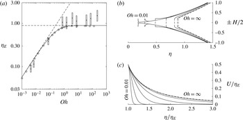
Figure 2(a) shows the values of
 ${\it\eta}_{E}$
calculated in this way for a range of
 $\mathit{Oh}$
similar to the experiments of Paulsen et al. (Reference Paulsen, Carmigniani, Burton and Nagel2014). The experimental data points are also shown, with boxes indicating error bars; Paulsen et al. (Reference Paulsen, Carmigniani, Burton and Nagel2014) give a range for
 ${\it\gamma}$
and report uncertainties in the values of their time scale
 ${\it\tau}_{out}$
which here lead to uncertainty in both
 $\mathit{Oh}$
and
 ${\it\eta}_{E}$
under the similarity scalings. The numerical similarity solutions show the same trends as the experimental data. In particular, we see two limiting regimes with
 ${\it\eta}_{E}\sim 1.807\mathit{Oh}^{1/2}$
for
 $\mathit{Oh}\ll 1$
and
 ${\it\eta}_{E}\sim 0.8908$
for
 $\mathit{Oh}\gg 1$
.
(a) Solid line: numerical solution for
 ${\it\eta}_{E}$
from the similarity equations. Circles: numerical estimation of
 ${\it\eta}_{E}$
from the full Navier–Stokes simulations. Points: experimental data from Paulsen et al. (Reference Paulsen, Carmigniani, Burton and Nagel2014), with boxes indicating error bars. Dashed lines: asymptotic theory for the limits
 $\mathit{Oh}\ll 1$
and
 $\mathit{Oh}\gg 1$
calculated in § 4. (b) Similarity thickness profiles
 $H({\it\eta})$
for
 $\mathit{Oh}=0.01$
, 0.03, 0.1, 0.3, 1 and 3, and for the limit
 $\mathit{Oh}=\infty$
as calculated in § 4.2. (c) Velocity profiles
 $U({\it\eta})$
for the same values of
 $\mathit{Oh}$
, with
 ${\it\eta}$
and
 $U$
both scaled by
 ${\it\eta}_{E}$
.

The thickness and velocity profiles in figure 2(b,c) show that the solution for
 $\mathit{Oh}\gg 1$
is to leading order independent of
 $\mathit{Oh}$
, and for
 $\mathit{Oh}\gtrsim 0.1$
the thickness increases monotonically away from
 ${\it\eta}_{E}$
. However, for
 $\mathit{Oh}\ll 1$
the sheet thins rapidly from
 $H=2/5$
at the edge to
 $H\approx {\it\eta}_{E}^{2}$
over a length scale even smaller than
 ${\it\eta}_{E}$
before increasing again in the far field. Rescaling
 $({\it\eta}-{\it\eta}_{E})$
by
 ${\it\eta}_{E}^{3}$
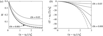
collapses these thickness profiles onto a universal curve as
 $\mathit{Oh}$
decreases (figure 3
a). From (2.9a
),
 $U\approx {\it\eta}_{E}/2$
near
 ${\it\eta}_{E}$
and scaling the small difference
 $(U-{\it\eta}_{E}/2)$
by
 ${\it\eta}_{E}^{3}$
shows a similar collapse towards a universal curve (figure 3
b). Ahead of this short length scale, the velocity is negligible and the thickness is close to
 ${\it\eta}^{2}$
, and within this short length scale, the velocity is
 ${\it\eta}_{E}/2$
to leading order and the thickness is
 $O(1)$
. Therefore, the structure for
 $\mathit{Oh}\ll 1$
is a thickened toroidal ring expanding and sweeping up fluid that is otherwise at rest, with all of the mass in the ring moving at essentially the speed of the edge of the sheet. We note that, even though the ring has a short radial length scale in the similarity solutions, the dimensional solutions are still long and thin for sufficiently early times, as
 $h\propto t$
,
 $r\propto t^{1/2}$
by (2.6a,b
).
Solid lines showing the numerical similarity solutions for
 $\mathit{Oh}=0.001$
, 0.003, 0.01 and 0.03, and dashed lines showing the asymptotic limit for
 $\mathit{Oh}\rightarrow 0$
found in § 4.1. (a) The thickness and (b) the velocity difference with
 $({\it\eta}-{\it\eta}_{E})$
and
 $(U-{\it\eta}_{E}/2)$
each scaled by
 ${\it\eta}_{E}^{3}$
.

The coalescence of two identical bubbles was also simulated numerically by solving the full Navier–Stokes and continuity equations in the fluid exterior to the bubbles. In these simulations, the bubbles were initially two unit-radius spheres connected by a small cylindrical bridge of radius
 $R_{0}$
and half height
 $Z_{0}$
, and the exterior fluid was quiescent. Typical values were
 $R_{0}=10^{-3}$
and
 $Z_{0}=10^{-6}$
, which are sufficiently small that the effects of initial transients decay quickly, and the subsequent dynamics is virtually unchanged if smaller values of
 $R_{0}$
and
 $Z_{0}$
are used. The values of
 ${\it\eta}_{E}$
in figure 2(a) were estimated from a power-law fit over the range
 $0.003\leqslant r_{\!E}\leqslant 0.03$
.
Kinematic and dynamic boundary conditions are imposed on the free surfaces of the bubbles. A stress-free outer boundary condition is imposed on a large sphere enclosing a volume of fluid around the bubbles. The free-boundary problem comprising the Navier–Stokes and continuity equations, together with boundary and initial conditions, is solved numerically by a fully implicit method of lines (MOL) algorithm and an arbitrary Lagrangian–Eulerian (ALE) scheme. The algorithm uses the Galerkin/finite-element method for spatial discretisation and adaptive time stepping. The large interfacial and domain deformations that accompany coalescence are captured by using an elliptic mesh-generation scheme developed by Christodoulou & Scriven (Reference Christodoulou and Scriven1992) for coating flows and later extended to study both drop breakup and coalescence (Notz, Chen & Basaran Reference Notz, Chen and Basaran2001; Notz & Basaran Reference Notz and Basaran2004; Paulsen et al. Reference Paulsen, Burton, Nagel, Appathurai, Harris and Basaran2012). Advantage is taken of both the axisymmetry and the up–down symmetry of the geometry to reduce the computational cost. Additional details of the method and simulations will be provided in a future publication.
The results from simulations of the full Navier–Stokes equations give excellent agreement with the similarity solution for
 ${\it\eta}_{E}$
across the range of
 $\mathit{Oh}$
, which strongly suggests that the terms neglected in the thin-sheet modelling in § 2 are indeed small.
4. Asymptotic solutions for
 $\mathit{Oh}\ll 1$
and
$\mathit{Oh}\gg 1$


4.1.
$\mathit{Oh}\ll 1$

Figures 2 and 3 show evidence of a boundary-layer structure with rapid variations near
 ${\it\eta}_{E}$
over a shorter
 $O({\it\eta}_{E}^{3})$
length scale. A balance of the highest-derivative term
 $U^{\prime \prime }$
in (2.8) with the large advection terms, each scaling as
 ${\it\eta}_{E}U^{\prime }/(4\mathit{Oh}^{2})$
, motivates introduction of a rescaled radial coordinate
 $x=({\it\eta}-{\it\eta}_{E})/L$
, where
 $L=4\mathit{Oh}^{2}/{\it\eta}_{E}$
, and
 $L$
is
 $O({\it\eta}_{E}^{3})$
or
 $O(\mathit{Oh}^{3/2})$
as expected.
Since
 $U$
varies from
 ${\it\eta}_{E}/2$
to 0, it might seem reasonable to make the rescaling
 $V=U/{\it\eta}_{E}$
throughout the boundary layer. However, one must take care with the term
 $({\it\eta}/2-U)^{-1}$
in (2.7). Since
 $U={\it\eta}/2$
at
 ${\it\eta}={\it\eta}_{E}$
from (2.9b
), there is a region near the edge of the sheet where the appropriate rescaling is instead
 ${\it\omega}=(U-{\it\eta}_{E}/2)/L$
.
We eliminate
 $H^{\prime }/H$
between (2.7) and (2.8), switch to the rescaled variables
 $V(x)$
and
 ${\it\omega}(x)$
appropriate to each region, and take the dominant terms to obtain
 $$\begin{eqnarray}\displaystyle & \displaystyle -\frac{1}{2}V_{x}+VV_{x}=V_{xx}+\frac{V_{x}^{2}}{\left(\frac{1}{2}-V\right)}\quad \text{where }({\it\eta}/2-U)\sim {\it\eta}_{E},\quad \text{and} & \displaystyle\end{eqnarray}$$
 $$\begin{eqnarray}\displaystyle & \displaystyle -\frac{1}{4}={\it\omega}_{xx}+\frac{\left({\it\omega}_{x}+\frac{3}{2}\right)\left({\it\omega}_{x}+\frac{1}{4}\right)}{\left(\displaystyle \frac{x}{2}-{\it\omega}\right)}\quad \text{where }({\it\eta}/2-U)\sim L. & \displaystyle\end{eqnarray}$$
Equation (4.1) has a one-parameter family of sigmoidal solutions obeying the boundary condition (2.9d
) given by
 $V=(1+\text{e}^{x/2+b})^{-1}/2$
and parametrised by
 $b$
. As
 $V\rightarrow 1/2$
, the generic behaviour of these solutions is
 $V=(1-\text{e}^{x/2+b})/2$
. The solution for the thickness in this region is
 $H={\it\eta}_{E}^{2}(\text{e}^{-x/2-b}+1)$
.
The substitution
 ${\it\omega}=z(x)+x/2$
makes (4.2) autonomous, and a phase-plane analysis reveals a node at
 $z=0$
,
 $z_{x}=-2$
, which corresponds to the boundary and regularity conditions
 $U({\it\eta}_{E})={\it\eta}_{E}/2$
,
 $U^{\prime }({\it\eta}_{E})=-3/2$
. The trajectories from this node give a one-parameter family of solutions to (4.2), whose generic behaviour as
 ${\it\omega}\rightarrow -\infty$
has the exponential form
 ${\it\omega}=-\text{e}^{kx+c(k)}$
parametrised by
 $k$
, where
 $c(k)$
is an
 $O(1)$
constant.
Therefore, the inner behaviour of solutions to (4.1) matches the outer behaviour of solutions to (4.2) if
 $k=1/2$
and
 $b=c(1/2)+\log (2L/{\it\eta}_{E})$
. We find
 $c(1/2)\approx 1.473$
by numerically integrating (4.2) inwards from a point with
 $-{\it\omega}\gg 1$
and
 ${\it\omega}_{x}={\it\omega}/2$
. With
 $U$
determined, calculating the mass integral (2.13) gives
 ${\it\eta}_{E}\approx 1.807\mathit{Oh}^{1/2}$
. The velocity near
 ${\it\eta}_{E}$
, scaled by
 ${\it\eta}_{E}^{3}$
, in the limit
 $\mathit{Oh}\ll 1$
is shown with a dashed line in figure 3(a). Now that we have the solution for
 $U$
, we may integrate (2.7) to obtain the thickness
 $H$
, and this completes the solution. Under the approximation
 $U={\it\eta}_{E}/2+L{\it\omega}$
, this gives the profile shown in figure 3(b). Figure 3 shows convergence of the numerical solutions towards the asymptotic limits, confirming that the asymptotic structure presented is that of the calculated thickness and velocity profiles. It should be noted that
 $H=O(1)$
only where
 $U={\it\eta}_{E}/2+O(\mathit{Oh}\,r_{\!E})$
. This justifies the structure observed in § 3 of a toroidal ring sweeping up fluid as it advances, as we have shown that where the sheet thickness is perturbed from
 ${\it\eta}^{2}$
, the fluid is moving almost with the velocity of the edge of the sheet.
4.2.
$\mathit{Oh}\gg 1$

In the viscous limit
 $\mathit{Oh}\gg 1$
, neglecting the inertial terms gives the Stokes-flow equation
 $$\begin{eqnarray}U^{\prime \prime }+\frac{U^{\prime }}{{\it\eta}}-\frac{U}{{\it\eta}^{2}}+\left(\frac{\displaystyle 1+U^{\prime }+\frac{U}{{\it\eta}}}{\displaystyle \frac{{\it\eta}}{2}-U}\right)\left(U^{\prime }+\frac{U}{2{\it\eta}}\right)=0.\end{eqnarray}$$
The generic far-field behaviour of (4.3) for
 ${\it\eta}\gg 1$
is
 $U\sim U_{\infty }+U_{0}{\it\eta}^{-2}$
. However, (2.11) shows that inertia plays a role at large distances, where
 ${\it\eta}=O(\mathit{Oh})$
and the solution is the hypergeometric function (2.12). The re-entry of inertia at large distances is analogous to the Oseen correction to Stokes flow at large distances from a moving body. The hypergeometric function has leading-order behaviour
 $U\sim 32A\mathit{Oh}^{2}{\rm\pi}^{-1/2}{\it\eta}^{-2}$
for
 ${\it\eta}\ll \mathit{Oh}$
, which matches the far-field behaviour of (4.3) for
 ${\it\eta}\gg 1$
, provided that
 $U_{\infty }=0$
.
Equation (4.3) was solved by integrating from the far-field behaviour
 $U\sim U_{0}{\it\eta}^{-2}$
to a point with
 $U={\it\eta}/2$
. Instead of shooting with the free parameter
 $U_{0}$
, the solution with
 $U_{0}=1$
can simply be rescaled, as (2.7), (4.3) and the boundary conditions (2.9a,c,d
) are invariant under
 ${\it\eta}\rightarrow {\it\lambda}{\it\eta}$
,
 $U\rightarrow {\it\lambda}U$
,
 $H\rightarrow {\it\lambda}^{2}H$
. Hence, if
 $\tilde{H}$
is the height at
 ${\it\eta}_{E}$
for the solution to (4.3) with
 $U_{0}=1$
, then choosing
 ${\it\lambda}^{2}=0.4/\tilde{H}$
gives the solution that also satisfies boundary condition (2.9b
). This procedure gives
 ${\it\eta}_{E}=0.8908$
and
 $U_{0}=0.3085$
, as shown in figure 2.
5. Conclusions and discussion
We have shown that when two bubbles coalesce, the retraction of the thin sheet of fluid between them is described at early times by a similarity solution with both inertia and viscous stress in balance. This similarity solution is characterised by the Ohnesorge number
 $\mathit{Oh}$
, and exhibits limiting regimes in which the edge of the sheet retracts as
 $$\begin{eqnarray}r_{\!E}=0.8908\left(\frac{a{\it\gamma}}{{\it\mu}}\right)^{1/2}t^{1/2}\quad \text{if }\mathit{Oh}\gg 1\quad \text{or}\quad r_{\!E}=1.807\left(\frac{a{\it\gamma}}{{\it\rho}}\right)^{1/4}t^{1/2}\quad \text{if }\mathit{Oh}\ll 1.\end{eqnarray}$$
The spatial structure of the flow depends on
 $\mathit{Oh}$
, with a new dimensionless radial scale
 $L\sim {\it\eta}_{E}^{3}\ll {\it\eta}_{E}$
if
 $\mathit{Oh}\ll 1$
. The condition for the solution to describe a slender flow is therefore
 $h_{E}\ll r_{\!E}$
if
 $\mathit{Oh}\gtrsim 1$
, but
 $h_{E}\ll \mathit{Oh}\,r_{\!E}$
if
 $\mathit{Oh}\ll 1$
. In the simpler case
 $\mathit{Oh}\gtrsim 1$
, the flow is slender for times
 $t\ll {\it\mu}a/{\it\gamma}$
, after which
 $r_{\!E}\sim a$
and the surface relaxes to a sphere of radius
 $2^{1/3}a$
. However, for
 $\mathit{Oh}\ll 1$
, the flow is slender only for times
 $t\ll \mathit{Oh}^{3}{\it\mu}a/{\it\gamma}$
, at which time the sheet has only retracted to
 $r_{\!E}\sim \mathit{Oh}^{2}a$
, and the retracting rim has thickened into an annular ‘blob’ of thickness
 $h_{E}$
and radial extent
 $L$
, both
 ${\sim}\mathit{Oh}^{3}a$
.
This structure resembles that of an idealised purely inviscid blob model written down ab initio in a short insightful paper by Keller (Reference Keller1983). Keller assumed that all of the fluid from
 $r<r_{\!E}(t)$
collects in an expanding ring of volume
 ${\rm\pi}r_{\!E}^{4}/2a$
and that it moves with uniform velocity
 $\text{d}r_{\!E}/\text{d}t$
. If the only force on the ring is assumed to be surface tension
 $2{\it\gamma}$
acting radially over a length
 $2{\rm\pi}r_{\!E}$
then a radial momentum balance gives
 $$\begin{eqnarray}\frac{\text{d}}{\text{d}t}\left(\frac{{\rm\pi}{\it\rho}r_{\!E}^{4}}{2a}\frac{\text{d}r_{\!E}}{\text{d}t}\right)=4{\rm\pi}{\it\gamma}r_{\!E},\quad \text{with solution}~r_{\!E}=\left(\frac{32a{\it\gamma}}{3{\it\rho}}\right)^{1/4}t^{1/2}.\end{eqnarray}$$
Since
 $(32/3)^{1/4}=1.8072\dots ,$
we see that this simple inviscid model can now be supported at early times by the detailed asymptotic and numerical solutions to the full similarity equations presented here. In particular, we note that the asymptotic separation of the regions described by (4.2) and (4.1) justifies the approximation that (almost) all of the mass of the ring moves with velocity
 $\text{d}r_{\!E}/\text{d}t$
: we found that
 $u=(\text{d}r_{\!E}/\text{d}t)(1+O(\mathit{Oh}))$
where
 $h\sim h_{E}$
, but the large velocity gradient between the moving ring and the undisturbed sheet occurs where
 $h\ll h_{E}$
. Radial viscous stresses play an important role in the gradient region, accelerating the fluid from rest through a short compressional boundary layer as the ring approaches it. The hoop stresses are negligible because the radial velocity gradients are much larger than the azimuthal gradients. Moreover, we anticipate that Keller’s description continues to apply once the ring is no longer slender, but has thickened into an annular blob. Continued accumulation would give a blob of size
 $O(r_{\!E}^{3/2}/a^{1/2})$
by conservation of mass, intermediate between
 $r_{\!E}$
and the local thickness of the sheet
 $r_{\!E}^{2}/a$
. Velocity variations and viscous stresses will be important only in a relatively small volume at the junction, and so the rate of coalescence will still be described by
 $r_{\!E}=(32a{\it\gamma}/(3{\it\rho}))^{1/4}t^{1/2}$
. In fact, the full Navier–Stokes simulations for
 $\mathit{Oh}\ll 1$
were initialised with
 $r\gg \mathit{Oh}^{2}a$
and demonstrate coalescence in this regime.
There are some small differences between the theoretical results presented here and the experimental results of Paulsen et al. (Reference Paulsen, Carmigniani, Burton and Nagel2014). This may be because current imaging techniques make it difficult to capture very early-time evolution with
 $r_{\!E}$
much smaller than
 $10^{-1}a$
. Moreover, the initial conditions of the theory require the bubbles to be perfectly spherical and for the fluid to be at rest, whereas in reality the bubbles must be moved together by some force at some velocity and there will be some draining flow between the bubbles. This may deform the bubbles, although with the bubbles brought together sufficiently slowly, the deformation can be limited to a small region (Davis, Schonberg & Rallison Reference Davis, Schonberg and Rallison1989). If the deformation flattens the bubbles near contact then the local curvature is reduced, the effective value of
 $a$
in (2.5a
) is increased, and the entire solution could be adapted for that value of
 $a$
to give a faster rate of coalescence.
Given the idealised initial conditions, the excellent agreement between the similarity solutions and the full Navier–Stokes simulations shows that the approximations of § 2 give a full understanding of the essential dynamics of the problem.
Acknowledgements
J.P.M. acknowledges an Engineering and Physical Sciences Research Council studentship. C.R.A. and O.A.B. acknowledge the Donors of the American Chemical Society Petroleum Research Fund for partial support of this research. All data accompanying this publication are directly available within the publication.
Appendix. The rounded tip
The thin-sheet similarity equations (2.7)–(2.9) predict that the fluid sheet ends with non-zero thickness
 $h_{E}=(2{\it\gamma}t/5{\it\mu})$
at its retreating edge
 $r=r_{\!E}(t)$
. Capillary forces must act locally to smooth this edge into a rounded tip, which we argue occurs over a radial length scale comparable to
 $h_{E}$
. For sufficiently early times, since
 $h_{E}\propto t$
and
 $r_{\!E}\propto t^{1/2}$
, the length scale of the rounded tip is much smaller than the length scale
 $r_{\!E}$
of velocity and thickness variations in the sheet. (For
 $\mathit{Oh}\ll 1$
the length scale in the sheet is actually
 $\mathit{Oh}\,r_{\!E}$
not
 $r_{\!E}$
, but this detail does not affect the argument.) Hence, for the rounded tip to match onto the thin sheet on an intermediate length scale between
 $h_{E}$
and
 $r_{\!E}$
, the asymptotic thickness and velocity of the rounded tip solution must match the thickness and velocity of the edge of the sheet, and the forces must also match.
Consider the radial component of the forces acting on an arc of the rounded tip over an azimuthal extent
 $\text{d}{\it\theta}$
and radial extent
 $O(h_{E})$
. (Or
 $O(t^{{\it\alpha}})$
with
 $1/2<{\it\alpha}<1$
.) The radial force from surface tension is
 $2{\it\gamma}r_{\!E}\text{d}{\it\theta}\propto t^{1/2}$
. The viscous stresses scale with
 ${\it\mu}u/r_{\!E}\propto t^{-1}$
(again taking
 $r_{\!E}$
as the scale of velocity variations for simplicity). The radial stress acts on the join of the arc to the sheet, which has area
 $h_{E}r_{\!E}\text{d}{\it\theta}\propto t^{3/2}$
, to give a force
 $\propto t^{1/2}$
; the hoop stress acts on the ends of the arc, which have area proportional to
 $h_{E}^{2}\propto t^{2}$
(and inclination
 $\text{d}{\it\theta}$
), to give a force
 $\propto t$
. The rate of change of momentum of the arc is proportional to
 ${\it\rho}h_{E}^{2}r_{\!E}\,\text{d}{\it\theta}u/t\propto t$
. At early times, therefore, the force balance on the tip is dominated by the radial stress and surface tension, and the effects of hoop stress and inertia are negligible. We conclude that the matching condition to the thin-sheet equations is indeed the boundary condition (2.4b
).
We also conclude that the tip solution is asymptotically that of a two-dimensional sheet retracting in Stokes flow and tending to uniform thickness
 $h_{E}$
; it is similar to the viscous solution in Brenner & Gueyffier (Reference Brenner and Gueyffier1999), but with an additional negative contribution to the pressure from the term
 $u/r$
in (2.4b
). The detailed analysis is closely analogous to the similarity solution of Eggers (Reference Eggers2014) for an axisymmetric retracting finger in Stokes flow. In summary, there is a similarity solution to the Stokes equations in a two-dimensional sheet of the form
 $\boldsymbol{u}(\boldsymbol{x},t)=(2{\it\gamma}/5{\it\mu})(U(X,Z),Y/2,W(X,Z))$
,
 $h(x,t)=h_{E}(t)\mathscr{H}(X)$
, where
 $h_{E}(t)=2{\it\gamma}t/5{\it\mu}$
,
 $(X,Y,Z)=(x,y,z)/h_{E}$
, with
 $U\sim -3X/2$
,
 $W\sim Z$
and
 $\mathscr{H}\rightarrow 1$
as
 $X\rightarrow \infty$
, and
 $\boldsymbol{u}(\mathbf{0})=\mathbf{0}$
and
 $\mathscr{H}(0)=0$
. This solution, with a suitable choice of translating origin, forms the asymptotic ‘inner’ tip solution and matches to the ‘outer’ thin-sheet solution. We have not needed to solve these two-dimensional Stokes equations numerically, since the correction to
 $r_{\!E}(t)$
due to the rounded tip is only
 $O(h_{E})$
and is therefore negligible at early times.