“REFORMATTING” CENTRAL EUROPE: THE PARIS PEACE TREATIES AND AFTER

Maps 1 and 2 document the dramatic shifts in state boundaries brought about by the Great War and the postwar settlements, especially so with regards to Central and East-Central Europe. Most significantly, the Habsburg Empire was broken up, its territories divided between several independent successor states and neighboring countries. German territorial and population losses, though considerable, were modest in comparison to those inflicted on Austria, Hungary, Bulgaria, and Russia. Poland was resurrected as a sovereign nation state and refashioned from lands that since the Partitions of Poland (1772–1795) have been under Habsburg, Hohenzollern, and Romanov rule. Germany lost most of the Prussian provinces of Posen and of West Prussia, and the eastern part of Upper Silesia, whilst Austria ceded Galicia, with an ethnically very diverse population, to the new Polish state that also incorporated the formerly Russian Kingdom of Poland and other eastern territories annexed from Russia and Lithuania. Czechoslovakia was created from regions previously under Austrian (Bohemia, Moravia, and Silesia) and Hungarian (Slovakia and Carpathian Ruthenia) rule and was to include large German and Hungarian minorities which, together, made up more than a quarter of the new state's population. Yugoslavia was formed from the union of former Habsburg lands (Croatia-Slavonia, Slovenia, Bosnia, and Hercegovina) with Serbia and, later, Montenegro. Romania's territorial acquisitions included Transylvania from Hungary, Bessarabia from Russia, the Dobrudja from Bulgaria, and the Bukovina from Austria.

MAP 1

EUROPE 1914

Notes: The map shows the political borders in Central Europe in 1914.Source: Smitha, maps from http://www.fsmitha.com/h2/, 2004.

MAP 2

EUROPE 1921

Notes: The map shows the political borders in Central Europe in 1921.Source: Smitha, maps from http://www.fsmitha.com/h2/, 2004.

Although territorial change and new state formation started before the Paris Peace Conferences of 1919/20, and continued thereafter as in the case of the Polish-Russian War that ended with the 1921 Treaty of Riga, the main outlines of the postwar map of Central Europe were put down in Versailles, St. Germain, and Trianon. Initially, the victorious powers attempted to reshape the region after 1918 along the lines of President Wilson's Fourteen Points,Footnote ⁹ partly to promote new states’ legitimacy and democracy, and partly to provide a cordon sanitaire against Soviet Russia and Germany. The victors proclaimed “national self-determination,” as a key principle whose intent was to put Central Europe on a path towards Western-type democracies.Footnote ¹⁰ The territorial section of the peace conference noted that “frontiers should be drawn as far as possible on ethnic lines.”Footnote ¹¹ That is, “nation states” were to be defined first and foremost in terms of ethnicity. However, and perhaps unsurprisingly, the very notion of national “self-determination” proved deeply problematic when confronted with Central Europe's ethnically heterogeneous settlement patterns. Different nationalities often shared the same territories and even classifying individuals into “ethnic” groups was difficult and controversial.Footnote ¹² Moreover, the national movements in Central Europe attempted to maximize the political and economic power of their new states, which resulted in numerous territorial disputes, for example, between Poles and Czechs over railways or between Poles and Germans over access to the sea.Footnote ¹³ The doctrine of national self-determination had a political fatal flaw: it asserted that borders in Central and East-Central Europe should (and could) be drawn “in accordance with historically established lines of allegiance and nationality.” This, Robert Bideleux and Ian Jeffries argue, effectively ignored that in this part of Europe “nations and nationalities were relatively recent mental constructs, which were not even based on uniformly applicable criteria.Footnote ¹⁴ They were variously defined in terms of ‘national’ language or ‘national’ religion or common territory or shared history or dynastic allegiance.” Whichever way the borders would be drawn, one nation's gain and “justice” were often another's loss and “injustice.”

How did the new, post-1918 borders come about? The historiography on the peace settlement is extensive and diverse, but it points to several factors that governed postwar border changes. Poland was an exception since the Allies had agreed to resurrect the state during the war, albeit crucially without agreement on its eventual boundaries.Footnote ¹⁵ For the rest of Central Europe, matters evolved over time. President Wilson did not intend to establish new borders there when he argued for the principle of national self-determination in his famous Fourteen Points of January 1918. For the case of Austria-Hungary, he rather envisaged a multinational federation within the old boundaries, a position supported by the British government until mid-1918.Footnote ¹⁶ Events on the ground and in particular the strength of independence movements of the nations that had lived under Habsburg rule rendered that plan moot. By the time the Paris Peace Conferences started, Czechoslovakia's existence, for example, had already been recognized by the Allies and it controlled most of the territories it wanted.Footnote ¹⁷ The redrawing of Central Europe's map—before, during, and even after the conferences—was a messy process where historical claims on territory, geographical, and strategic concerns as well as claims for ethnic homogeneity of states’ populations clashed. Poland illustrates the profound dilemmas faced by the Peacemakers of 1919/20. Wilson had initially envisaged that it would include those territories that are “indisputably Polish.” This could be taken to mean, either, giving the Polish state its widest historical extent, thus including a large number of non-Poles. It could also be taken to restrict Poland to the “heartlands,” leaving large numbers of Poles outside the new state.Footnote ¹⁸ Neither definition really implemented national self-determination. Eventually, Helga Schultz argues, “an ethnic principle was established for the Polish state.”Footnote ¹⁹ Other countries were designed using different metrics, and the evidence on the principles shaping the process of border changes is far from conclusive. On balance, though, Schultz maintains “economic arguments tended to come third, after history and nationality” in the process of redrawing state boundaries in Central and Eastern Europe.Footnote ²⁰ Nevertheless, for our purposes we cannot take the borders to have been drawn randomly.

How the state boundaries of Central Europe were drawn remains obscure, we also know rather less about the effect of these new borders on Europe's economies than we would like. During the interwar, a host of mainly German or Austrian publications argued that the new borders had dismembered well-integrated economic areas, with devastating consequences for trade and production.Footnote ²¹ This remains conventional wisdom in the modern literature.Footnote ²² However, the only serious attempt to trace the effects of new borders on trade with the statistical tools available in the interwar years, comes to a surprising result: “[In] the rebuilding of European integration after the war only gradual dislocations occurred, which in no way altered the fundamental equilibrium within European trade relationships.”Footnote ²³ This motivates the key questions of our article: Did the Paris Peacemakers manage to redraw the European map with many new states but with limited damage to trade? Did the new borders reflect the prewar patterns of trade because they followed ethnic, geographical, historical, or other lines of fragmentation?

A NEW DATA SET ON CENTRAL EUROPE'S REGIONAL TRADE FLOWS, 1885–1933

This study draws on a new data set that documents the exports of 31 into 43 Central European regions before and after World War I. To measure trade flows, the data set covers six years, three (1885, 1910, and 1913) before and three (1925, 1926, and 1933) after the First World War. All border changes in these regions occurred between 1919 and 1921, hence well after 1913 and well before 1925. Due to chaotic circumstances including war, revolution, and hyperinflation, data for the period 1914–1924 are either unavailable or unusable. We focus on railway shipments (accounting for about 85 percent of total trade of the region) of seven commodity groups which represent a wide array of sectors of the economy. They include rye—an important agricultural product; brown coal and hard coal—natural resources used for power generation in industry and transport and for domestic heating, as well as coke, which is a key input in ironmaking and steelmaking. Furthermore, the data set covers three groups of processed industrial products: iron and steel (semi-) manufactures, cardboard and paper products, and chemical products. In total, we have about 50,000 observations of flows of one of these products for a year from one region of Central Europe to another.

The main data sources are two series of annual railway statistics. The first, the Statistik der Güterbewegung auf Deutschen Eisenbahnen (Statistics of the Movement of Goods on German Railways) runs from 1885 to 1914.Footnote ²⁴ After the war, the German Statistical Office published nearly identical series through the 1930s. These series document railway shipments between all parts of Germany in 1914 borders—split into 27 transport districts (TD)—and shipments between them and 16 European neighboring countries or regions. We extended this data set significantly by adding commodity-specific railway shipments of three districts covering the Habsburg Empire (or its successor states, respectively) and of the Kingdom of Poland. Before 1914 this involved reconstructing trade flows for the Russian Kingdom of Poland and the different regions of the Habsburg Empire. For Russian Poland, we used the railway and customs data compiled by Henryk Tennenbaum in his Bilans Handlowy Królestwa Polskiego (The Trade Balance of the Kingdom of Poland).Footnote ²⁵ Although some efforts towards national statistics were undertaken in various parts of the multinational Habsburg state, only Hungary (Transleithania) produced usable trade statistics. Here we relied on A Magyar Szent Korona Országainak 1882–1913. Évi Külkereskedelmi Forgamla (Foreign Trade of the Lands of the Holy Hungarian Crown, 1882–1913)—a foreign trade statistics based on railway shipments. For the Austrian half of the empire (Cisleithania), trade flows have been reconstructed in a two-stage process. First, data on trade in mining products (brown coal, hard coal, coke) were taken directly from the official Austrian Bergbaustatistik which documents not only regional production levels, but also shipments from one region to another within Cisleithania and abroad (including Hungary). Second, for all other goods covered in this study, Austrian trade with non-German districts was isolated using the official foreign trade statistics of the Austro-Hungarian customs union (Waren-Ausfuhr; Statistik des auswärtigen Handels) and subtracting the flows to and from Hungary (from the Hungarian foreign trade statistics), Bohemia, and Galicia (from a range of sources). Internal (i.e., intra-district) trade was approximated by subtracting regional exports from regional output.Footnote ²⁶

After 1918 the statistical administrations which were quickly set up in all of the newly formed independent states in Central Europe provide the needed data. Detailed railway statistics are available for Poland and the Saargebiet with geographical definitions of TDs that are almost identical to the ones used in the German statistics. Moreover, we used the official commodity-specific trade statistics of Poland, Czechoslovakia, Hungary, Austria, and the statistics of the French départements of Bas-Rhin, Haut Rhin, and Moselle.

We focus on 43 transport districts.Footnote ²⁷ For 31 transport districts (27 German in the prewar borders, three Habsburg, and one Russian), we have internal (that is intra-district) shipments as well as data on their exports to and imports from all other TDs. This gives us a total of 1,333 export shipments per year and traded good.Footnote ²⁸ All data are given in metric tons. Shipments of less than 0.5 tons were documented as zero in all statistics. Map 3 shows the districts location.

The railway data we use have some important features: they involve shipments by rail between regions of final destination (excluding transits). The shipment data is well-suited to exploring economic integration between regions within states as it represents by far the largest share of total trade flows in Central Europe. The share of railways in total trade was quite constant across our sample at about 85 percent, with some variation between regions but little over time.Footnote ²⁹ Whenever a shipment from region A to C was sent via region B, this is documented as shipment from A to C as long as the shipment is on railways only. In the case of a change in transport mode (for example, if goods are first shipped by railway from A to B and then by waterway from B to C), the shipment data would imply a bias, especially towards trade hubs, such as ports. Data for 1913 suggests that this was an issue, because 20 percent of all railway shipments in hard coal and 11 percent of shipments in grains either originated or ended at an inland or seaport.Footnote ³⁰ However, note that the new borders were drawn in regions that lacked major waterways, with the exception of Alsace-Lorraine, where the new border largely followed the Rhine. We will explain in the next section how our estimation method can take this issue into account.

MAP 3

CONSOLIDATED TRADE DISTRICTS OF CENTRAL EUROPE

Notes: See footnote 27 for a list of trade districts; bold black lines indicate new state borders that were not present prior to 1914. The light grey districts are part of Germany after 1918. We have full data on shipments within and between all the light grey shaded districts and the dark grey shaded districts no. 2, 8, 21, 29, 30, 32, and 34 (a total of 31). In addition, we have data on railway shipments between these 31 and the remaining 12 districts.

Our sources document trade flows at the substate level for Germany and her neighbors. For example, the Habsburg Empire is covered in three TDs that, together, include four major regions: Galicia is enumerated with Bukovina, Hungary includes Croatia-Slavonia, Slovakia, and Bosnia, meanwhile Bohemia, comes with Austria and Moravia. Unfortunately, before 1914 Austria and Bohemia are counted together, except for rye and hard coal. Therefore, we pool the two together throughout but run robustness checks with the more disaggregated data for rye and hard coal. Importantly, shipments from and into the Kingdom of Poland are also reported separately from those of the Russian Empire (of which it was a part). Moreover, the geographical definition of German and foreign TDs prior to the war matches very closely the demarcation of new countries after the First World War. While we lack detailed information on this issue, the definition of TDs apparently followed quite closely preexisting administrative units. Finally, after 1919 the Weimar authorities continued to rely on the same trade districts as before the war. This is a most remarkable feature of the data set. For example, for the postwar Republic of Poland, the sources distinguish between “East Poland” (the former Russian part), “West Poland” (the former German part except Upper Silesia), “East Upper Silesia,” and “Galicia” (the former Austrian part). Similarly, shipments to and from Alsace-Lorraine were reported separately from those relating to France even after 1919. These unique features allow us to trace regional trade flows across Central Europe over the whole period 1885–1933, despite the profound changes in political-administrative borders.

ANALYTICAL APPROACH: IDENTIFYING THE TREATMENT EFFECT OF BORDERS

Ideally, one would like to compare trade flows at time t between two regions i and j separated by a border with trade flows at time t between two identical regions i and j, but not separated by a border (the control group). The difference in trade flows would be the “treatment effect” of that border on trade. However, we never observe identical pairs of regions at time t with and simultaneously without a border. Empirical studies have relied on a gravity model to produce a control group. In this case, trade flows at time t between region pairs separated by a border are compared to trade flows at time t between regions pairs not separated by a border after controlling for regional characteristics and some basic pairwise characteristics. However, we can never rule out that there is some unobserved pairwise heterogeneity, not captured by the gravity model that essentially drives the estimated border effects. Thus it is not clear whether it is actually the treatment effect of borders on trade that has been estimated or the effects of some other factors that just happen to vary along that border, such as, for example, the effects of ethnolinguistic networks or natural geography.

Our solution is to assume that the unobserved pairwise heterogeneity is fixed over time and use a difference-in-difference estimator. We compare the difference in the difference of trade flows over time between two regions i and j without a border to that of regions k and l between which there is a border. The first set of differences (in the cross-section) accounts for unobservable pairwise heterogeneity, the second accounts for the treatment (changes over time). Most often one cannot observe trade flows between two regions i and j both before and after border is put in place, because national statistical systems, including for example the definition of regions and commodity groups change, together with changes borders. However, the new data set exploited here removes this major constraint.

Difference-in-difference (DD) estimators are widely used to assess the treatment effect of a policy.Footnote ³¹ Here we estimate the treatment effect of borders on trade with a DD estimator in levels, as suggested by Orley Ashenfelter and Ashenfelter and David Card and Albrecht Ritschl and Nikolaus Wolf.Footnote ³² We implement this estimator within the framework of the now standard micro-founded formulation of a gravity model on trade flows from Anderson and van Wincoop,Footnote ³³ modified for our historical data. Following their approach, at any point in time exports X from region i to j in a certain period can be explained by the relative economic size of the exporter and the importer and on the bilateral resistance to trade (denoted by “t,” which is “one” plus the tariff equivalent of trade barriers) between them. Anderson and van Wincoop show that trade resistance needs to be expressed relative to the overall barriers to trade of the respective trading partners, i.e., in terms of “bilateral resistance” relative to inward “multilateral resistance” P and outward “multilateral resistance” Φ.Footnote ³⁴ The elasticity of substitution between varieties of k from different exporters i is denoted by σ. The gravity model is then formulated as (for good k)

(1)

The variables in equation 1 are not directly observable. However, except for trade costs they are region-specific, but not pair-specific, so one can consistently estimate the average effect of trade costs on the flow of goods by introducing two sets of time-varying dummies for each region and product class k, namely A_i^k_,t and A_j^k_,t.Footnote ³⁵ These dummy variables are equal to one whenever a region enters the equation as an importer or exporter, respectively. In general, the model requires trade flows in values whereas our data involve tons of good shipped. Following Anderson and van Wincoop, we assume trade costs to be proportional in trade values or that, where Z^k_ij is the volume of exports in metric tons.Footnote ³⁶ We can move to quantities Z because each price p_i^k is exporter-specific and thus absorbed by the respective (time-varying) exporter dummy. Therefore, we replace the unknown terms in equation 1 with time-varying exporter A_i^{k ’} effects (that now include price effects p_i^k) and importer A_j^k effects (again dropping the time index).

(2)

In equation 2, C is a constant, and the importer and exporter specific dummies capture all region-specific heterogeneity. Importantly, these dummies also take into account the fact that inland ports and seaports will generate much higher railway traffic than other regions. This will limit the possible bias implied by the fact that our data is restricted to railway shipments.Footnote ³⁷ The variable t^k_ij denotes again one plus the tariff equivalent of bilateral trade barriers, which are the main focus of our study.

To analyze these barriers, we have to make some further assumptions about trade costs (t^k_ij). We assume they increase (i) with distance, which we proxy by a linear function of geographical distances dist, (ii) when crossing existing political borders as well as (iii) when crossing prospective political borders. We are agnostic about why trade costs might rise when there are no formal borders. All we want is to be sure to capture any factors that might limit trade between any region pairs, including culture (e.g., ethnolinguistic differences) and geography (e.g., such as mountain ranges). Our estimation must therefore account for possible border effects present both before and after the war as well as border effects that were present only before or only after the war. As an illustration, consider first the following functional form of t^k_ij

(3)

In this equation, D_prw is “one” plus the tariff equivalent of crossing a border before the war. The variable γ_prw is a dummy equal to one if regions i and j did not belong to the same state prior to the war, and zero otherwise. The postwar equivalents are D_pow, and γ_pow where the latter equals one if regions i and j did not belong to the same state after the war. A negative and significant coefficient on these dummies reflects a trade-diverting border effect, meaning that ceteris paribus regions traded less when they were located on different sides of state borders. So far, we mimic the standard procedure that estimates border effects in cross-section.

In a second step, we implement the DD estimator in levels by decomposing the postwar border effect into three components: the continuing effect of those prewar borders on postwar trade (D_old), the effect of new borders on postwar trade (D_new), and the fixed effect of all factors that affected trade between region pairs along the lines of these new borders, but independently so from the time they were formally established (FET_new).

(4)

This specification of trade costs allows us to assess the treatment effect of the new political borders established by the 1919/20 peace treaties on regional trade, controlling for time-invariant pairwise heterogeneity. More specifically, one set of differences is over time, namely the difference in trade between regions that were separated by a new border (such as Brandenburg and West-Prussia) after 1918 with trade between the same regions prior to the war. The other set of differences is in the cross-section: the difference in trade between regions separated by a new border (Brandenburg and West-Prussia) with trade between regions that were not (for example Brandenburg and Lower Silesia). The difference-in-difference approach combines these two and estimates how the change in trade over time was different across regions “treated” by a change in borders and those “non-treated.”

TABLE 1

AVERAGE BORDER EFFECTS BEFORE AND AFTER WORLD WAR I

Note:

The dependent variable is bilateral exports between trade districts. The regression was estimated via PPML on a balanced sample. Standard errors are robust, z-statistics are given in parentheses.

Source:

See the text.

A common econometric approach is to substitute the trade cost function 3 or 4 into gravity models like 1 or 2, to log-linearize the resulting equation, and to reform estimate the model with OLS or some system estimator. However, Joao Santos Silva and Silvana Tenreyro caution that this approach leads to biased estimates unless very specific assumptions are met.Footnote ³⁸ The basic difficulty is that the expected value of a log-transformed random variable does not only depend on the mean of the random variable but also on its higher moments. To address this problem and deal with zero value observations, we follow Santos Silva and Tenreyo and estimate the gravity model in its multiplicative form. In practice, this leads us to estimate the model using a Poisson pseudo-maximum-likelihood (PPML) estimator, using a robust covariance matrix.

BASIC RESULTS 1: CROSS-SECTIONAL BORDER EFFECTS ARE LARGE

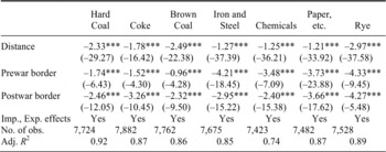
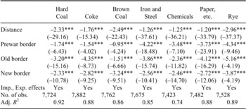
We start by simply the average effects of borders on trade prior to the First World War and after the First World War. We estimate the basic gravity model in levels with time-varying importer and exporter effects as in equation 2 using PPML, trade costs depend on distance, political borders before the war (prewar border), and political borders after the war (postwar border). We do this for the balanced sample and for each product class separately. We always group our data into pre-treatment and post-treatment observations. Table 1 gives the results.

In general, the fit of the model is very good. Distance and the border dummies coefficients are all negative as expected and are highly significant in all cases. As long as the elasticities of substitutions are stable over time for each product class, then the estimated coefficient implies large average effect of national borders on trade between regions before and after the war.Footnote ³⁹ Moreover, the average border effects for various kind of coal are (significantly) larger for the years after the war than before. Instead, the average border effects for iron and steel products, chemical products, and paper are all somewhat smaller after 1919 than before, while those for rye are virtually constant over time.

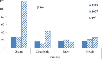
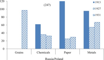
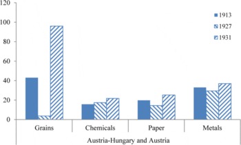
What explains these changes over time? To start with, the interwar period saw a large rise in tariffs and quotas across all products and on nearly all state borders already during the 1920s, but especially after 1929 in reaction to the Great Depression. The best source of comparable tariff data across European states is Heinrich Liepmann who collected data for 1913, 1927, and 1933 for Germany, the Habsburg Empire, and its successor states, the Russian Empire and Poland (after 1918).Footnote ⁴⁰ Figures 1–3 reproduce the relevant data for our sample products: except for trade across the borders of the newly established Polish state tariffs generally increased after the war during the 1920s and then again sharply until 1933.

Moreover, our estimated border effects should reflect not only tariffs along borders but also the impact of quotas and exchange control systems that were imposed on cross-border trade during the Great Depression. All this would suggest an increase in the estimated average border effects after the war. To interpret our results in the light of this intuition note that the estimated border effects γ can be easily converted into tariff-equivalents as exp(γ/-σ^k) −1 (see equation 3). If we take the product group-specific elasticities of substitutions from Caroline Evans, the implied tariff-equivalent of the average “prewar border” on trade in hard coal after the war would be 90 percent, that of the “postwar borders” 150 percent, for iron and steel (semi-) manufactures 291 and 160 percent, for chemicals 137 and 81 percent, for paper and related products 161 and 156 percent, and for rye 155 and 152 percent, respectively.Footnote ⁴¹ Compared to Figures 1–3, these estimates strongly suggest that tariffs are only some part of the story.

FIGURE 1

GERMANY

Notes: Average tariff levels across Central Europe, 1913, 1927, 1933 (unweighted average ad valorem tariffs in percent of product prices based on Liepmann, Tariff Levels)

FIGURE 2

RUSSIAN EMPIRE (1913) AND POLAND

Notes: See the notes for Figure 1.

FIGURE 3

AUSTRIA-HUNGARY (1913) AND AUSTRIA

Notes: See the notes for Figure 1.

The decline in the average border effect after the war that we observe for some goods seems at odds with the increase in tariffs and quotas. But note that these average effects do not reflect the level of trade fragmentation in the sample. First, the number of borders has increased over time. While prior to the war about 7 percent of all trade flows in our sample crossed a national border, it was roughly 10 percent after the war. Therefore, a slight decline in the average border effect, as for example for paper, should not be misinterpreted as evidence for better overall integration.

We can go further if we decompose the postwar borders into “old borders” that existed already before 1914 and “new borders” that were drawn after the war. The lower average border effect that we find in some cases after 1918 might stem from a difference between the effects of “old borders” and those of “new borders.” Were the new borders really excessively trade diverting, i.e., more trade diverting than the old borders, as argued by the losers of the war (parts of whose territories were ceded to neighboring and/or successor states)? Or were instead the peacemakers in Versailles, St. Germain, and Trianon reasonably successful in redrawing the European map such as to minimize additional frictions? In Table 2, we repeat the analysis of border effects but distinguish between the effects of new and old borders after the war (but still without the indicators that tell us when they were put in place).

TABLE 2

AVERAGE BORDER EFFECTS BEFORE AND AFTER WORLD WAR I, OLD AND NEW BORDERS

Note:

The dependent variable is bilateral exports between trade districts. The regression was estimated via PPML on a balanced sample. Standard errors are robust, z-statistics are given in parentheses.

Source:

See the text.

The trade-diverting effect of the new, postwar borders on trade is visible, and it is significant. But the new borders are, on the whole, less nefarious than the older ones, which partly explains why the average border effects declined after the war in some cases. What is more, this finding raises the possibility that borders did not change randomly, but tended to follow some existing structures.

BASIC RESULTS 2: TREATMENT EFFECTS OF BORDERS ARE SMALL

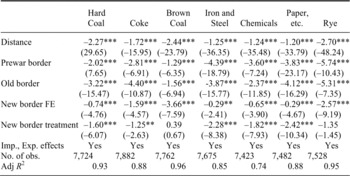
To what extent are the results from Table 2 biased because of unobserved heterogeneity? Obviously, we can explore this question only with regard to those borders that were newly established in 1919/20. To this end we implement the DD estimator in levels, which allows us to distinguish the genuine treatment effect of the news borders (active from 1919 onwards) from a pairwise fixed effect on the treated (FET), active over all periods. Table 3 shows the result.

TABLE 3

TREATMENT EFFECTS OF NEW BORDERS ON TRADE

Note:

The dependent variable is bilateral exports between trade districts. The regression was estimated via PPML on a balanced sample. Standard errors are robust, z-statistics are given in parentheses.

Source:

See the text.

The analysis implies that the border changes followed a pattern of fragmentation that existed before the war: the new border fixed effects (FET) are always negative and highly significant. After controlling for these fixed effects, we find that the treatment effect of new borders is much smaller than the naive cross-sectional estimates in Tables 1 and 2 suggested.Footnote ⁴² If, again, we use the elasticity of substitution from Evans,Footnote ⁴³ the implied tariff-equivalent of the treatment effect of new borders on trade in hard coal is 81 percent (instead of 137 percent as suggested by the cross-sectional estimate from Table 2), for iron and steel (semi-) manufactures it is 109 instead of 129 percent, and zero for rye (or not statistically significantly different from zero, instead of 130 percent). The difference between the two estimates gives the tariff equivalents of time-invariant barriers to trade that run along the new borders. Our results suggest that this is in most cases quite considerable.

To get a more general number on this, we also estimate a pooled version of the PPML-estimator of Table 3, where we pool all data over commodities and allow for the (time-varying) region-effects as well as for the distance-effects to be commodity-specific. These commodity-specific effects capture, for example, differences in prices between commodities, regions, and over time. With this procedure, we find for our total sample of more than 50,000 observations an average treatment effect of the new borders of −0.99 and a new border fixed effect of −1.38 (both highly significant). Taking −3.45 as the average of the commodity-specific elasticities from Evans turns the new border effect into a tariff-equivalent of the treatment effect of 34 percent (compared to 103 percent from naive pooled estimation similar to Table 2).Footnote ⁴⁴ Different assumptions on the elasticity of substitution (for example ranging between −2 and −10) would imply tariff-equivalents (between 64 and 10 percent). But the sign and statistical significance of the effects as well as the relative magnitude of treatment effects as compared to naïve border effects would remain unchanged; in any case the treatment effect would be about 1/3 (0.32 or respectively 0.26 and 0.36) of the naïvely estimated effect that does not control for FET.Footnote ⁴⁵

ROBUSTNESS CHECKS: ADJACENT REGIONS, COUNTERFACTUAL BORDERS, AND, THE GREAT DEPRESSION

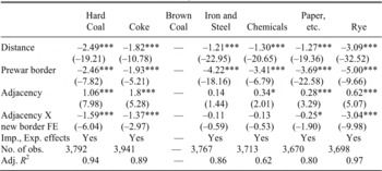
The results of our analysis so far point to political borders having changed broadly along the lines of already existing trade frictions. For this interpretation to hold, trade frictions before 1914 between those pairs of regions that after 1918 were not separated by a new border, should be negligible or at least much smaller than frictions between regions that afterwards were separated by a border. Our model in Table 3 estimated the trade frictions between all pairs of regions that were later separated by a new border using all other pairs of regions as control group. But we can put the idea of a “border before the border” to a harder test. The gravity literature most often finds that neighboring or “adjacent” regions trade significantly more with each other than average trading partners. Let us explore, whether this adjacency effect was present before 1914 for all neighboring regions. If instead, we find prior to 1914 a difference in trade volumes between those adjacent regions that would become separated by a new border after 1918 and the others would remain together, then, the preexisting trade frictions must have been rather strong. Table 4 limits attention to trade flows prior to the war (1885, 1910, and 1913 only). As expected, we find that trade between adjacent regions is significantly above the sample average. However, those adjacent regions that after 1918 were to be separated by a new border were different: here trade flows prior to 1914 were significantly smaller in rye, hard coal, coke, and paper.Footnote ⁴⁶ Note that these are exactly the products for which we find the largest new border fixed effects (see Table 3). In the other two cases (iron and steel products and chemical products), there were generally no significant adjacency effects, nor differences in adjacency effects along future borders.

TABLE 4

“BORDER BEFORE A BORDER?” DIFFERENCES IN TRADE BETWEEN ADJACENT REGIONS, 1885–1913

Note:

The dependent variable is bilateral exports between trade districts. The regression was estimated via PPML on a balanced sample. Standard errors are robust, z-statistics are given in parentheses.

Source:

See the text.

Another way to test our hypothesis is to test for “counterfactual borders.” To this end, we first introduce a dummy for a “counterfactual border” that divides the 43 regions of our sample roughly into a northern and a southern half.Footnote ⁴⁷ Do we find an effect for such a “border” as well? In this case, we find no systematic trade frictions evident along such an imaginary line, neither before nor after the war. This result holds regardless of whether or not we control for the actual borders.Footnote ⁴⁸

We also considered changes that were discussed at the Paris Peace Conference but were not actually implemented. In most cases though, our data is too highly aggregated to consider these as they affect only small territories. The only counterfactual reflected in discussions at Paris that our data allow us to consider is the plan for a “Danubian Federation.” The proposal to replace the crumbling Habsburg Empire with a federation that would allow for regional political autonomy and national “self-determination” without major changes in its internal and external borders received extensive discussion.Footnote ⁴⁹ After the war, the former members of the Habsburg Empire made several diplomatic attempts to halt their disintegration.Footnote ⁵⁰ Given that a “Danubian Federation” would have involved fewer borders rather than additional ones, the counterfactual is not entirely straightforward; not at least because data limitations required us to aggregate Cisleithania. We reestimated the model from Table 3, hence controlling for all factual changes in borders after 1918 but adding dummies for those pairs of regions that would have become part of the “Danubian Federation” (Austria with Czechoslovakia and Hungary, Slavonia, Croatia, and Bosnia).Footnote ⁵¹ Were these regions prior to 1914 well-integrated so that the new borders disrupted their trade network? If so, we would should find positive “new border fixed effects” for the years 1885–1913 and rather strong negative “treatment effects.” In general, we do not.Footnote ⁵² For brown coal, hard coal, coke, and rye, we find (significant) strongly negative new border fixed effects and negative but weak treatment effects in line with all our previous findings. For the remaining commodities estimates did either not converge (chemicals) or they were altogether insignificant. We interpret this as evidence that the “Danubian Federation” did not materialize in part because its economic underpinnings were poor: trade among these regions prior to 1914 was actually limited.Footnote ⁵³

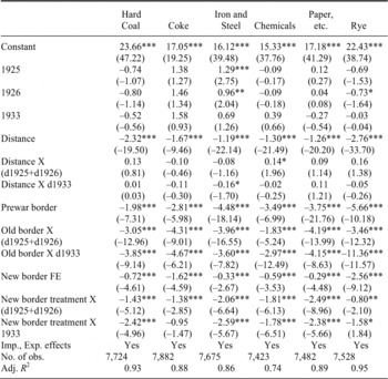
Finally, let us explore to what extent the effect of the new borders on trade changed over time, especially with the Great Depression. While the new borders may have had little effect of trade in the short run because they largely followed existing lines of fragmentation, they nevertheless made new tariffs, quotas, and/or exchange controls possible. Given the sizeable literature on the increase in tariffs and other trade costs in the wake of the Great Depression, one would expect that the new borders became much more detrimental to trade after 1929. To test for this, we change the specification underlying Table 3 in two ways: first we split the constant in a constant for 1885–1913 and year-specific constants for 1925, 1926, and 1933. While this leaves the estimated border effects unchanged, it allows us to visualize the changes in the average level of trade costs that so far have been controlled for by the time-varying importer and exporter effects. Second, we interact the distance variable and the border dummies with year effects for the postwar period. Table 5 gives the results.

To begin, changes in the constant and the effect of distance on trade flows suggests that trade frictions increased between 1926 and 1933. In addition, we also find an increased treatment effect of borders in 1933. However, the increase in trade costs was often larger along the old borders than along the new ones (consider for example the trade costs for rye, but also for chemical products). The new borders did provide a setting for additional trade costs during the Depression, but their impact was small. The new borders did not improve economic integration across Central Europe, but given that border changes were hardly avoidable in 1918, the way these borders were drawn made economic sense—intentionally or not: they imposed only modest additional trade costs.

WHAT EXPLAINS THE “BORDER BEFORE A BORDER”?

The key result of this article is that the new borders after 1918 were less detrimental to trade than earlier research had suggested. This was so because they were, in the main, placed along commercial fault lines that existed already before the war. In the historical literature, the new borders were largely the outcome of protracted bargaining over ethnic or historical claims to territory, strategic concerns, or naked nationalist ambition, with economic reasoning receiving little serious attention at the Paris Peace Conferences. We argue that whatever the motivations of the peacemakers, the outcome of their deliberations on the postwar borders made broadly economic sense.

However, this raises the question which factors account for the “border before a border” effect within the empires of Germany, Austria-Hungary, and Russia, 1885–1913. The most obvious candidates are ethnolinguistic networks and geography. First, consider the prime suspect that also features in the historical literature on the Paris peace settlement: formal or informal institutions that developed along ethnic lines. Ethnolinguistic networks may have mattered because they typically affect trade costs in two ways: they lower them within the network and increase them between network members and those outside. This line of reasoning is supported by recent qualitative work on intrastate economic nationalism and the formation of ethnically based networks within the multinational setting of East Central Europe. Whether boycott movements,Footnote ⁵⁴ “self-integration” of national communities,Footnote ⁵⁵ or the formation of ethnically orientated cooperatives,Footnote ⁵⁶ the evidence points to growing, institutionally organized ethnolinguistic separation in late-nineteenth-century East Central Europe. Thus trade across ethnic group boundaries (as distinct from state borders) likely carried significant costs before 1914. In earlier work on the Habsburg Empire, we found that the effect of ethnolinguistic networks on grain markets starts to be visible around 1883/84, increases up to the mid-1890s, before it stabilizes at a level similar to that in the mid-1880s until the First World War.Footnote ⁵⁷

TABLE 5

TREATMENT EFFECTS BEFORE AND DURING THE GREAT DEPRESSION

Note:

The dependent variable is bilateral exports between trade districts. The regression was estimated via PPML on a balanced sample. Standard errors are robust, z-statistics are given in parentheses.

Source:

See the text.

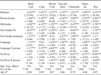
To what extent did ethnolinguistic institutions indeed create barriers to regional trade flows, visible before the actual creation of borders along their lines? Can they account for the observed borders-before-the-border (as visible in the FET)? And did this effect change between 1885 and 1910? To explore these questions, we collected language statistics, which are available for all our regions in 1910. Denote by a_i^k the share of people that declare in the statistic language k as their mother tongue in region i. Similar to a Herfindahl index, we can then construct an index of pairwise ethnolinguistic heterogeneity.Footnote ⁵⁸

(8)

The index takes on values between 0 and 1. An index value of 0 would reflect a pair of regions that has identical shares in each language group; an index value close to 1 would reflect a pair of regions with no overlap in languages spoken. If indeed ethnolinguistic institutions created barriers to regional trade already prior to 1914, such an index should help capture them.

In addition, we can attempt to capture the effects of natural geography that might have separated regions prior to the change in state borders. A simple approach is to distinguish between regions that were connected by navigable rivers (or canals) and those that were not. The first will typically have been better connected already prior to the age of railways, and we can exclude that they were separated by very rugged territory or mountain ranges, while some of the latter may have been. We implement this idea with an indicator variable “No-River” equal to one whenever a pair of regions is not connected by a river or canal. This is arguably a rough approximation to the complex effects of natural geography on trade, but it should give us an indication whether geography matters for the “border before a border” or not.Footnote ⁵⁹ In both cases, ethnolinguistic heterogeneity and natural geography, we distinguish between their effect before and after the war.

TABLE 6

ENDOGENOUS BORDER CHANGES–ETHNOLINGUISTIC HETEROGENEITY AND BORDERS

Note:

The dependent variable is bilateral exports between trade districts. The regression was estimated via PPML on a balanced sample. Standard errors are robust, z-statistics are given in parentheses.

Source:

See the text.

We show the results of this exercise in Table 6. There is indeed evidence that ethnolinguistic institutions had some trade diverting effect both before and after 1919, with a lot of variation across product classes. Except for chemical products, ethnolinguistic heterogeneity reduced trade flows (either only prior to the war as for hard coal and coke or throughout) and in most cases that effect is quite large. In addition, geography as captured by the indicator variable, “No-River” mattered. In all cases except hard coal, regions that were not connected by navigable rivers traded less on railways. Together with the variable on ethnolinguistic heterogeneity, this helps explain a considerable part of the new border fixed effect (FET) that we estimated above. In all cases except for chemical products, the FET coefficients fall, hence we can explain a large part of this effect by ethnolinguistic heterogeneity and natural geography. In some cases (iron and steel products and paper and related products), language and geography eliminate any effect of the new borders.Footnote ⁶⁰ To summarize, regions pairs that were more linguistically different and that were separated by geographic obstacles traded less with each other. Intentionally or not, the peace conferences in effect accounted for this, which explains why we find less of a treatment effect of the new borders than the conventional literature suggests.