The American effort in WWI was partly funded by a series of massive loan drives, in which so-called liberty bonds were marketed to individuals and institutions. Ordinary citizens subscribed to the liberty loans at extraordinary rates, and by 1919, around two-thirds of middle-income households owned a liberty bond.Footnote 1 This transformation of Americans’ finances likely had far-reaching consequences, not all of which were anticipated by the architects of the loan drives. The liberty bond campaigns induced millions of households not only to become the owners of financial assets, but to become the owners of financial assets whose values could fluctuate in response to changes in interest rates. Beginning in late 1919, in an effort to restrain the growth of credit and prices, the Federal Reserve enacted a series of significant increases in its discount rates. This caused the prices of liberty bonds to fall, and millions of American households suffered capital losses. Then, in 1921, the Fed began to ease rates, causing liberty bonds to appreciate again.
We study the electoral consequences of the liberty bond drives and the Fed’s policy changes. The 1920s were a period of Republican dominance in presidential politics, with Harding, Coolidge, and Hoover winning substantial majorities of the popular and electoral votes in 1920, 1924, and 1928, respectively. Previous scholarship has attributed these victories to the breakdown of the coalition that had supported Wilson (Bagby Reference Bagby1962; Burner Reference Burner1968; Murray Reference Murray1976). We posit that voters responded to changes in liberty bond prices by voting against the incumbent Democrats when the bonds depreciated in value and later voting for the incumbent Republicans following the bonds’ appreciation, in a pattern consistent with models of retrospective voting behavior. Such models (e.g., Achen and Bartels Reference Achen and Bartels2016; Healy, Persson, and Snowberg Reference Healy, Persson and Snowberg2017; Hibbs Reference Hibbs2000; Key Reference Key1966; Kramer Reference Kramer1971) argue that voters’ choices are driven by backward-looking assessments of how well the government has performed during an incumbent’s tenure.
Using new data on liberty bond subscription rates, we test whether owning liberty bonds led to changes in voting outcomes in presidential elections in the 1920s relative to those in the previous decade, in a panel of about 1,400 counties. The results indicate that counties with higher liberty bond participation rates turned against the Democrats, relative to their voting patterns in earlier elections. The liberty loan campaigns were guided by the ideal of increasing support for the war and sharing the burdens of war finance equitably (Sutch Reference Sutch2015), but their unintended consequences contributed to an electoral backlash against the party that created them.
Our estimation framework includes county- and state-year fixed effects, which control for any time-invariant county characteristics, such as a historical propensity to vote for a particular party, as well as trends in states’ political preferences. Yet liberty bond subscriptions may have been influenced by unobservable county attributes not reflected in historical voting patterns, which nonetheless influenced voting behavior in the 1920s. To address this possibility, we instrument for liberty bond participation using county-level measures of the severity of the fall 1918 influenza epidemic.
The most lethal wave of the epidemic, which occurred in October 1918, coincided with the largest of all of the liberty bond drives, the campaign for the fourth loan. Our measure of the predicted severity of the influenza epidemic is based on a county’s distance to military training camps, which were an important source of the epidemic within the civilian population. Greater distance from military camps was strongly correlated with participation in the fourth loan, as the bond drive was hampered by both the influenza epidemic itself and by efforts to control the spread of the epidemic. Our instrumental variables estimates of the effect of liberty bond ownership on the Democratic Party vote share indicate that a one-standard-deviation increase in a county’s liberty bond participation rate led to a decrease in the Democratic share in presidential elections of 3.3 percentage points, on average, over the 1920–1932 period.
To assess whether the electoral effects of liberty bonds could have been decisive, we estimate the same empirical model using state-level data. We focus on the 1920 presidential election, in which Democrat James Cox won only 12 states and Harding won 37, for electoral vote totals of 127 to 404. Counterfactual estimates of the Democratic Party vote share for the 1920 presidential election by state indicate that, in the absence of the liberty bonds, the Democratic Party would have won 12 additional states but would still have lost the electoral vote. That is, the effect our analysis attributes to liberty bonds contributed significantly to Republican electoral margins but was unlikely to have been decisive.
This paper contributes to a growing literature on the significance of the liberty bond campaigns in American economic history (Garbade 2012; Tooze Reference Tooze2014; Sutch Reference Sutch2015; Kang and Rockoff Reference Kang and Rockoff2015; Hilt and Rahn Reference Hilt and Rahn2016). Closely related is Julia Ott’s When Wall Street Met Main Street (Reference Ott2011, p. 54), which analyzes the political significance of the liberty bond campaigns, arguing that they “propagate[d] an investor theory of political economy.” Yet Ott’s book mostly neglects the prices of liberty bonds, which are critical for understanding their political consequences. We argue that the most important political legacy of the liberty loan campaigns, which the literature has mostly overlooked, is that they created a large popular class of securities holders who suffered a significant depreciation in the value of their investments under a Democratic president and then experienced a significant appreciation in the value of their investments under the Republicans.
Our analysis also contributes to a much larger literature on the relationship between the composition of households’ wealth and their political beliefs and voting behavior (Guiso et al. 2003; Schreiner and Sherraden Reference Schreiner and Sherraden2006; Ansell 2014; Lewis-Beck, Nadeau, and Foucault Reference Lewis-Beck, Nadeau and Foucault2013; Rahn and Dancy Reference Rahn and Dancy2009). Some of these works have argued that the broadening of stock ownership in the late twentieth century led to increases in the Republican vote share (Cotton and Davis Reference Cotton Nesler and Davis2012; Duca and Saving Reference Duca and Saving2008; Lewis-Beck and Nadeau Reference Lewis-Beck and Nadeau2011; Rahn and Dancy Reference Rahn and Dancy2009), although the literature generally cannot convincingly address the problem that financial asset ownership may itself be influenced by party identification (Huberty 2011).Footnote 2
We advance this literature by studying a historical context with plausibly exogenous variation in financial asset ownership and also by incorporating the performance of financial assets into the analysis. An additional advantage of our setting is its focus on bond values. The depreciations and appreciations in the prices of liberty bonds that occurred between 1919 and 1924 were widely understood to be related to choices made by the Fed and the Treasury. The direct connection between economic policy and bond prices likely strengthens our test of pocketbook concerns in retrospective voting.
FINANCING WWI
Bond Finance
The American effort in WWI led to a nearly 25-fold increase in government expenditures, and funding these expenditures presented an unprecedented challenge. Treasury Secretary McAdoo eventually settled on a plan for a one-third/two-thirds division between taxes and borrowing; tax revenues ultimately accounted for about one fourth of the total (Kang and Rockoff Reference Kang and Rockoff2015; Garbade 2012; Sutch Reference Sutch2015). In addition to helping to maintain lower tax rates, McAdoo believed that borrowing offered another advantage: The ownership of government bonds would give the public a stake in the war effort. In his view, Americans at home would welcome a chance to join the effort in the “financial trenches,” and those efforts would increase support for the war (McAdoo Reference McAdoo1931, p. 378).
Policymakers were keen to make liberty bonds attractive to ordinary Americans and marketed them quite broadly. The bonds were sold in denominations as low as $50, and subscriptions could be fulfilled through installment plans, which made the bonds accessible to a wide range of American households. A $50 liberty bond could be purchased by an initial payment of $4 and then 23 weekly payments of $2. In addition, Treasury allotments were weighted toward smaller investors (Garbade 2012; Sutch Reference Sutch2015). As a result, for the first time, tens of millions of Americans became owners of financial assets other than bank accounts.
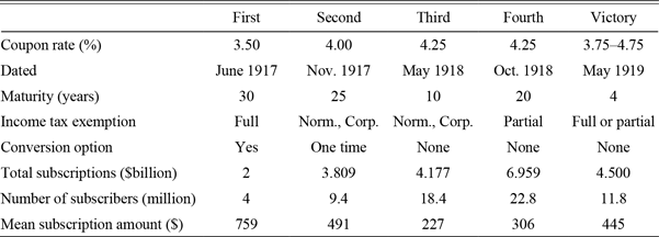
Rather than continuously selling bonds as needed, the liberty loans were marketed through a series of four discrete campaigns, each with a specific sales target; an additional victory loan campaign was conducted following the end of the war. Table 1 presents data on each loan. The bonds were all sold to investors at par, meaning that their initial yield to maturity was equal to their coupon rates. As growing levels of government borrowing put pressure on credit markets, the later bonds were issued with higher coupon rates. In total, the liberty and victory loans raised around $24 billion, equivalent to more than $5 trillion today as a constant share of GDP. The fourth loan alone raised about $7 billion, with nearly 23 million of the nation’s 106 million residents subscribing.
LIBERTY LOAN CHARACTERISTICS AND SUBSCRIPTIONS, BY LOAN

Notes: The first and second loans could be converted into subsequent loans bearing higher coupon rates. Their initial rates are reported here. In addition, some of the victory loan bonds were issued at a lower coupon rate.
Sources: U.S. Treasury (1918–1921); Garbade (2012).
The Liberty Loan Drives
The organization and conduct of the liberty loan campaigns has been described in detail elsewhere.Footnote 3 Briefly, the Treasury Department directed the Federal Reserve Banks to manage bond sales within their geographic districts. They did so by creating state liberty loan committees that, in turn, selected local notables to run county- and city-level organizations. Virtually all of civil society was enlisted by these committees, and organizations as diverse as women’s clubs, the Boy Scouts, and fraternal and religious organizations all contributed to the effort. Local committees recruited a salesforce from these associations, forging “patriotic partnerships” (Skocpol et al. Reference Skocpol, Munson, Karch, Camp and Katznelson2002) to market the bonds as broadly as possible. Over two million people volunteered to participate in selling the bonds (U.S. Treasury 1919). Shoe leather was augmented by extensive advertising and promotion in newspapers, magazines, movie theaters, and department stores. The nation’s economic institutions did their part too. Employers released their workers for liberty loan events, larger companies offered payroll deductions to employees as a way to pay for liberty bond subscriptions, and the nation’s commercial banks advertised the loans to their customers, processed their subscriptions, and offered them safety deposits boxes free of charge for their liberty bond certificates.
Some perspective on the extent to which ordinary households were induced to purchase the bonds can be found in one of the first-ever surveys of American households’ incomes and expenditures, collected by the BLS in 1918/19. The BLS surveyed nearly 13,000 families from the middle of the earnings distribution, who resided in 99 cities (Olney Reference Olney1995; Feigenbaum Reference Feigenbaum2016). Among the surveyed households, nearly 68 percent had purchased a liberty bond in the previous year. This is considerably higher than the rate at which households near the median of the income distribution today own shares of corporate stock, the most widely held risky financial asset.Footnote 4
Some of the rhetoric of the liberty loan campaigns emphasized the attractiveness of the returns that the securities would offer, and many liberty bond ads called them the “safest securities in the world.”Footnote 5 Yet these were negotiable instruments whose values were subject to market forces, and uninformed investors with no experience with financial assets may not have understood that the prices of the bonds could fall. The Treasury did offer non-negotiable war savings stamps to investors of more modest means; for example, stamps that paid $5 in 1923 were sold for just above $4 in January 1918 and could be redeemed prior to 1923 on a fixed schedule of prices (see Garbade 2012, pp. 66–67). Many investors would likely have been better off purchasing war savings stamps, or some vehicle like them, but the Treasury did not promote them as aggressively.
Evolution of Liberty Bond Prices
The WWI years were a period of high inflation in the United States, due in part to rapid expansion of money and credit (Friedman and Schwartz Reference Friedman and Schwartz1963). Yet, even after the Armistice in November of 1918, money and credit growth continued, as did inflation. National banks had committed to lend to subscribers to the fourth loan and the victory loan at 4.25 percent until late 1919, as part of a “borrow and buy” program that helped sell the issues (Meltzer Reference Meltzer2003, p. 93). The Fed supported this program by offering a discount rate that generally ranged from 4 percent to 4.25 percent, and then Treasury Secretary Carter Glass, who was by nature of his office Chair of the Federal Reserve Board, opposed any rate increase. Inflation continued, and concerns mounted that artificially low interest rates were fueling inflation and speculation and causing a significant drain in gold reserves.Footnote 6
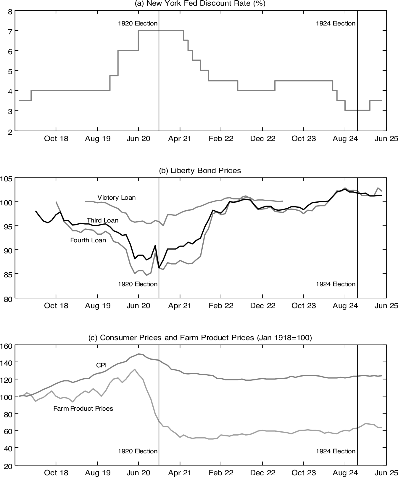
Finally, in December 1919, the Treasury withdrew its objection to rate increases and the Federal Reserve Banks began to raise their discount rates, with the blessing of the Board. Partly as a result of its inexperience with such matters, these rate increases were “not only too late but also probably too much” (Friedman and Schwartz Reference Friedman and Schwartz1963, p. 231). The New York Fed’s discount rate was increased from 4 percent to 4.75 percent in December 1919, then 6 percent in January 1920, and finally 7 percent in June 1920, an extraordinary level that was not reached again until the 1970s. Some of the Reserve Banks began to impose “progressive” or increasing rates on banks that were heavy borrowers at their discount windows as well (Melzer Reference Meltzer2003, p. 106). This induced a rapid contraction in financial markets and in economic activity, triggering a severe recession. The Fed ultimately began to ease its rates in April 1921 in a series of 0.5 percent cuts that brought the discount rate back down to 4 percent by June 1922.
Liberty bond prices were closely connected to these changes in the Fed’s rates. The increases in the Fed’s rates in 1919/20 led to increases in the yields on liberty bonds, which were produced by a fall in prices. In addition, large quantities of the issues that had been purchased through the borrow and buy policies were sold by the original subscribers when the rates on loans collateralized by liberty bonds increased; this selling pressure likely contributed to the fall in prices as well.
Figure 1 shows how this process unfolded. Panel (a) shows the New York Fed’s discount rate, and how it ratcheted up quite steeply in late 1919 and early 1920 and was then lowered beginning in 1921. Panel (b) presents the steep drop in the prices of the loans that resulted, in a pattern that varied inversely with the New York Fed’s discount rate. Beginning in 1921, those prices began to recover and the price increases continued into 1922–1924.
THE FED’S DISCOUNT RATE, LIBERTY BOND PRICES, AND FARM PRODUCT PRICES

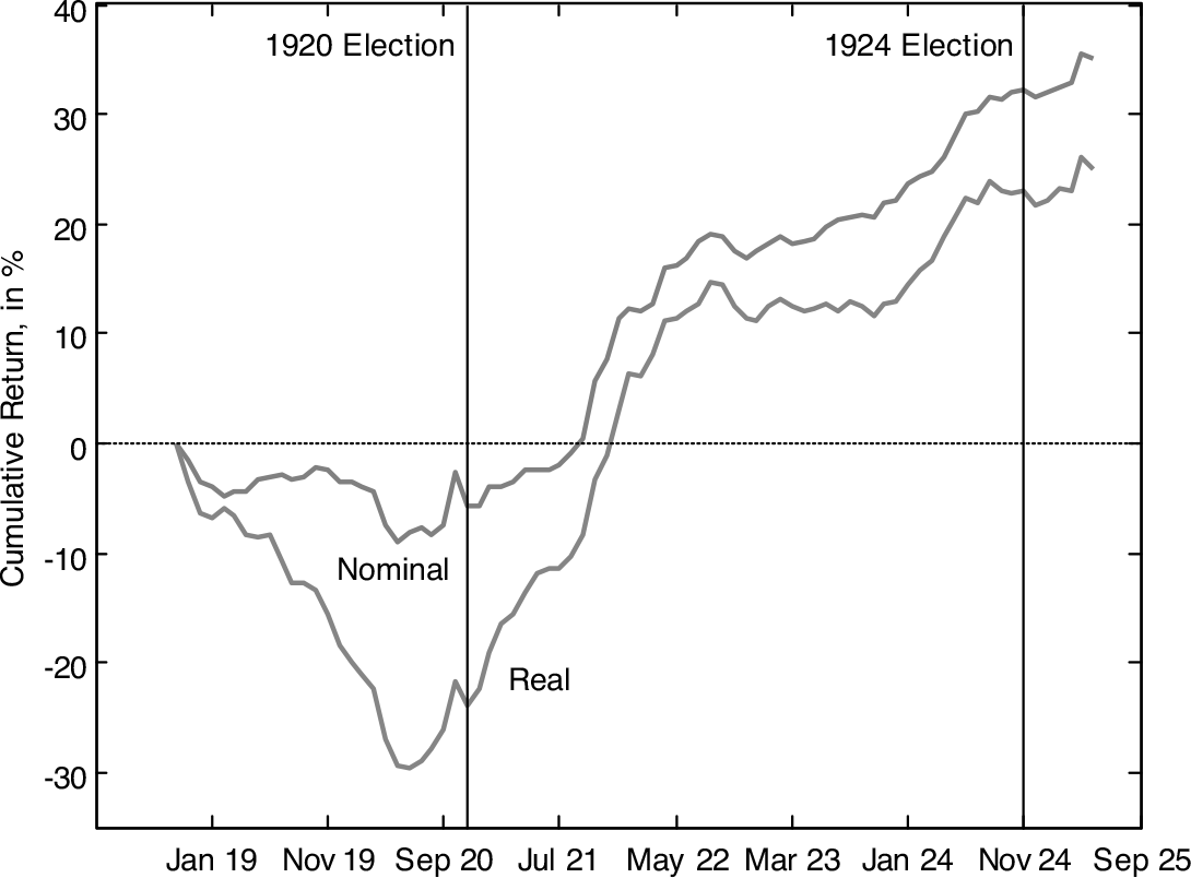
An indication of the effects of these fluctuations for ordinary investors during the presidential campaigns of 1920 and 1924 can be found in Figure 2, which presents the cumulative returns received by subscribers to the fourth loan, in both nominal and real terms. Over the two years between the issuance of the bond and the 1920 election, the depreciation in the prices of the bonds was greater than the coupon income and the total cumulative returns received by holders of the fourth loan were negative: –5.8 percent (see the Online Appendix for details). The subsequent appreciation of the bonds produced very strong returns over 1921 and 1922, and by the time of the 1924 election, cumulative returns had risen to 32.3 percent, slightly better than what a constant 4.25 percent annual return would have produced.
CUMULATIVE RETURNS FOR THE FOURTH LIBERTY LOAN, 1918–1925

Panel (c) of Figure 1 illustrates an additional consequence of the Fed’s tightening: deflation—in particular, a sharp decrease in commodities prices. The Fed’s tightening caused the dollar to appreciate, which caused traded commodities prices in the United States to collapse.Footnote 7 The decline of farm product prices in 1920/21 had devastating effects on rural areas and presents an alternative potential source of discontent regarding incumbents in the 1920 elections that will be addressed below.
POLITICAL IMPACT OF LIBERTY BOND PRICE CHANGES: NARRATIVE EVIDENCE
The fall in liberty bond prices in 1919/20 was widely reported in the financial press and aroused considerable agitation. Given that millions of households had been induced to become bond holders by the federal government, the collapse in bond values was perceived as a betrayal. In one response, Representative Walter Magee, a Republican from New York, introduced HR 501 in April of 1920, calling for the appointment of a special bipartisan committee to investigate the decline in liberty bond prices. In a hearing before the House Rules Committee a month later, Magee inserted in the Congressional Record a variety of written material from around the country accusing the government of reneging on its promise to provide its patriotic citizen investors with the safest investment in the world. The public, the committee was informed by the editors of the Syracuse News, was “disillusioned—distressingly so … It is sore and disgusted and does not disguise the fact.” The editorial went further, averring that the people of the United States “will not care to be singed twice in the same place” should the government need to come calling again (U.S. Congress 1920).
For most liberty bond owners, the capital losses suffered as a result of the price depreciation were probably relatively modest. At its nadir, the market price of a $50 share of the fourth liberty loan was about $42.50, implying a loss of about $7.50. For comparison, the median income of liberty bond owners in the BLS survey was about $1,500. In the context of a deep recession, many households likely suffered far greater losses on the values of their homes, on crop income due to the fall in agricultural commodity prices, or in labor income if they became unemployed or saw their hours reduced. But this is precisely why the depreciation of the bonds provoked such rancor: At a time when the savings embodied in the bonds were needed most, 15 percent of their value was gone. Although these were merely paper losses that would be reversed if the bonds were held to maturity, some subscribers of modest means had to sell their bonds at the bottom of the market “to furnish cash for living expenses” (Evening Star [Washington DC], 16 October 1920.)
The Democratic and Republican parties were less consistently ideological at the time than they are today and represented diverse coalitions of interests that shifted somewhat in the 1920s (Burner Reference Burner1968). Yet it is safe to say that the agenda of the Republicans was generally more friendly to business and finance, and during the 1920 campaign, the Republicans seized the opportunity to criticize the Democrats for the financial mismanagement that they claimed had led to the price declines. The Republican National Committee ran newspaper advertisements in competitive states that pointed out that, after making sacrifices to buy the bonds, subscribers “must make further sacrifices, if compelled to sell those Liberty Bonds, in order to meet the abnormal conditions confronting [them]…”Footnote 8 But perhaps the clearest indication that the welfare of liberty bond subscribers was important to the 1920 election campaign was their prominent appearance in the Republican Party platform, which mentioned the “serious loss” suffered by the millions of liberty bond subscribers.Footnote 9 The Republicans appealed to securities holders who had seen their investments fall in value, and their message of sound financial management likely resonated among a broad segment of the electorate.
Harding won with a substantial popular and electoral majority. Some commentary following the election did suggest that the depreciation of liberty bonds was among the “fundamental causes” of the Democrats’ defeat (“Some Observations on the Causes of the Defeat,” Montgomery Advertiser, 11 November 1920, p. 4.) One prominent newspaper’s editorial board suggested a connection between the enfranchisement of women and the turn against the Democrats: since many women “pinched and saved” to purchase liberty bonds, only to see those investments lose value, “women changed many normal Democratic votes to Harding” (“How the Women Voted,” Philadelphia Inquirer, 5 November 1920, p. 12.)
As the Fed eased interest rates in 1921 and 1922, liberty bonds appreciated in value. Senator Simeon D. Fess of Ohio, in a speech construed to be a semi-official announcement of Harding’s re-election bid, extolled the accomplishments of the president and invited the public to behave just like models of retrospective voting say they ought to: “President Harding has been in office just two years. Those two years have been crowded with a great volume of constructive and remedial work. The record is now made up; the results are apparent upon which the people must give their verdict of approval or disapproval (emphasis added)” (Chicago Daily Tribune, 10 April 1923). The return of liberty bonds to par was specifically mentioned by Fess as an indicator of the prosperity occasioned by the administration’s policies.
Harding did not live to see himself re-nominated. His vice president, Calvin Coolidge, succeeded him and received the Republican nomination for president the next year. Despite Democratic charges of corruption and a whistle-stop campaign featuring a Singing Teapot (Shulman 2015), Coolidge went on to a comfortable win. The Republican Party platform of 1924 began by reminding voters just how bad things were when the party took over: “there were four and half million unemployed; industry and commerce were stagnant; agriculture was prostrate; business was depressed; securities of the government were selling below their par values” (emphasis added). Now, thanks to Republican rule, things were considerably improved: The federal budget deficit had been erased, taxes lowered, and “[g]overnment securities increased in value more than $3,000,000,000.” If holders of liberty bonds behaved as retrospective voters, we would expect them to “Stay Cool with Coolidge” by rewarding his administration with their votes.
DATA
For the purposes of this paper, we assembled a new dataset of county liberty bond subscriptions for several Federal Reserve Districts. In this section, we provide a brief overview of our sources and variable definitions; more detail is provided in the Online Appendix.Footnote 10
Our subscription data were collected from pamphlets published by the Federal Reserve Banks’ liberty loan committees, which presented information on sales of one or more liberty loans. Most of these pamphlets were found at the National Archives, in Princeton University’s Mudd Manuscript Library, or in the Library of Congress. As we are interested in voting outcomes, we use data on subscription rates, defined as the number of subscribers reported for a county divided by the county’s 1920 population. We focus our analysis on the fourth liberty loan, the largest issue, and the one for which we found data for the greatest number of counties. The fourth loan had the highest participation rates of all the loans, and the subscription rate for that loan provides a reliable indicator for the minimum extent to which a county participated in the liberty bond drives.
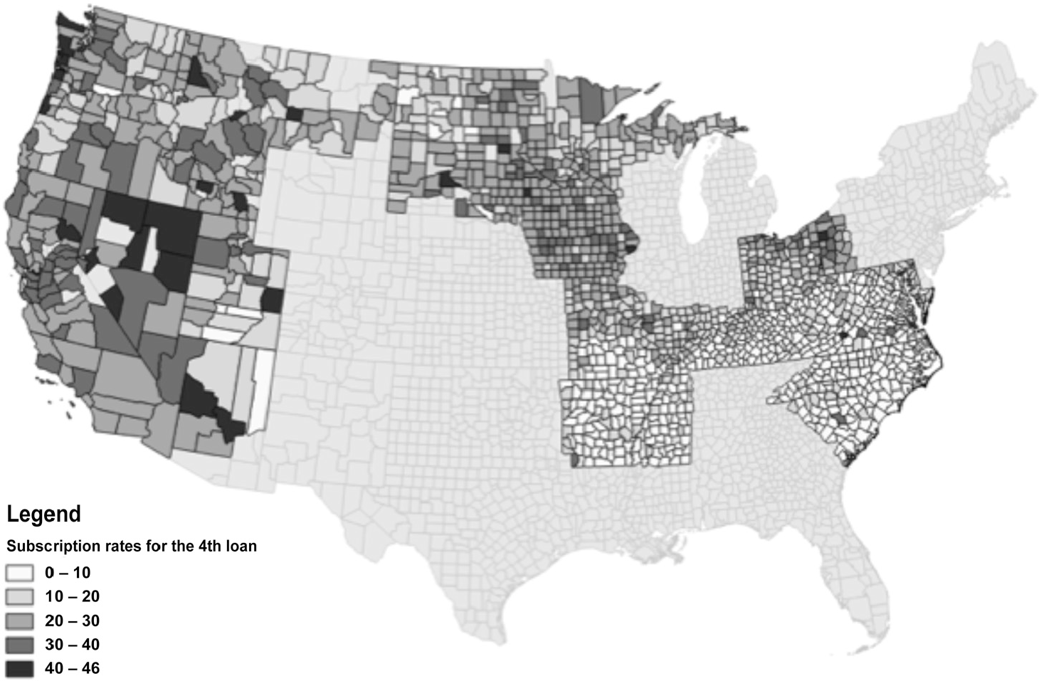
We match these liberty bond subscription rates to data on county voting patterns from a dataset compiled by Clubb, Flanigan, and Zingale (Reference Clubb, Flanigan and Zingale2006). To control for county characteristics, we also match these counties to 1920 county characteristics reported in historical federal censuses, compiled in Haines (Reference Haines2010). Our liberty bond subscription data are illustrated in Figure 3, which presents a map of the counties for which we have data for the fourth loan, shaded by the level of subscriptions. The irregular geographical coverage of the sample reflects the fact that we have data from the Fourth District (Cleveland Fed), Fifth District (Richmond), Eighth District (St. Louis), Ninth District (Minneapolis), and Twelfth District (San Francisco), plus the state of Iowa. The data in the figure present some clear regional patterns: Subscription rates were relatively low south of the Mason–Dixon line and higher in the upper Midwest and West. This presents a challenge for the analysis: Geographical variation in liberty bond participation rates may produce spurious correlations with variables with similar geographic patterns, including voting outcomes. In what follows, we use a variety of approaches to address this challenge.
SUBSCRIPTION RATES, FOURTH LIBERTY LOAN

EMPIRICAL ANALYSIS: LIBERTY BONDS AND ELECTION OUTCOMES
County Panel Estimates
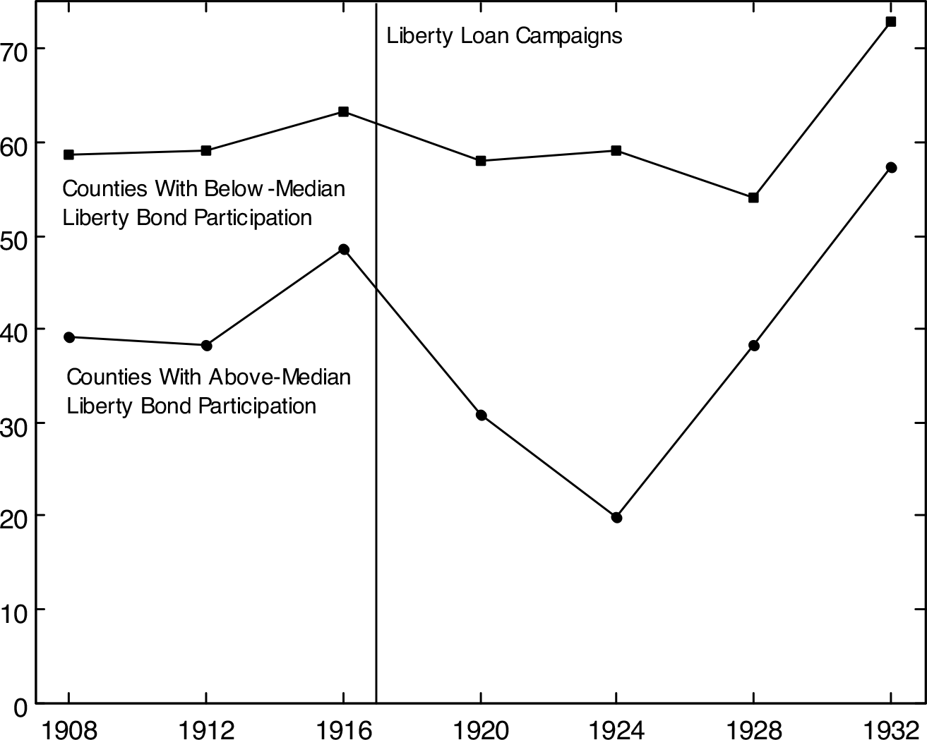
A simple exploration of the effects of the liberty bonds on election outcomes is presented in Figure 4, which compares the Democratic vote shares in presidential elections for counties with above-median levels of participation in the loan drives to those of counties with below-median participation rates. In the 1908–1916 elections, the above-median participation counties voted for the Democrats at rates that were consistently lower than the counties with below-median participation, a likely consequence of the fact that they tended to be located in the North and West, were more urban, and were wealthier. Yet, importantly, the two lines remained parallel up to 1912 and then the Democratic vote share increased differentially for the high-participation counties in 1916. This indicates that there was no ongoing trend toward a differentially declining Democratic vote share among the high-participation counties in the years prior to the liberty loan drives; if anything, the opposite occurred in the 1916 election.
DEMOCRATIC VOTE SHARE: COUNTIES WITH ABOVE- AND BELOW-MEDIAN LIBERTY BOND PARTICIPATION RATES, 1908–1932

The patterns in the figure over the subsequent years suggest a potentially large effect of the liberty loan drives. The high-participation counties turned away from the Democratic Party at high rates in 1920 and 1924, whereas the low-participation counties’ voting behavior remained quite stable. This suggests that the growing difference between the two sets of counties over these years, which will be the focus of the regression analysis that follows, was due to changes in the voting behavior of the counties that actually subscribed to the liberty bonds, and not due to changes among other counties. Then, in 1928, with the large fluctuations in the liberty bonds’ prices a distant memory, the high-participation counties reverted to voting for the Democrats at the same rates as in 1908–1912. Finally, the 1932 electoral landslide, in which the political preferences of both sets of counties took an extraordinary turn toward the Democrats, appears to have had little relationship with liberty bond subscriptions.
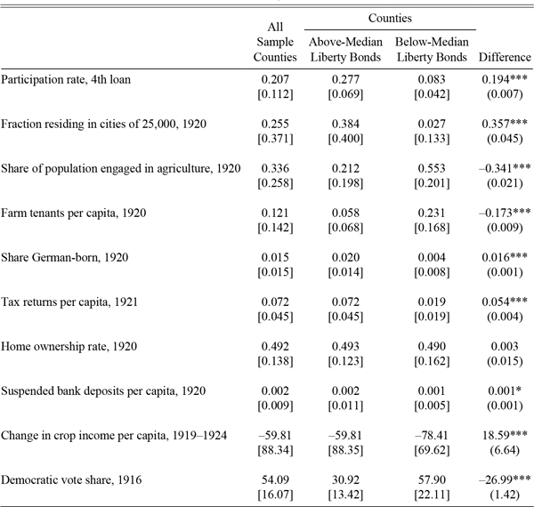
Of course, these two groups of counties differed in many ways beyond their liberty bond subscription rates, and these differences must be accounted for in any empirical tests. Summary statistics for the 1920 values of many county characteristics are presented in Table 2.Footnote 11 The data in the table show that counties with above-median subscription rates were more urban and less agricultural and had fewer farm tenants, more German-born residents, and more households whose income was high enough that they had to file income tax returns as a share of their populations. On the other hand, the home ownership rate was quite similar across the two groups of counties. The recession induced by the Fed’s tightening in 1919/20 created significant financial distress, which was concentrated in agricultural areas (Jaremski and Wheelock Reference Jaremski and Wheelock2019). Consistent with the fact that they were less agricultural, the high-participation counties experienced less of a decrease in crop income from 1919 to 1924. However, those counties actually had a slightly greater level of deposits per capita in suspended banks in 1920. Each of these differences could have influenced political behavior in the 1920s.
SUMMARY STATISTICS, COUNTY DATASET

Notes: All statistics are weighted by 1920 county population. Standard deviations are in brackets; robust standard errors obtained from cross-sectional regressions are in parentheses. *p < 0.1, **p < 0.05, and ***p < 0.01.
Sources: Haines (Reference Haines2010); Clubb, Flanigan, and Zingale (Reference Clubb, Flanigan and Zingale2006); various archival sources. See the Online Appendix.
Our empirical model of the effects of liberty bond participation on election outcomes from 1908 to 1932 takes the following form:
 $$Demshar{e_{ist}} = \;{\alpha _i} + {\gamma _{st}} + \delta libloanpartici{p_i} \times post{18_t}\; + \;\beta {X_{it}} + \;{\varepsilon _{it}},$$
where αi is a county fixed effect, γst is a state-by-year fixed effect, libloanparticipi × post18t is an interaction between the county’s liberty loan participation rate and an indicator for elections in the years following the liberty loan campaign, and Xit includes 1920 county characteristics interacted with post-1918. County fixed effects absorb any unchanging county characteristics (such as location in the South), and state-year fixed effects absorb any trends in the political preferences of particular states over time (such as Kentucky becoming less aligned with the Democrats). Only the variation over time among counties within the same state, which is δ in Equation (1), will be used to estimate the effects of liberty bond subscriptions. The identifying assumption of this framework is that, in the absence of the liberty bonds, the rate at which the high-participation counties would have voted for the Democratic Party in the 1920s would have evolved in parallel with the rate at which low participation counties in the same state did, conditional on Xit.
Presidential politics in the 1920s differed from that of prior decades, as the coalitions supporting each party and the policy questions at the center of partisan debates both shifted (Burner Reference Burner1968). The many economic, social, and demographic differences across counties of varying levels of liberty bond subscriptions could have created differential changes in county voting patterns in the 1920s, violating the identifying assumption of the model. To ensure that any political effects of these county characteristics in the 1920s do not confound our estimates of the impact of liberty bond subscriptions, in Equation (1), we also include 1920 county characteristics interacted with a post-1918 indicator, represented by Xit.
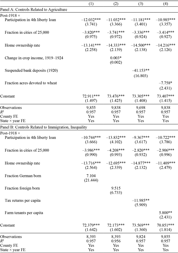
Table 3 presents the results. Column (1) in Panel A presents the estimates from a specification that includes post-1918 interactions with liberty bond participation rates and also 1920 county homeownership rates and the fraction of the population residing in cities of more than 25,000. The estimated effect of liberty bonds implies that a one-standard-deviation increase in participation led to a decrease in the Democratic Party vote share of about 1.3 percentage points (= –12 × 0.11). As the median margin of victory for the Republican Party among the sample counties was 5.6 percentage points, this effect is modest, but not irrelevant.
EFFECT OF LIBERTY LOAN PARTICIPATION ON THE DEMOCRATIC VOTE SHARE, 1908–1932: OLS

Note: This table presents OLS regressions of the effect of liberty loan participation on the Democratic Party vote share in presidential elections, in a panel of counties. All regressions are weighted by 1920 county population. Robust standard errors clustered by county are presented in parentheses. *p < 0.1, **p < 0.05, and ***p < 0.01.
Sources: Authors’ calculations from data in Clubb, Flanigan, and Zingale (Reference Clubb, Flanigan and Zingale2006), Haines (Reference Haines2010), and various archival sources. See the Online Appendix.
In the remaining columns of Panel A, we include variables related to the extent of economic distress in agriculture as additional controls. Consistent with economic dislocations causing voters to turn against the Democrats, the change in crop income from 1919 to 1924 (Column (2)) had a positive effect on the Democratic vote share and the amount of suspended bank deposits per capita in 1920 (Column (3)) had a negative effect. During the war years, wheat prices were partly controlled, whereas cotton prices were not, and wheat farmers resented the Democrats’ preferential treatment of Southern cotton growers (Bagby Reference Bagby1962). Although the collapse of wheat prices beginning in mid-1920 was not as severe as that of cotton prices (see the Online Appendix), wheat farmers may have been especially likely to turn against the Democrats, and the estimate associated with the fraction of acres devoted to wheat (Column (4)) indicates that this was indeed the case. Yet none of these variables substantially changes the estimated magnitude of the effect of liberty bonds on election outcomes in the 1920s.
Many German Americans opposed Wilson’s decision to enter WWI and resented the terms of the Treaty of Versailles, while immigrants from other countries opposed the League of Nations and the Democrats’ anti-immigration agenda (Bagby Reference Bagby1962; Burner Reference Burner1968). For these reasons, immigrants turned against the Democrats in the early 1920s (Tabellini Reference Tabellini2017). As immigrants were singled out by the liberty loan campaigns and purchased the bonds at high rates (Hilt and Rahn Reference Hilt and Rahn2016), their voting patterns in the 1920s, which may not have been driven by the returns to owning liberty bonds, could be responsible for our results. Yet including measures of the fraction German born or foreign born (Columns (1) and (2) in Panel B of Table 3) does not affect the magnitude of the estimated effect of liberty bonds on the Democrats’ vote share.Footnote 12 Finally, in Columns (3) and (4) of Panel B, measures related to wealth and inequality—tax returns per capita and farm tenants per capita—are included. Again, the parameters associated with liberty bonds are not substantially changed.
Women were guaranteed the right to vote by constitutional amendment in 1920. A potential concern regarding our analysis could be that counties with greater political engagement by women, which would have led to higher liberty bond participation, may have turned toward the Republicans in 1920 for reasons unrelated to liberty bond prices. Yet, in the Online Appendix, we show that the effect of liberty bond subscriptions on the Democratic vote share in 1920 was no greater in states where women were enfranchised for the first time in that election, compared to states where women had already been granted the right to vote in 1916.
In Section 3.7 of the Online Appendix, we estimate an alternative version of Equation (1) with separate effects for each election, rather than an averaged post-1918 effect. The only elections where liberty bond participation rates had significant effects were those of 1920 and 1924—the elections that followed the large deprecation and appreciation in the liberty bonds’ values. This helps rule out the possibility that the effects we ascribe to the liberty bonds were the product of ongoing trends that were correlated with liberty bond participation rates.
Next, to rule out the possibility that unobservable county characteristics may be responsible for our results, we use an instrumental variable.
An Instrumental Variable Based on the 1918 Influenza Outbreak
The campaign for the fourth loan, which was conducted between September 28 and October 19, coincided with the deadly 1918 influenza epidemic in the United States.Footnote 13 Efforts to promote the fourth loan were hampered by many individuals’ reluctance to attend public events for fear of exposure to influenza, by sickness and incapacitation among the members of the organizations tasked with promoting bond sales, by lost incomes due to illness and business closures, and by measures imposed to halt the spread of the epidemic, such as prohibitions against public assemblies.Footnote 14 Treasury officials stated that the epidemic created “a great handicap” for the loan campaign.Footnote 15 The goals for the campaign’s total sales were ultimately met, but the subscription rates within the population—the focus of this study—were likely reduced as the campaign organizers leaned more heavily on institutional purchasers to meet their sales goals. If the epidemic reduced subscription rates to varying degrees around the country, and if it had no consequences on election outcomes beyond those resulting from its effects on the loan campaigns, then it would represent the source of a valid instrument.
There is some evidence that the influenza epidemic did not have significant direct electoral consequences, which would imply that the exclusion restriction for the instrument would be met. Achen and Bartels, for example, review the existing literature and present a careful analysis of the 1918 Congressional elections. They conclude that voters “thought of the pandemic as part of the natural world rather than as part of the social world” and did not punish incumbents in places where the outbreak was more severe (Reference Achen and Bartels2004, p. 34).
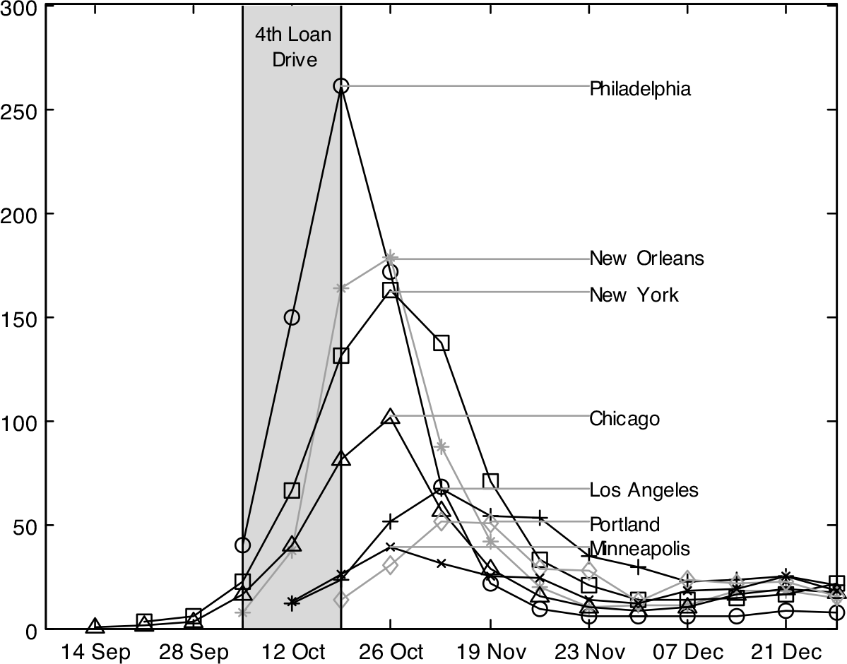
The severity of the outbreak did vary significantly across the country. Influenza deaths per 100,000 residents for seven major cities are plotted in Figure 5. Among the cities in the figure, the outbreak in Philadelphia was the deadliest, with the city enduring more than 600 deaths per day during the week of October 19. By contrast, the outbreak was less severe in Chicago and Minneapolis. In addition, although the outbreak in Portland was deadlier than the outbreak in Minneapolis, it peaked somewhat later and death rates during the fourth loan campaign were lower there. Variation in the severity of the influenza outbreak will serve as our main instrumental variable; we also use a measure of its timing in the construction of an alternative instrument, which we present in the Online Appendix.
WEEKLY DEATHS PER 100,000 RESIDENTS FROM INFLUENZA AND PNEUMONIA, 14 SEPTEMBER–28 DECEMBER 1918

Unfortunately, weekly data on influenza deaths are available for only a small number of cities and monthly deaths from all causes are available for only 530 cities located in 369 counties.Footnote 16 To construct a measure of the severity of the influenza outbreak, we use each county’s proximity to the source of the epidemic within the United States: military camps. During the war, draftees were sent mainly to 32 large camps to receive training and sometimes later sent to a handful of additional camps to prepare for deployment overseas. These camps were often quite overcrowded, and as they were populated by young men—those at an age that made them unusually vulnerable to the 1918 influenza—they constituted an environment especially conducive to the spread of the epidemic. In fact, the epidemic was so acute within the military that total deaths due to influenza among military personnel were similar in number to combat deaths (Byerly Reference Byerly2010). Although the camps were put under quarantine when large numbers of soldiers fell ill, these quarantines were often enacted too late and enforced imperfectly, making the armed forces “the foci from which the civilian population received the disease” (Crosby Reference Crosby2003, p. 56; Byerly Reference Byerly2005, p. 79).
The locations of the military’s camps are shown in Figure 6A. Scholarship on the pandemic has associated proximity to the camps with the severity of influenza in 1918. Crosby (Reference Crosby2003, p. 71), for example, suggests that Philadelphia’s location near both Camp Dix and Camp Meade contributed to the outbreak in that city; Camp Mills and Camp Humphreys were just slightly farther away. The irregular distribution of the camps suggests that the distance to the nearest camp was unlikely to fully capture a county’s exposure to the disease from the military. Some counties were located a relatively short distance from a single military base, whereas others—such as those in central Missouri or southern Illinois—were located a similar distance from several. As the wartime movements of troops spread influenza not only among the camps, but also into the civilian populations along the routes followed by railroads that connected the camps’ locations, counties located near more than one camp were particularly likely to be exposed to the pandemic from the military. We, therefore, use the average distance from a county to each of the camps as our measure of predicted influenza severity.Footnote 17 These distances for our sample counties are illustrated in Figure 6B.
LOCATION OF WWI MILITARY CAMPS

AVERAGE DISTANCE TO MILITARY CAMPS AMONG SAMPLE COUNTIES

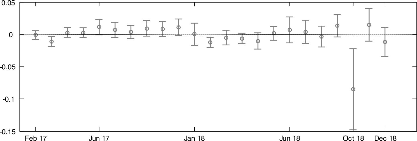
To verify that these distances were correlated with the severity of the influenza outbreak, we investigate their relationship with mortality within the 369 counties for which deaths from all causes can be observed. To verify that any October 1918 mortality effect does not simply reflect something present in all months, the relationship between distance to the camps and mortality is estimated for every month in 1917 and 1918, in a framework with county fixed effects. The estimates, presented in Figure 7, show that distance to the camps was an important determinant of county mortality in October 1918, but not in other months. The negative effect on mortality in October 1918 has a large standard error but is, nonetheless, consistent with a substantial mortality advantage during the fall influenza outbreak.Footnote 18
ESTIMATED EFFECT OF DISTANCE TO MILITARY CAMPS ON MORTALITY: 369 COUNTIES, JANUARY 1917–DECEMBER 1918

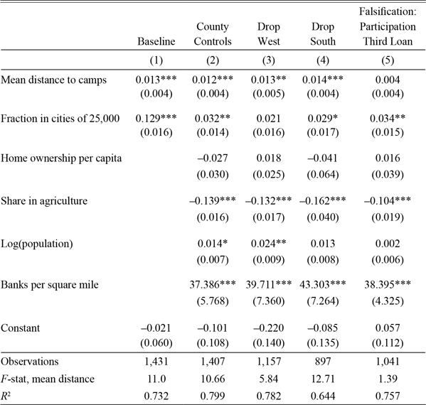
The validity of the distance measure as an instrument for participation in the fourth loan is explored in Table 4. The table presents cross-sectional regressions of the relationship between distance to camps and participation in the fourth loan for the counties for which we have liberty bond data. (These are cross-sectional versions of the first stage from the panel regressions presented below.) The results in Columns (1) and (2) indicate that distance to military camps had a robust positive effect on liberty bond participation, consistent with greater distances resulting in a less severe outbreak of influenza, and therefore fewer influenza-related problems in the conduct of the bond drive. In Columns (3) and (4), the counties of the West and South are dropped and the point estimate associated with mean distance remains generally unchanged.
“FIRST STAGE” REGRESSIONS OF THE RELATIONSHIP BETWEEN DISTANCE TO CAMPS AND PARTICIPATION IN THE FOURTH LOAN

Note: This table presents cross-sectional regressions of the determinants of county-level participation in the fourth liberty loan. (This is the cross-sectional analog of the first-stage regressions in the panel specifications presented below.) All regressions are weighted by 1920 population. Robust standard errors clustered by state are presented in parentheses. *p < 0.1, **p < 0.05, and ***p < 0.01.
Sources: Authors’ calculations from data in Haines (Reference Haines2010), U.S. War Department (1920), and various archival sources. See the Online Appendix.
The mechanism behind the distance measure we propose operates through the influenza outbreak and not through other institutional or economic characteristics that may also have been correlated with distance to the camps. To address the latter possibility, Column (5) presents a falsification test: The participation rates for the third liberty loan, which was conducted in April 1918—before the lethal influenza outbreak in the fall—are regressed on the distance measure. If distance to the camps was correlated with higher participation in the fourth loan because it was correlated with particular social or economic characteristics that led to higher subscriptions, then it should also have been correlated with higher participation in the third loan. Yet the estimate in Column (5) indicates that its effect on the third loan was far smaller.
Additional evidence in support of the hypothesized relationship between distance from the camps, influenza, and the fourth loan campaign can be found in an official account of the progress of the drive for the fourth loan printed in newspapers on 18 October, including the New York Times. Footnote 19 The statement included one-sentence accounts of the state of the campaign in each district, some of which mentioned problems related to influenza, whereas others did not. For example, the statement from the Federal Reserve Bank of Philadelphia was “making a real battle against enormous odds caused chiefly by influenza,” whereas that of San Francisco said simply “maintaining steady increase in face of bad agricultural conditions in some sections.” Comparing the average distance to military camps among the counties in districts where influenza was and was not mentioned as an important hindrance to the loan drive reveals that the districts where influenza was not mentioned were indeed located farther away from the military camps, by about 215 km.Footnote 20
IV Estimation
We now turn to the estimation of our model with instrumental variables. The equation to be estimated is the same as Equation (1), only libloanparticipi} × post18t will be instrumented with distancetocampsi × post18t. As with our ordinary least squares (OLS) estimation, we include county and state-by-year fixed effects, which means that only the variation within states in distances to military camps and loan participation rates will be used to identify the effects of liberty bonds. The exclusion restriction for the instrument requires that distances to military bases among the counties within each state were uncorrelated with any county characteristics other than liberty bond subscriptions that may have shifted political preferences in the 1920s.
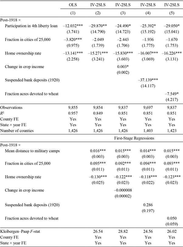
The results are presented in Table 5. Column (1) presents the OLS estimate, and Column (2) presents the same specification estimated with two-stage least squares (2SLS). The main parameter of interest, the effect of liberty bond participation on the Democratic Party vote share, is larger with 2SLS. The greater magnitude of the estimate may reflect the subset of the population from which the parameter is identified: persons who were induced to purchase liberty bonds, or not to purchase liberty bonds, purely as a result of the local severity of the influenza epidemic, and therefore the conduct of the liberty loan campaign. These are likely to have been investors who were less committed to purchasing liberty bonds, either due to financial resources or ideology, and may have been more likely to regard the fluctuations in the bonds’ prices as a betrayal. On the other hand, the standard error of the 2SLS estimate is also quite large; in fact, the difference between the 2SLS and OLS estimates is not statistically significant.Footnote 21
EFFECT OF LIBERTY LOAN PARTICIPATION ON ELECTORAL OUTCOMES, 1908–1932: 2SLS RESULTS

Notes: This table presents OLS and 2SLS regressions of the effect of liberty loan participation on the Democratic Party vote share in presidential elections, in a panel of counties. The instrument for liberty loan participation is the mean distance of a county to military camps, a determinant of the severity of the 1918 influenza epidemic. All regressions are weighted by 1920 county population. Robust standard errors clustered by county are presented in parentheses. *p < 0.1, **p < 0.05, and ***p < 0.01.
Sources: Authors’ calculations from data in Clubb, Flanigan, and Zingale (Reference Clubb, Flanigan and Zingale2006), Haines (Reference Haines2010), U.S. War Department (1920), and various archival sources. See the Online Appendix.
Columns (3)–(5) add some of the same controls as in Table 4; the first stage of each equation is presented in the lower panel. Particularly important is the regression in Column (5), where we control for the fraction of the county’s agricultural acreage devoted to wheat. As noted above, wheat farmers may have been particularly resentful against the Democrats, and the average distance to military camps was often quite high in the wheat-growing regions of the upper West.Footnote 22 The positive correlation between the instrument and this marker for differential hostility to the Democratic Party, therefore, could explain our IV results. Yet controlling for wheat acreage does not change our main estimates.
Our preferred specification is that of Column (2). The estimated effect of liberty bonds implies that a one-standard-deviation increase in subscription rates led to a 3.3 percentage point (= –29.9 × 0.11) decline in the Democratic Party’s vote share in the elections of the 1920s. Another way to judge the size of this effect is to note that it implies that the Democratic Party’s vote share fell by a population-weighted 6.1 percentage points, on average, across all sample counties, due to the effects of liberty bonds.
A natural concern about these results relates to the exclusion restriction for the instrument. One can certainly imagine channels through which proximity to military bases may have influenced electoral outcomes. For example, proximity to military camps could have fueled patriotism or nationalism, potentially leading to stronger support for Republicans. Alternatively, many of the camps were closed at the end of the war, and one might imagine that the decline in economic activity from the demobilization in the areas surrounding the camps may have led to discontent with incumbent politicians. Yet the reduced-form version of the IV model (presented in the Online Appendix) shows that the effect was exactly the opposite: The closer a county was to military camps, the less likely it was to turn against the Democrats in the 1920s. Similarly, one might imagine that high levels of influenza mortality may have led to frustrations with the public response to the epidemic, leading to discontent with incumbents. Yet, once again, the effect was the opposite: Places with lower predicted influenza mortality were more likely to turn against the incumbent Democrats, relative to their historical voting patterns.
Other concerns regarding the instrument could be that it is strongly correlated with longitude or that, when the distance from any military base becomes sufficiently large, further distance should not matter. Yet, in the Online Appendix, we show that the 2SLS results remain qualitatively similar when we drop the far West or exclude counties located more than 200 km from any military base. We also construct alternative versions of the instrument in which we apply much greater weight to the distance to the nearest camp (rather than equally weighting all distances) and in which we interact the distance to the nearest camp with an indicator for the appearance of the epidemic relatively late in the fourth loan drive, which likely minimizes its impact. The results with the latter are noisy, but they are consistent with those obtained with the main instrument.
Further Validation of the Instrument: Household-Level Data
Additional insight into the mechanisms through which the instrument influenced liberty bond subscriptions can be found in the micro-level data from the 1918/19 BLS survey. The survey was administered in 99 cities, creating variation in the distance measure among the respondents. In addition, the survey dates ranged from July 1918—before the fourth liberty loan and the influenza outbreak—until February 1919—well afterward. Comparisons between surveys from before and after the fourth loan, therefore, can serve as additional falsification tests for the instrument; distance to the military camps should not matter for liberty bond subscription rates until the fourth loan and the influenza outbreak.
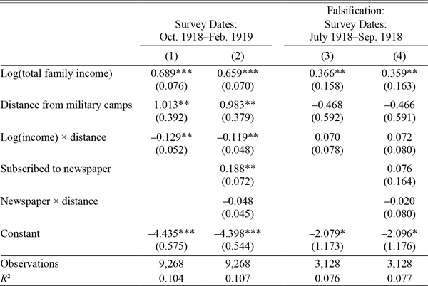
Table 6 presents the results of household-level regressions of a binary indicator for the purchase of a liberty bond within the previous year on household characteristics. Column (1) presents results from using only surveys administered following the fourth liberty loan campaign. The reported estimates indicate that greater log income was associated with a higher probability of liberty bond purchases, and consistent with the IV results presented above, greater distance from the military camps was also associated with a higher probability of a liberty bond purchase. But, in addition, the regression includes an interaction between log income and distance, and the estimated effect is negative: In cities farther away from military camps, the effect of log income on liberty bond subscriptions was smaller. If this is an indication that the more extensive loan campaigns were conducted in regions where the influenza outbreak was less severe, then this could account for the greater magnitude of the IV estimates presented above.
DETERMINANTS OF LIBERTY BOND PURCHASES AMONG BLS SURVEY HOUSEHOLDS, 1918–1919

Notes: This table presents OLS regressions of the effect of household characteristics on a binary measure of liberty bond purchases, from BLS survey data. The dependent variable is equal to 1 if the household purchased a liberty bond within the previous year from the survey date, and its mean value is 0.68. Robust standard errors clustered by city are presented in parentheses. *p < 0.1, **p < 0.05, and ***p < 0.01.
Sources: Authors’ calculations from data in Olney (Reference Olney1995) and U.S. War Department (1920).
Column (2) adds an indicator equal to one if a household subscribed to a newspaper in the past year (as indicated in the survey by some amount spent on newspapers). This is positively associated with liberty bond purchases, indicating that better-informed households were more likely to subscribe. The estimated interaction between newspaper subscriptions and distance reported in the table is negative, a possible indication that the more extensive liberty loan campaigns in the regions where influenza was less severe reached less-informed households. However, this effect is imprecisely estimated.
Finally, Columns (3) and (4) estimate the same regressions using the responses to the survey administered prior to the fourth loan and the influenza outbreak. These likely reflect the effects of the third liberty loan campaign. The results indicate that, as in Columns (1) and (2), household income was an important determinant of liberty bond purchases. However, distance to the military camps was not, and there was no income-distance gradient as with the fourth loan. This is inconsistent with the notion that distance to the camps led to liberty bond subscriptions through some mechanism other than influenza.
THE 1920 ELECTION: RESULTS FROM STATE DATA
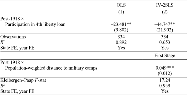
Finally, we investigate whether or not the estimated effects of liberty bonds on election outcomes were decisive, by re-estimating Equation (1) using OLS and 2SLS with state data. Our instrument for liberty bond participation is re-calculated as the population-weighted average distance of all of a state’s counties to the military camps. As we are limited to 48 states, we view this analysis as a simple exercise in which we can assess the plausibility of our estimates and determine whether they could have been decisive. But it also enables us to verify that the effects we found for our sample of counties are not unique to those regions of the country, as the state data include the entire United States.
The results are presented in Table 7. The baseline OLS estimate presented in Column (1) is larger than that obtained from county data, reflecting both the differences in the level of aggregation of the data and the fact that the state data covers a broader geographical area. The 2SLS estimate in Column (2) is again larger than the OLS estimate, but the ratio of the two is roughly similar to that obtained from the county data. As with the county data, the distance measure creates a strong first stage, minimizing any concerns regarding weak instruments.
EFFECT OF LIBERTY LOAN PARTICIPATION ON ELECTORAL OUTCOMES, 1908–1932: STATE DATA

Notes: This table presents OLS and 2SLS regressions using state data. The instrument for liberty loan participation is the mean population-weighted distance of state to military camps. All regressions are weighted by 1920 state population. The fraction of the states’ population in urban areas is included in both the first- and second-stage regressions (not shown). Robust standard errors are clustered by state in parentheses. *p < 0.1, **p < 0.05, and ***p < 0.01.
Sources: Authors’ calculations from data in U.S. Treasury (1918–1921), U.S. War Department (1920), Haines (Reference Haines2010) and Leip (Reference Leip2018).
To determine whether these effects were decisive, we calculate counterfactual Democratic Party vote shares for the 1920 election, assuming that the liberty loan campaigns had never been held and, therefore, that the subscription rates for liberty loans were zero. That is, for each state, we calculate a new Democratic vote share as the old one plus the added share from setting the liberty bond subscription rate to zero, or  $ - {\mathop {\hat \delta}_{2{\rm{SLS}}}} \times libloanpartici{p_i}$.
The 1920 election was a Republican landslide, with electoral vote totals of 404 to 127. Our estimates imply that, in the absence of the liberty bond campaigns, the Democrats would have won 12 additional states and the electoral vote totals would have been 292 (R) to 239 (D).Footnote 23 Thus, this exercise indicates that the effects of liberty bond ownership likely did not tip the balance in the outcome of the election. The Republicans still would have won, only in less of a landslide.
CONCLUSION
This paper has investigated the political effects of the liberty bond drives of WWI. Our analysis indicates that counties that subscribed to the bonds at higher rates turned against the Democratic Party in the 1920 and 1924 presidential elections, relative their voting patterns over the previous decade. The 1920s were a period in which the Republicans dominated American politics, and the effects of liberty bond ownership contributed significantly to that development, although they were unlikely to have been decisive.
This outcome likely reflected voters’ assessments of economic policy outcomes under Democrats and Republicans. Liberty bonds depreciated substantially in late 1919 and in 1920, which came as a shock to many subscribers who had not understood the risks of their investments. This was partly due to McAdoo’s decision to mass market negotiable securities to inexperienced investors and to his successors’ reluctance to allow the Fed to increase interest rates in early 1919, which contributed to the Fed’s decision to increase them quite dramatically when they were finally permitted to do so. Then, subsequent Republican administrations benefitted from the timing of those rate increases, as the Fed finally eased rates in 1921 and 1922, and again in 1924, and liberty bond holders experienced substantial capital gains. This made voters receptive to Republican campaign messages that their leadership promoted prosperity and sound financial management.
Policymakers learned lessons, both positive and negative, from the liberty bonds experience. When the federal debt grew during the Great Depression, then Treasury Secretary Morganthau introduced “baby bonds” (savings bonds)—government securities sold through the nation’s post offices on a continual basis that were, by design, non-negotiable. These bonds protected investors from price fluctuations, and they could be redeemed on demand according to a schedule that incentivized longer holding periods (Garbade 2012). The baby bonds, known formally as Series A, B, C, and D, were described as “a Share in America” (Olney Reference Olney1971), and Morgenthau, like McAdoo before him, believed that their ownership would increase the attachment of ordinary Americans to their nation (Kimble 2006). The safety of Depression-era baby bonds provided the blueprint for the Series E savings bonds used to finance WWII (Morse 1971; Olney Reference Olney1971). The marketing of Series E bonds replicated the liberty loan drives, including the use of short, concentrated campaigns and the mobilization of civil society organizations as a salesforce. To the toolkit inherited from WWI, organizers added the modern medium of radio and hired social scientists to evaluate bond messaging and “segment” the bond-buying public into discrete target audiences (Samuel Reference Samuel1997). But, most importantly, the bonds retained the non-negotiability of Morganthau’s baby bonds, protecting the ordinary households that were induced to support the war effort from subsequent fluctuations in interest rates.
But another important legacy of liberty bonds was the experience of one noteworthy subscriber, Harry Truman. After returning from WWI, Truman had to sell his family’s liberty bonds at severely depreciated prices to raise money, an experience that apparently infuriated him and made him suspicious of the motives behind Fed policy. He, of course, became President in 1945, and at that time, the Fed maintained a wartime policy of actively supporting the prices of government securities by purchasing large quantities of them. After the end of WWII, in response to high inflation, the Fed sought to end this policy but was vigorously opposed by Truman and the Treasury. In 1951, with the Korean War underway and high inflation prevailing, the conflict between the Fed and Truman intensified and Truman took the extraordinary step of asking the entire Federal Open Market Committee to meet with him in the Oval Office. In that meeting, Truman stated that he did not want “the people who hold our bonds now to have done to them what was done to him.”Footnote 24 The conflict escalated further and was ultimately resolved through the negotiation of the Treasury-Fed Accord, which helped establish the foundations of the Fed’s modern independence. In more ways than one, liberty bonds shaped the evolution of American monetary and fiscal institutions.