2 Preliminaries

A non-empty set X with an operator $R\colon X \times X \to X \times X$ , mapping $(x,y) \mapsto (R_1(x,y), R_2(x,y) )$ , is called a biquandle if the following holds:

1. (1) R satisfies the Yang–Baxter relation, that is,

   (2.1) $$ \begin{align} (R \times \mathrm{id}) (\mathrm{id} \times R) (R \times \mathrm{id})=(\mathrm{id} \times R) (R \times \mathrm{id}) (\mathrm{id} \times R), \end{align} $$

   where $\mathrm {id}$ is the identity map on X;

2. (2) R is invertible;

3. (3) $R_1$ is left-invertible, meaning that for any $x,z \in X$ , there exists a unique $y \in X$ such that $R_1(x,y)=z$ ;

4. (4) $R_2$ is right-invertible, meaning that for any $y, w \in X$ , there exists a unique $x \in X$ such that $R_2(x,y)=w$ ;

5. (5) R satisfies the type I condition, which is, for any $a \in X$ , there exists a unique $x \in X$ such that $R(x,a)=(x,a)$ .

Note that the type I condition is equivalent to the following: for given $a \in X$ , there exists a unique $y \in X$ such that $R(a, y)=(a,y)$ .

The following are some examples.

We revisit the definition of virtual biquandles from [Reference Kauffman and Manturov23]. A virtual biquandle is a triplet $(X,f,R)$ , where $(X,R)$ is a biquandle and $f: X \to X$ is an automorphism of $(X,R)$ .

The following are straightforward examples of virtual biquandles.

A homomorphism from $(X,f,R)$ to $(Y,f',R')$ is a map $\phi : (X,f,R) \to (Y,f', R')$ such that $\phi :(X,R) \to (Y, R')$ is a biquandle homomorphism and $\phi \circ f= f' \circ \phi $ .

The proof of Proposition 2.5 can be found in [Reference Elhamdadi and Singh10]; however, for the sake of completeness, we recall it here.

Proof The invertibility of R and f gives the invertibilty of $VR$ as

$$\begin{align*}VR= (\mathrm{id} \times f^{-1})~R~(\mathrm{id} \times f).\end{align*}$$

Thus it is sufficient to prove that $VR$ is a Yang–Baxter operator.

L.H.S of Equation (2.1) is

$$ \begin{align*} &(VR \times \mathrm{id} ) (\mathrm{id} \times VR) (VR \times \mathrm{id})~~(x,y,z)\\&=(VR \times \mathrm{id}) (\mathrm{id} \times VR)~~ \big( R_1(x,f(y)), R_2(f^{-1}(x),y), z \big)\\ &=(VR \times \mathrm{id} ) ~~ \big( R_1(x,f(y)), R_1( R_2 (f^{-1}(x), y), f(z) ), R_2 ( R_2 (f^{-2}(x), f^{-1}(y)), z) \big)\\ &=\big( R_1 \big( R_1(x,f(y)), R_1(R_2(x,f(y)), f^2(z) ) \big),\\&R_2 \big( R_1 (f^{-1}(x), y), R_1 (R_2(f^{-1}(x),y), f(z))\big), R_2 ( R_2 (f^{-2}(x), f^{-1}(y)), z) \big). \end{align*} $$

R.H.S of Equation (2.1) is

$$ \begin{align*} &(\mathrm{id} \times VR) (VR \times \mathrm{id}) (\mathrm{id} \times VR)~~(x,y,z)\\&=(\mathrm{id} \times VR) (VR \times \mathrm{id}) ~~\big( x, R_1(y,f(z)), R_2 (f^{-1}(y),z) \big)\\ &=(\mathrm{id} \times VR) ~~\big( R_1\big( x, R_1(f(y), f^2(z)), R_2(f^{-1}(x), R_1(y, f(z))), R_2(f^{-1}(y),z) \big) \big)\\ &= \big( R_1(x, R_1(f(y), f^2(z))), R_1(R_2(f^{-1}(x), R_1(y, f(z)))), R_2(y, f(z)) ,\\ &R_2(R_2(f^{-2}(x), R_1(f^{-1}(y),z)), R_2(f^{-1}(y),z)) \big). \end{align*} $$

Now L.H.S=R.H.S, if and only if the following equations hold for all $x,y,z \in X$ :

(2.2) $$ \begin{align} &R_1 \big( R_1(x,f(y)), R_1(R_2(x,f(y)), f^2(z) ) \big)= R_1\big(x, R_1(f(y), f^2(z))\big) \end{align} $$

(2.3) $$ \begin{align} &R_2 \big( R_1 (f^{-1}(x), y), R_1 (R_2(f^{-1}(x),y), f(z))\big) \nonumber\\ &=R_1\big(R_2(f^{-1}(x), R_1(y, f(z))), R_2(y,f(z))\big) \end{align} $$

(2.4) $$ \begin{align} &R_2 \big( R_2 (f^{-2}(x), f^{-1}(y)), z\big) =R_2\big(R_2(f^{-2}(x), R_1(f^{-1}(y),z)), R_2(f^{-1}(y),z)\big). \end{align} $$

Equations (2.2), (2.3), and (2.4) follow from that

$$\begin{align*}(R \times \mathrm{id}) (\mathrm{id} \times R) (R \times \mathrm{id})(x, f(y), f^2(z))=(\mathrm{id} \times R)(R \times \mathrm{id}) (\mathrm{id} \times R)(x,f(y), f^2(z)) \end{align*}$$

as R is a Yang–Baxter operator.

The construction of a biquandle from a virtual biquandle, in Proposition 2.5, gives a functor from the category of virtual biquandles to the category of biquandles. This follows from the observation that if we have a morphism $g: (X,f, R) \to (X',f',R')$ in the virtual biquandle category, then we have the following commutative diagrams,

implying the following commutative diagram

From the above discussion, we note down the following result.

From Proposition 2.6 it follows that $(X,f, VR)$ is a virtual biquandle.

We recall the following notions of virtual knot theory from [Reference Kauffman21].

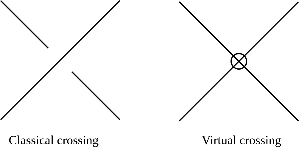
A virtual link diagram is a generic immersion of a finitely many circles into the Euclidean plane $\mathbb {R}^2$ or the $2$ -sphere $\mathbb {S}^2$ , where the double points are decorated either as classical crossings or virtual crossings, as shown in Figure 1.

Figure 1

Classical crossing and virtual crossing.

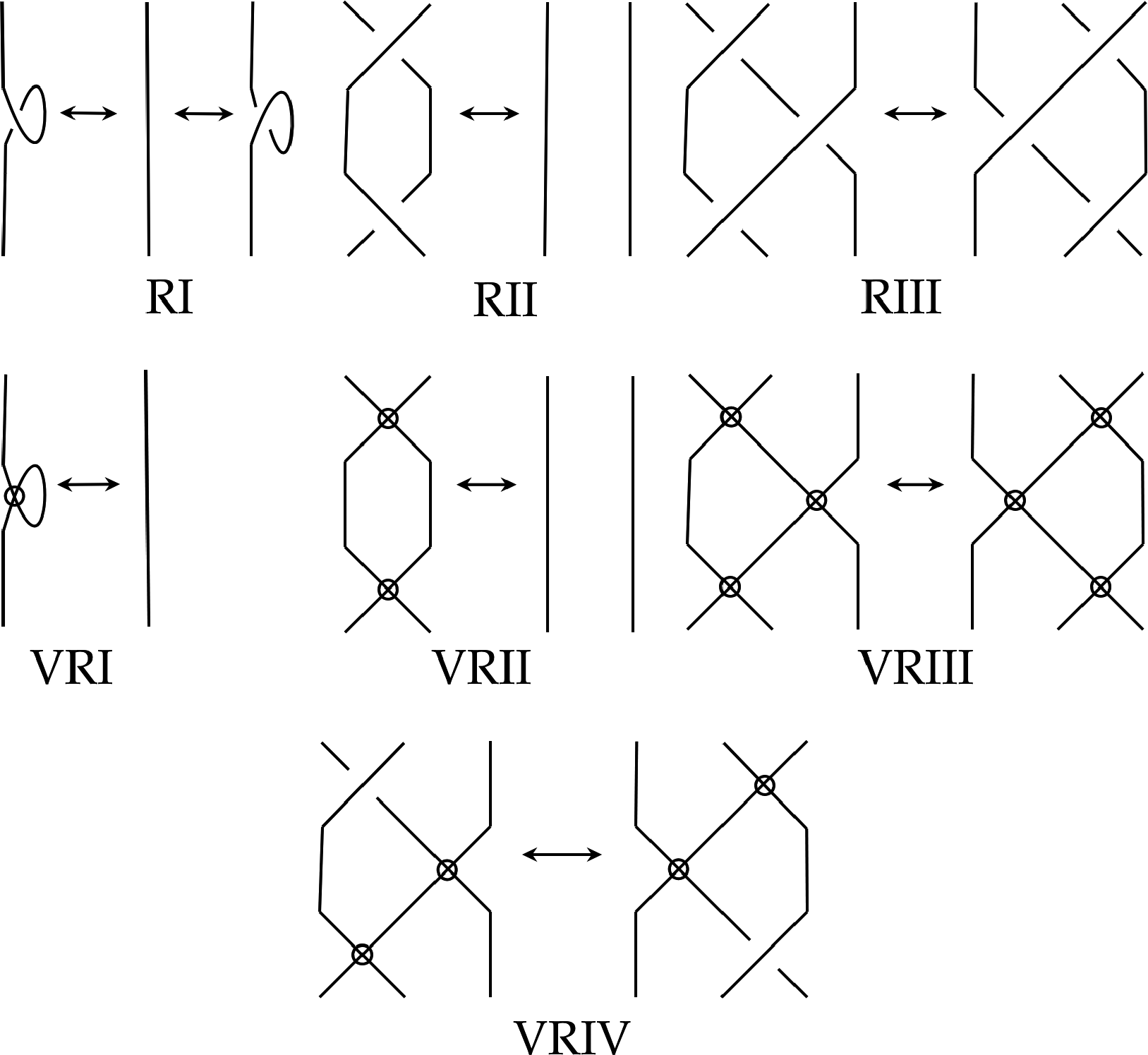
Two virtual link diagrams are said to be equivalent if they are related by a finite sequence of planar isotopies and generalized Reidemeister moves shown in Figure 2. A virtual link is an equivalence class of virtual link diagrams under the generalized Reidemeister moves and planar isotopies.

Figure 2

Generalized Reidemeister moves.

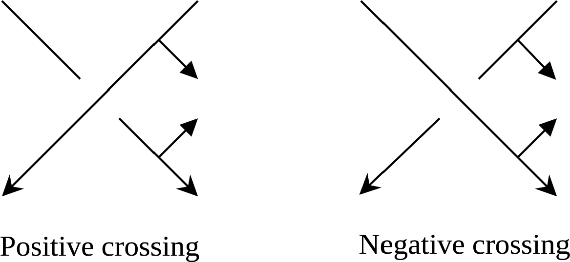
In an oriented virtual link diagram, a classical crossing is positive if the co-orientation of the over-arc and that of the under-arc match with the orientation of the plane, otherwise it is negative. Positive and negative crossings are depicted in Figure 3.

Figure 3

Positive and negative crossings.

Figure 4

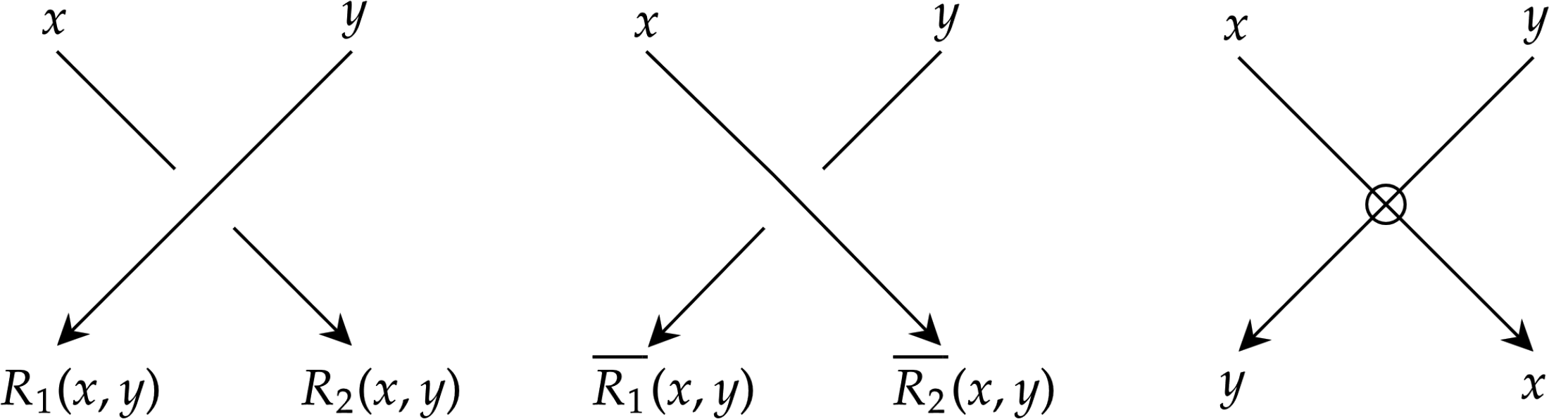
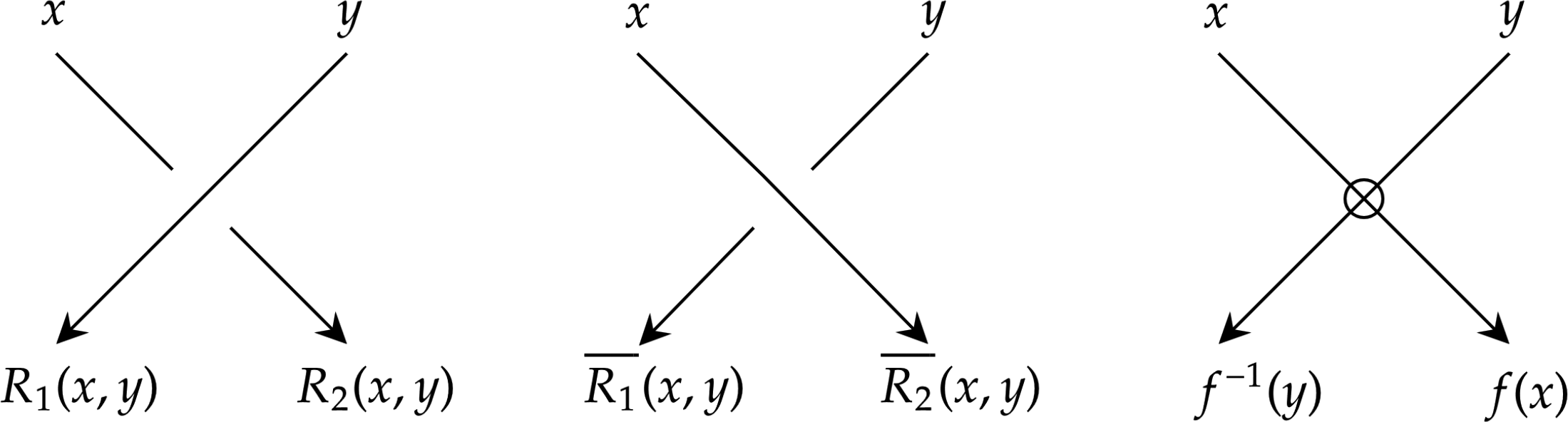
Labeling rules for biquandle.

Figure 5

Labeling rules for virtual biquandle.

Consider an oriented virtual link L, represented by a virtual link diagram D. In D, a semiarc is defined as an arc between two consecutive double points. The associated fundamental biquandle $BQ(L)$ is the quotient of the free biquandle generated by the labels on the set of semiarcs in D. This is done by applying the equivalence relation induced by the relations at crossing in D, as shown in Figure 4. This association is independent of the diagrams used to represent L. For more details, we refer the readers to [Reference Kauffman and Manturov23, Section 2.6] and [Reference Fenn, Jordan-Santana and Kauffman12, Reference Hrencecin and Kauffman14].

In a similar way, one can associate a fundamental virtual biquandle ( $VBQ(L), f , R)$ to L. This virtual biquandle is defined as the quotient of the free virtual biquandle generated by the labels on the set of semiarcs in the virtual link diagram D. This is done by applying the equivalence relation induced by the relations at the crossings in D, as shown in Figure 5. Importantly, the virtual biquandle ( $VBQ(L), f, R)$ is independent of the diagram D up to isomorphisms. See [Reference Kauffman and Manturov23, Section 2.6] for more details.

A coloring of a virtual link L by a virtual biquandle $(X,f',R')$ is a virtual biquandle homomorphism $\phi :(\hspace{-1pt}VBQ(L), f, R) \to (X,f',R')$ . Note that labeling the semiarcs of the diagram D with elements from $(X,f',R')$ , following the rules depicted in Figure 5, results in a coloring of L.

3 Set theoretic bijection between the set of colorings by biquandles and virtual biquandles

In this section, we prove that if L is a virtual link, then the set of colorings of L by a virtual biquandle $(X,f,R)$ under the rules illustrated in Figure 5 is in bijection with the set of colorings of L by $(X,VR)$ under the rules illustrated in Figure 4.

First recall the definition of the virtual braid group $VB_n$ on n-strands, which has the following presentation (see [Reference Bardakov and Bellingeri1, Theorem 4]):

• • Generators: $\sigma _1, \sigma _2, \ldots , \sigma _{n-1},\rho _1, \rho _2, \ldots , \rho _{n-1}.$

• • Relations:

  $$ \begin{align*} &\sigma_i \sigma_{i+1} \sigma_i = \sigma_{i+1} \sigma_i \sigma_{i+1}, ~i=1,2,\ldots, n-2;\\ &\sigma_i \sigma_j = \sigma_j \sigma_i, ~|i-j| \geq 2;\\ &\rho_i\rho_{i+1} \rho_i = \rho_{i+1}\rho_i \rho_{i+1}, ~ i=1,2,\ldots,n-2;\\ &\rho_i \rho_j =\rho_j \rho_i,~ | i-j| \geq 2;\\ &\rho_i^2 =1,~ i=1,2,\ldots,n-1;\\ &\sigma_i \rho_j = \rho_j \sigma_i,~ |i-j| \geq 2;\\ &\rho_i \rho_{i+1} \sigma_i = \sigma_{i+1} \rho_i \rho_{i+1},~ i=1,2,\ldots, n-2. \end{align*} $$

Geometrically, $\sigma _i$ , $\sigma _i^{-1}$ and $\rho _i$ are shown in Figure 6.

Figure 6

Generators of virtual braid group $VB_n$ .

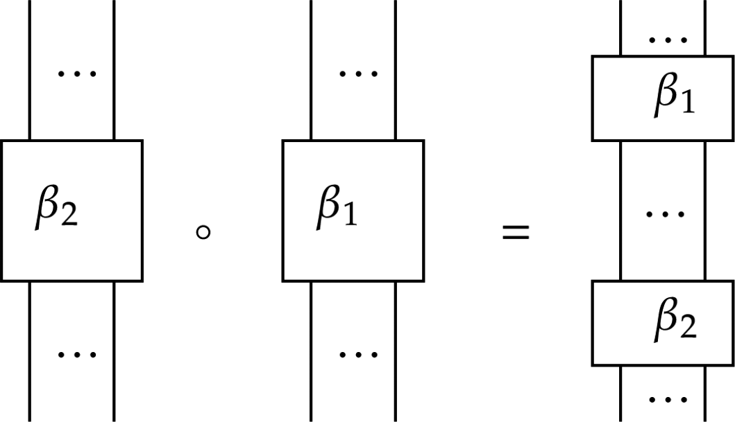
For $\beta _1, \beta _2 \in VB_n$ , the composition $\beta _2 \beta _1$ in $VB_n$ represents the braid shown in Figure 7.

Figure 7

Composition operation on $VB_n$ .

Let $VB_n$ be the virtual braid group on n-strands and $(X, f, R)$ be a virtual biquandle. Then $VB_n$ acts on the product $X^n$ of n copies of X by the representation

$$\begin{align*}\phi: VB_n \to \operatorname{Aut}(X^n) \end{align*}$$

defined as follows:

$$ \begin{align*} &\phi(\sigma_i) : \left\{\!\!\! \begin{array}{l} x_i \mapsto R_1(x_i,x_{i+1}), \\ x_{i+1} \mapsto R_2(x_i,x_{i+1}), \\ x_j \mapsto x_j, \textrm{ for } j \neq i, i+1, \\ \end{array} \right.~~~ &\phi(\rho_i) : \left\{\!\!\! \begin{array}{l} x_i \mapsto f^{-1}(x_{i+1}), \\ x_{i+1} \mapsto f(x_i), \\ \end{array} \right. \end{align*} $$

for $1 \leq i \leq n-1$ . It is easy to check that

Now, consider an automorphism

$$\begin{align*}\theta: X^n \to X^n\end{align*}$$

defined as

$$\begin{align*}\theta = f^{n-1} \times f^{n-2} \times \cdots \times f^{n-i} \times \cdots \times f \times \mathrm{id}.\end{align*}$$

Note that

$$\begin{align*}\theta^{-1} = f^{-n+1} \times f^{-n+2} \times \cdots \times f^{-n+i} \times \cdots \times f^{-1} \times \mathrm{id}.\end{align*}$$

Now define a new action

$$\begin{align*}\psi: VB_n \to \operatorname{Aut}(X^n)\end{align*}$$

of $VB_n$ on $X^n$ given by

$$\begin{align*}\psi(\beta)= \theta \circ \phi (\beta) \circ \theta^{-1}.\end{align*}$$

We give the following explicit images of the generators of $VB_n$ under the representation $\psi $ :

$$ \begin{align*} &\psi(\sigma_i) : \left\{ \begin{array}{l} x_i \mapsto R_1\big(x_i,f(x_{i+1})\big), \\ x_{i+1} \mapsto R_2\big(f^{-1}(x_i),x_{i+1}\big), \\ x_j \mapsto x_j, \textrm{ for } j \neq i, i+1, \\ \end{array} \right.~~~ &\psi(\rho_i) : \left\{ \begin{array}{l} x_i \mapsto x_{i+1}, \\ x_{i+1} \mapsto x_i \\ \end{array} \right. \end{align*} $$

and

By [Reference Kamada19], for every virtual link L there exists a virtual braid $\beta $ whose closure is L.

As a result of Theorem 3.2, we have the following corollary.

Thus, the number of colorings of a virtual link L by a virtual biquandle can be retrieved from colorings of L by a suitable biquandle.

4 Deriving Fundamental Virtual Biquandle from Classical Crossings

Let $(FVBQ_n,f,R)$ denotes the free virtual biquandle on the set $\{x_1, x_2, \ldots , x_n\}$ . The virtual braid group $VB_n$ on n-strands acts on $FVBQ_n$ via the representation

$$\begin{align*}\Phi: VB_n \to \operatorname{Aut}\big((FVBQ_n, f, R)\big)\end{align*}$$

defined as follows:

$$ \begin{align*} &\Phi(\sigma_i) : \left\{ \begin{array}{l} x_i \mapsto R_1(x_i,x_{i+1}), \\ x_{i+1} \mapsto R_2(x_i,x_{i+1}), \\ x_j \mapsto x_j, \textrm{ for } j \neq i, i+1, \\ \end{array} \right.~~~ &\Phi(\rho_i) : \left\{ \begin{array}{l} x_i \mapsto f^{-1}(x_{i+1}), \\ x_{i+1} \mapsto f(x_i). \\ \end{array} \right. \end{align*} $$

Note that for $1 \leq i \leq n-1$ ,

$$ \begin{align*} \Phi(\sigma_{i}) \circ f &= f \circ \Phi(\sigma_{i})\\ \Phi(\rho_{i}) \circ f&=f \circ \Phi(\rho_{i}).\\ \end{align*} $$

One can check that

Now, consider an automorphism

$$\begin{align*}\Theta: (FVBQ_n, f, R) \to (FVBQ_n, f, R)\end{align*}$$

defined as

$$\begin{align*}\Theta(x_i)=f^{n-i}(x_i).\end{align*}$$

Now define a new action of $VB_n$ on $(FVBQ_n, f,R)$

$$\begin{align*}\Psi: VB_n \to \operatorname{Aut}((FVBQ_n, f,R))\end{align*}$$

given by

$$\begin{align*}\Psi(\beta)= \Theta \circ \Phi (\beta) \circ \Theta^{-1}.\end{align*}$$

We write down the images of the generators of $VB_n$ under the map $\Psi $ :

$$ \begin{align*} &\Psi(\sigma_i) : \left\{ \begin{array}{l} x_i \mapsto R_1\big(x_i,f(x_{i+1})\big), \\ x_{i+1} \mapsto R_2\big(f^{-1}(x_i),x_{i+1}\big), \\ x_j \mapsto x_j, \textrm{ for } j \neq i, i+1, \\ \end{array} \right.~~~ &\Psi(\rho_i) : \left\{ \begin{array}{l} x_i \mapsto x_{i+1}, \\ x_{i+1} \mapsto x_i \\ \end{array} \right. \end{align*} $$

and

For a given $\beta \in VB_n$ , associate a virtual biquandle $VBQ(\Phi ,\beta ) = FVBQ_n/\mathcal {R}$ , where $\mathcal {R}$ is the equivalence relation generated by the set $\{ \Phi (\beta )(x_i)=x_i~|~ 1 \leq i \leq n\}$ . We write $VBQ(\Phi ,\beta )$ in a presentation form as follows:

$$\begin{align*}\langle x_1, \ldots, x_n, f, R~|~\Phi(\beta)(x_i)=x_i\rangle. \end{align*}$$

Similarly, replacing the representation $\Phi $ with $\Psi $ , we associate a virtual biquandle $VBQ(\Psi , \beta )= FVBQ_n/\mathcal {R'}$ , where $\mathcal {R'}$ is the equivalence relation generated by the set $\{\Psi (\beta )(x_i)=x_i~|~ 1 \leq i \leq n \}$ . A presentation form of $VBQ(\Psi , \beta )$ is as follows:

$$\begin{align*}\langle x_1, \ldots, x_n, f, R~|~\Psi(\beta)(x_i)=x_i\rangle. \end{align*}$$

In [Reference Kauffman and Manturov23, Section 2.6], the formal virtual biquandle notion is defined. The term “formal” refers to a framework for defining various notions of virtual quandles based on the coloring rules at virtual crossings. For any such model, the corresponding algebraic structure and its presentation can be determined by defining a specific representation of virtual braids into the automorphism group of some algebra. For instance, presentations of biquandles associated with virtual knots have been studied through braid representations in [Reference Hrencecin and Kauffman14, Section 5]. This technique is well-known in mathematical folklore, and we refer the reader to [Reference Wada27, Section 1] for a proof in a specific setting, though the overall idea remains the same in different scenarios. In our case, the notion of the associated fundamental virtual biquandle corresponds to the representation $\Phi : VB_n \to \operatorname {Aut}(FVBQ_n, f, R)$ of virtual braids. Consequently, we obtain the following result.

Consequently, the following result follows.

Thus, the associated virtual biquandle $VBQ(\Phi ,\beta )$ is an invariant of virtual links.

Proof For $\beta \in VB_n$ , the virtual biquandle $VBQ(\Phi ,\beta )$ has a following presentation

$$\begin{align*}\langle x_1, \ldots, x_n, f,R~|~\Phi(\beta)(x_i)=x_i \textrm{ for } 1 \leq i \leq n \rangle. \end{align*}$$

Consider the automorphism $\Theta : FVBQ_n \to FVBQ_n$ as defined above. Since $\Theta $ is an automorphism, thus

$$ \begin{align*} VBQ(\Phi,\beta)\cong &\langle x_1, \ldots, x_n,f, R~|~\Theta(\Phi(\beta)(x_i))=\Theta(x_i) \textrm{ for } 1 \leq i \leq n \rangle\\ \cong & \langle x_1, \ldots, x_n,f, R~|~\Theta\circ\Phi(\beta)\circ\Theta^{-1}(\Theta(x_i))=\Theta(x_i) \textrm{ for } 1 \leq i \leq n \rangle\\ \cong & \langle x_1, \ldots, x_n,f, R~|~\Psi(\beta)(\Theta(x_i))=\Theta(x_i) \textrm{ for } 1 \leq i \leq n \rangle\\ \cong & \langle x_1, \ldots, x_n,f, R~|~\Psi(\beta)(f^{n-i}(x_i))=f^{n-i}(x_i) \textrm{ for } 1 \leq i \leq n \rangle\\ \cong & \langle x_1, \ldots, x_n,f, R~|~\Psi(\beta)(x_i)=x_i \textrm{ for } 1 \leq i \leq n \rangle\\ \cong &VBQ(\Psi, \beta). \end{align*} $$

This concludes the proof.

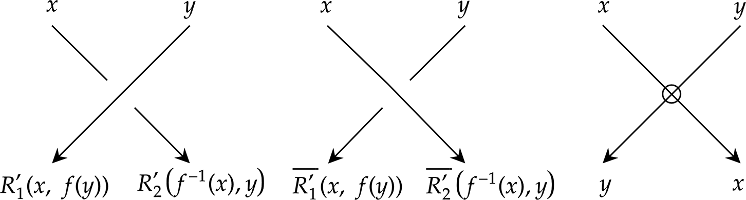
Let L be an oriented virtual link represented by a virtual link diagram D. Then we associate a virtual biquandle $(X, f', R')$ to L defined as the quotient of a free virtual biquandle, which is generated by the labels on the set of semiarcs in the diagram D, by the equivalence relation induced by the relations at the crossings in D as shown in Figure 8.

Theorem 4.4 The virtual biquandle $(X,f',R')$ is isomorphic to the fundamental virtual biquandle $(VBQ(L), f, R)$ .

Figure 8

New labeling rules.

Hence, the fundamental virtual biquandle can be retrieved from just classical crossings in a virtual link.

Figure 9

Depiction of new labeling rules on Gauss diagrams.

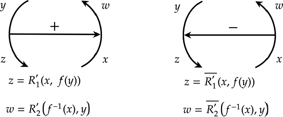
A Gauss diagram consists of a finite number of circles oriented anticlockwise with a finite number of signed arrows whose heads and tails lie on the circles. For every oriented virtual link diagram L one can construct a Gauss diagram, where the arrows corresponds to the classical crossings in L. Figure 9 depicts the encoding of new labeling rules (from Figure 8) on Gauss diagrams. Thus, we can recover the fundamental virtual biquandle for a given virtual link L directly from a Gauss diagram representing L.

5 Concluding remarks

In this article, using virtual braid group representations, we prove that the coloring number invariant of virtual links, derived from virtual biquandles, can be obtained from colorings by biquandles. Also, by Remark 2.7, we note that colorings using biquandles can be recovered from those using virtual biquandles. Moreover, Theorem 4.4 suggests that any invariant stemming from the fundamental virtual biquandle can be extracted solely from classical crossings in virtual link diagrams. This suggests that classical crossings in virtual links may encompass more information than previously acknowledged. In our ongoing work [Reference Elhamdadi and Singh10], we are integrating the unary operator of virtual biquandles with Alexander numbering of links and standard biquandle coloring, thereby enhancing the state-sum invariant. In our forthcoming research, we aim to delve further into the “virtualized” invariants, such as the Alexander polynomial as defined in [Reference Boden and Chrisman4, Reference Jaeger, Kauffman and Saleur15, Reference Silver and Williams26], and the state-sum invariant derived from virtual biquandles [Reference Ceniceros and Nelson8, Reference Farinati and García Galofre11], shedding further light on their intricacies.